Stochastic Implied Trees: Arbitrage Pricing With Stochastic Term and Strike Structure of Volatility

Technical Notes

Stochastic Implied Trees:

Arbitrage Pricing With

Stochastic Term and Strike

Structure of Volatility

Emanuel Derman

Iraj Kani

Copyright 1997 Goldman, Sachs & Co. All rights reserved.

This material is for your private information, and we are not soliciting any action based upon it. This report is not to be construed as an offer to sell or the solicitation of an offer to buy any security in any jurisdiction where such an offer or solicitation would be illegal. Certain transactions, including those involving futures, options and high yield securities, give rise to substantial risk and are not suitable for all investors. Opinions expressed are our present opinions only. The material is based upon information that we consider reliable, but we do not represent that it is accurate or complete, and it should not be relied upon as such. We, our affiliates, or persons involved in the preparation or issuance of this material, may from time to time have long or short positions and buy or sell securities, futures or options identical with or related to those mentioned herein.

This material has been issued by Goldman, Sachs & Co. and/or one of its affiliates and has been approved by Goldman Sachs International, regulated by The Securities and Futures Authority, in connection with its distribution in the United Kingdom and by Goldman Sachs Canada in connection with its distribution in Canada. This material is distributed in Hong Kong by Goldman Sachs (Asia) L.L.C., and in Japan by Goldman Sachs (Japan) Ltd. This material is not for distribution to private customers, as defined by the rules of The Securities and Futures Authority in the United Kingdom, and any investments including any convertible bonds or derivatives mentioned in this material will not be made available by us to any such private customer. Neither Goldman, Sachs & Co. nor its representative in Seoul, Korea is licensed to engage in securities business in the Republic of Korea. Goldman Sachs International or its affiliates may have acted upon or used this research prior to or immediately following its publication. Foreign currency denominated securities are subject to fluctuations in exchange rates that could have an adverse effect on the value or price of or income derived from the investment. Further information on any of the securities mentioned in this material may be obtained upon request and for this purpose persons in Italy should contact Goldman Sachs S.I.M. S.p.A. in Milan, or at its London branch office at 133 Fleet Street, and persons in Hong Kong should contact Goldman Sachs Asia L.L.C. at 3 Garden Road. Unless governing law permits otherwise, you must contact a Goldman Sachs entity in your home jurisdiction if you want to use our services in effecting a transaction in the securities mentioned in this material.

SUMMARY

In this paper we present an arbitrage pricing framework for valuing and hedging contingent equity index claims in the presence of a chastic term and strike structure of volatility. Our approach to sto-chastic volatility is similar to the Heath-Jarrow-Morton (HJM) approach to stochastic interest rates. Starting from an initial set of index options prices and their associated local volatility surface, we show how to construct a family of continuous time stochastic processes which define the arbitrage-free evolution of this local volatility surface through time. The no-arbitrage conditions are similar to, but more involved than, the HJM conditions for arbitrage-free stochastic move-ments of the interest rate curve. They guarantee that even under a general stochastic volatility evolution the initial options prices, or their equivalent Black-Scholes implied volatilities, remain fair.

We introduce stochastic implied trees as discrete implementations of our family of continuous time models. The nodes of a stochastic implied tree remain fixed as time passes. During each discrete time step the index moves randomly from its initial node to some node at the next time level, while the local transition probabilities between the nodes also vary. The change in transition probabilities corresponds to a general (multifactor) stochastic variation of the local volatility surface. Starting from any node, the future movements of the index and the local volatilities must be restricted so that the transition prob-abilities to all future nodes are simultaneously martingales. This guarantees that initial options prices remain fair. On the tree, these martingale conditions are effected through appropriate choices of the drift parameters for the transition probabilities at every future node, in such a way that the subsequent evolution of the index and of the local volatility surface do not lead to riskless arbitrage opportunities among different option and forward contracts or their underlying index.

You can use stochastic implied trees to value complex index options, or other derivative securities with payoffs that depend on index volatil-ity, even when the volatility surface is both skewed and stochastic. The resulting security prices are consistent with the current market prices of all standard index options and forwards, and with the absence of future arbitrage opportunities in the framework. The calcu-lated options values are independent of investor preferences and the market price of index or volatility risk. Stochastic implied trees can also be used to calculate hedge ratios for any contingent index security in terms of its underlying index and all standard options defined on that index.

________________________

TABLE OF CONTENTS

INTRODUCTION... 1

LOCALVOLATILITYSURFACE: THEEFFECTIVETHEORY OFVOLATILITY... 4

THEEFFECTIVEINTERESTRATETHEORY ... 5

THEEFFECTIVEVOLATILITYTHEORY... 8

TOWARDS ASTOCHASTICTHEORY OFVOLATILITY ... 11

The Stochastic Interest Rate Theory ... 11

The Stochastic Volatility Theory ... 12

The HJM Conditions and the Stochastic Theory of Interest Rates... 14

The NO-ARBITRAGECONDITIONS AND THESTOCHASTICTHEORY OFVOLATILITY.. 16

STOCHASTICIMPLIEDTREES... 21

Our Notation in Discrete Time ... 24

A Simple Example ... 27

Pricing of Some Contracts with Payoffs Based on Realized Volatility ... 35

HEDGINGINDEX ANDVOLATILITYRISKS INSTOCHASTICVOLATILITYMODELS... 36

MOREREALISTICSTOCHASTICVOLATILITYMODELS... 37

SUMMARY... 38

APPENDIX A: EXPECTATIONDEFINITIONS OFLOCALVOLATILITY ... 39

APPENDIX B: MATHEMATICS OFEFFECTIVETHEORIES ... 43

APPENDIX C: LOCALVOLATILITYVARIATIONALFORMULAS INEFFECTIVE VOLATILITYTHEORIES ... 45

APPENDIX D: THENO-ARBITRAGECONDITIONS AND THEEXISTENCE OF THE EQUIVALENTMARTINGALEMEASURE INSTOCHASTICVOLATILITYTHEORIES... 48

The Black-Scholes theory of options pricing [Black 1973] assumes that stock prices are stochastic and vary lognormally, but that future stock volatilities, interest rates and dividend yields are known and determinis-tic. The theory is based on the exclusion of arbitrage: an option’s payoff can be replicated by that of a time-varying portfolio of stock and riskless bonds, and must therefore at any time have the same value as the portfo-lio. The most compelling consequence of this arbitrage-free approach is that options values are preference-free: investors of all risk preferences can agree on the unique fair value of an option. This transcendent qual-ity of the theory has led to its great practical success, spawning more than two decades of intensive research that extended it to other underly-ers and relaxed its basic assumptions so as to better match the observed behavior of options markets and underlyers. The current generation of models, even though they treat underlyers more realistically and can be calibrated to prevailing options market prices, are still based on an arbi-trage-free approach, admitting no arbitrage opportunities in their theo-retical framework.

The history of interest rate options pricing illustrates this development. Original models were simple adaptations the Black-Scholes formula with bonds, rather than stocks, as the underlyers. Today, most interest rate options pricing models assume interest rates themselves are stochastic and mean-reverting, allow for several stochastic factors, and can be cali-brated to observed initial bond prices (and their volatilities), while con-straining future interest-rate evolution to be arbitrage-free. These models fall into two basic families. Equilibrium models1 consider inter-est rate processes depending on one or more state variables and are derived from general equilibrium arguments. The market prices of risk are then derived from associated characteristics of the yield curve (such as level, slope, curvature, etc.) or bond prices. In general these models are not calibrated to all current bond prices, and may therefore contain initial arbitrage violations. Arbitrage-free models, in contrast, are cali-brated to all initial bond prices and also admit no future arbitrage viola-tions. They achieve this in two different ways. The first class2 use stochastic interest rate processes that automatically generate arbitrage-free future scenarios, and equip the process with enough parameters to be forcibly calibrated to the initial traded bond prices. The second class3, instead, start with exogenously specified stochastic process for bond prices or forward rates. They then derive constraints on the evolution of bond prices or forward rates so that no future arbitrages occur.

1. See, for example, Cox, Ingersoll and Ross [1985].

The history of stochastic volatility modeling is shorter but still similar to the history of stochastic interest rates. Existing stochastic volatility models fall into two basic families. Complete-market models4specify con-ditions under which the financial market is complete in the presence of the volatility risk. They posit (if necessary) hypothetical traded volatility instruments that can be used to hedge the volatility risk and complete the market. Contingent claim prices in these models depend critically on the price dynamics of the volatility instruments and may also implicitly depend on the market price(s) of volatility risk. Equilibrium models5 tend to assume (rather than derive) some parametric form for the sto-chastic evolution of the index and its volatility in equilibrium, and then derive implicit options valuation formulas which depend on the parame-ters of the process. The traded options prices are then inverted for the unknown parameters.

Complete-market models can be somewhat arbitrary and sometimes unnatural because of the specific assumptions they make about the hypothetical volatility instruments. The equilibrium volatility models have the drawback that the choice of the parametric form for the under-lying stochastic processes remains largely arbitrary. In addition, it is usually difficult to invert complex and non-linear options prices to obtain the parameters. Finally, ad hoc specification of the market prices of risk can lead to violations of arbitrage6.

In this paper we propose a new arbitrage-based approach to contingent claims valuation with stochastic volatility7, similar to the Heath-Jarrow-Morton (HJM) methodology for stochastic interest rates8. We begin with a continuous time economy with multiple factors. We work with local (forward) volatilities, instead of implied volatilities (or option prices), imposing an exogenous stochastic structure on the local volatility sur-face. The primacy of the local volatility surface in our work is analogous to that of the forward rate curve in the HJM framework. Our model takes as given the initial local volatility surface and posits a general multi-factor continuous time stochastic process for its evolution across time. To ensure that this process is consistent with an arbitrage-free economy we characterize the conditions which guarantee absence of

4. See, for example, Merton [1973], Cox and Ross [1976], Johnson and Shanno [1987], Eisenberg and Jarrow [1994].

5. See, for example, Wiggins [1977], Hull and White [1977], Stein and Stein [1991]. 6. See Cox, Ingersoll and Ross [1985], Heath, Jarrow and Morton [1992].

7. Presented in Risk Advanced Mathematics for Derivatives Conference, New York,

December 1997.

explicit arbitrage opportunities (at any future time) among the various option (and futures) contracts defined and traded on the underlying index. Under these conditions markets are complete and contingent claim valua-tion is preference-free. Unfortunately, in contrast to the HJM condivalua-tions, here the arbitrage-free conditions are complex and non-linear (integral) equations, which are difficult to use in their continuous form.

We then introduce Stochastic Implied Trees as a discrete-time framework where the volatility surface undergoes multi-factor (arbitrage-free) sto-chastic variations. Here we work with trinomial stosto-chastic implied trees9. The location of the nodes in this kind of tree are fixed but the transition probabilities vary stochastically as time changes and index level moves. As time evolves, the index level moves randomly from node to node while local volatilities (and concurrently the transition probabilities) fluctuate sto-chastically across the tree. Starting from any initial node, the future move-ments of the index and the local volatility surface must be restricted so that total transition probabilities to all future nodes are simultaneously martingales. On the tree, these martingale conditions can be satisfied by making an appropriate choice of the drift parameter for every future node. In the discrete time framework defined by the stochastic implied tree, this process step-by-step guarantees absence of arbitrage opportunities among different option (and forward) contracts and the underlying index.

We draw extensively on the analogy between interest rates and volatility throughout this paper. We begin by reviewing the concept of the local (for-ward) volatility surface and the effective theory of volatility which it defines. The local volatility surface is the options world analogue of the for-ward interest rate curve. Standard option prices calculated using today’s local volatility surface match their market prices, just as the bond prices calculated from today’s forward rate curve match their market prices. The dynamics of standard option prices, as defined by today’s local volatility surface, albeit arbitrage-free, is based on the assumption of non-stochastic volatility, as portrayed by the static (non-random) nature of the local vola-tility surface. This effective dynamics of option prices is analogous to the deterministic, but arbitrage-free, bond price dynamics which result from a static forward rate curve. To allow stochastic dynamics we introduce exog-enous stochastic structure on the effective theory. This is to say that we allow general (multi-factor) fluctuations of the local volatility surface as time and spot index level change. We impose dynamical conditions which explicitly guarantee absence of arbitrage among standard options, for-wards and the underlying index. This process will augment an effective theory of volatility to a full stochastic theory of volatility in a manner which is the hallmark of the HJM approach to stochastic interest rates.

We can think of local volatility

σ

esti-mate of instantaneous volatility at the future market level K and future time T. Local volatilities corresponding to different future market levels and times together comprise the local volatility surface. The local volatility surface indicates the fair value of future index volatility at future market levels and times as implied by the spec-trum of available standard option (and forward contract) prices.

The relationship between the local volatilities and option prices (or implied volatilities) in the options world is analogous to the relation-ship between the forward rates and bond prices (or yield-to-maturi-ties) in the fixed income world. We can calculate the forward interest rates fT corresponding to the future times T from the spectrum of

zero-coupon bond prices BTwith different maturities T, using a

well-known formula

(EQ 1)

Similarly, we can calculate the local volatility

σ

(EQ 2)

The riskfree discount rate r and the dividend yield δ in Equation 2 are both assumed to be constant. Also, the quantities which we will discuss throughout this paper are usually evaluated at a specific times t or spot prices S, and contain other explicit or implicit (deter-ministic or stochastic) parameters which we may omit for brevity. For example, the quantities in Equations 1 and 2 are evaluated at the

present time and spot price, hence , etc.

Equations 1 often serves as a general definition for forward rates, regardless of the specific nature of the interest rate process. It can be shown10 that under very general assumptions, forward rates are risk-adjusted expectations of future short rates

(EQ 3)

10. See, for example, Jamshidian [1993]. LOCAL VOLATILITY SURFACE:

The expectation is performed at the present time and with respect to a measure known as the T-maturity forward risk-adjusted

measure. The precise description of this measure is not necessary for

our purposes here. The only thing to remember is that Equation 1 gives us a direct way for extracting these expectations of future short rates from the traded bond prices.

Similarly, it can be shown that local volatilities are risk-adjusted expectations of future instantaneous volatilities. More precisely, local varianceσ2_K,T is a risk-adjusted expectation of future instantaneous varianceσ2(T) at time T as

(EQ 4)

Here the expectation is performed at the present time and market level, and with respect to a new measure which we call the

K-strike and T-maturity forward risk-adjusted measure, as described in

Appendix A. Again the precise details about the measure are unim-portant at this point, only that these expectations can be directly extracted from the market prices of standard options, as given by Equation 2.

A static (non-random) local volatility surface defines an effective

the-ory of volatility in the same way as a static forward rate curve defines

an effective theory for interest rates. In an effective theory, specific expectations (or integrals) of some or all of the underlying stochastic variables are extracted from the current prices of the traded assets, and are subsequently assumed to remain unchanged as time evolves. The effective dynamics which results is based on some of the sources of uncertainty being “effectively” integrated out of the full stochastic theory. Let us briefly review the interest rate case first.

In the effective interest rate setting, the forward rate curve is evalu-ated from the available bond prices at time t₀, and is assumed to remain unchanged thereafter as time t evolves, thus for all :

(EQ 5)

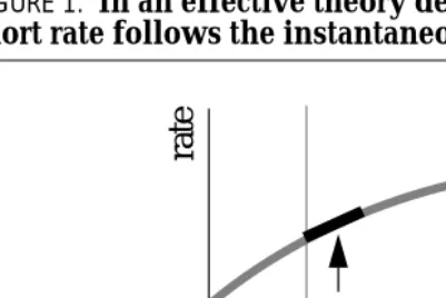
As Figure 1 illustrates, this procedure integrates all sources of inter-est rate stochasticity out of the original theory, and therefore, the effective dynamics of the rates in the effective theory is completely deterministic. As physical time t elapses, the spot rate (or short rate)

r(t) rolls along the static forward rate curve, coinciding with the

for-ward rate at time t:

(EQ 6)

E( )T [ ]…

σ

( )[_σ2( ) ]_T =

E(K T, )[ ]…

The Effective Interest Rate Theory

t≥t0

f_T( )t = f_T

The dynamics of zero-coupon bond prices is also deterministic and is described by a simple backward equation:

(EQ 7)

This equation, with the aid of Equation 6, shows that the asset price dynamics in the effective theory is local and arbitrage-free. Equation 7 is also the dual of the forward equation satisfied by the zero-coupon bond prices:

(EQ 8)

The forward equation is merely a restatement of Equation 1, and holds by the definition of the forward rates regardless of specific assumptions concerning the behavior of interest rates.

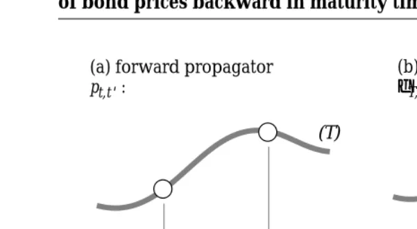
The backward equation describes propagation forward in physical time, for a fixed maturity. More precisely, it relates the prices of a T-maturity bond at different time points t, with earlier times in terms of the later ones. This is best understood by introducing the forward

propagator (or forward Green’s function) pt,t', which relates bond

prices at times t and t', with , for any T-maturity bond, through a simple relationship:

(EQ 9)

The forward propagator p_t,t'describes bond price evolution forward in physical time, as illustrated by Figure 2(a). It satisfies the backward and forward differential equations with boundary conditions p_t,t = 1:

; (EQ 10)

d dt ---– f_t

 

 _B

T( )t = 0

d dT ---+ f_T

 

 _B

T( )t = 0

FIGURE 1. In an effective theory defined by a static forward rate curve, short rate follows the instantaneous forward rates.

0

t

r(t

)

rate

t

r(t

)

time

f

t≤t'

B_T( )t = p_{t t',} B_T( )t'

d dt ---– f_t

 

 _p

t t', = 0 d dt' ---+ f_t'

 

 _p

and for any , the composition relation:

(EQ 11)

Similarly, the forward equation describes propagation backward in maturity time, for a fixed physical time. More precisely, it relates the prices of bonds with different maturities T, but at a fixed time t, with longer maturity bonds in terms of the shorter maturity ones. The

backward propagator11φ_T,T'relates zero-coupon bond prices of matu-rities T and T', with , at any fixed time t, using the relation

(EQ 12)

The backward propagatorφ_T,T' describes bond price evolution back-ward in maturity time, as depicted by Figure 2(b). It also satisfies the forward and backward equations with boundary conditionsφ_T,T = 1:

; (EQ 13)

and, for any , the composition relation

11. The forward and backward propagators for a static yield curve are both simply

equal to the discount function i.e .

t≤ ≤t˜ t'

p t t'( , ) = p t t˜( , )p t˜ t'( , )

p_{u v,} φ_{u v,} f_τdτ

u v

∫

–

 

 

 

exp

= =

T'≤T

B_T( )t = φ_{T T',} B_T'( )t

d dT ---+ f_T

 

 _{ φ}

T T', = 0 d dT' ---– f_T'

 

 _{ φ}

T T', = 0

T'≤ ≤T˜ T

FIGURE 2. Forward propagator describes the evolution of bond prices forward in physical time. Backward propagator describes evolution of bond prices backward in maturity time.

B_T(t) _BT(t')

t t'

(T)

B_T'(t) B_T(t)

T' T

(t)

(a) forward propagator (b) backward propagator

φT,T' :

(EQ 14)

In the effective volatility setting, the local volatility surface is calcu-lated using the spectrum of available option prices (and futures) at time t0, and is assumed to remain unchanged thereafter as time t and

index price S change:

(EQ 15)

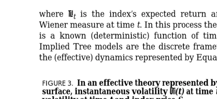
This procedure amounts to averaging out all sources of stochastic vol-atility, leaving the index price uncertainty as the only source of uncertainty left within the theory. The resulting effective dynamics only depends on the index price and time and, as a function of these variables, is deterministic. As the physical time t elapses and index price St moves, the instantaneous volatility σ(t) follows along the

local volatility surface, as depicted in Figure 3, coinciding with the local volatility at time t and level St:

(EQ 16)

This is consistent with an equilibrium (effective) index price process described by the stochastic differential equation:

(EQ 17)

where µt is the index’s expected return and dZt is the standard

Wiener measure at time t. In this process the instantaneous volatility is a known (deterministic) function of time t and index price St.

Implied Tree models are the discrete frameworks for implementing the (effective) dynamics represented by Equation 17. The dynamics of

φT T', = φT T˜, φT˜ T',

The Effective Volatility Theory

σ

σ

FIGURE 3. In an effective theory represented by a static local volatility surface, instantaneous volatilityσ(t) at time t follows the local

volatility at time t and index price St.

t

σ

(t

)

t

σ

(t

)

time

le

v

el

leve l

time vol

local

(t1,S1)

(t2,S2)

σ( )t =

σ

dS_t S_t

standard option prices in the effective theory is described by the

backward equation:

(EQ 18)

Since the only remaining source of uncertainty is the index price, the standard options are completely hedgeable (using index as the hedge) within the effective theory. Equations 16 and 18 then show that the option price dynamics in this theory is arbitrage-free. Equation 18 is also the dual of the forward equation satisfied by the standard option prices:

(EQ 19)

This forward equation is the same as Equation 2 and holds by the definition of local volatility, regardless of any specific assumptions about the behavior of volatility.

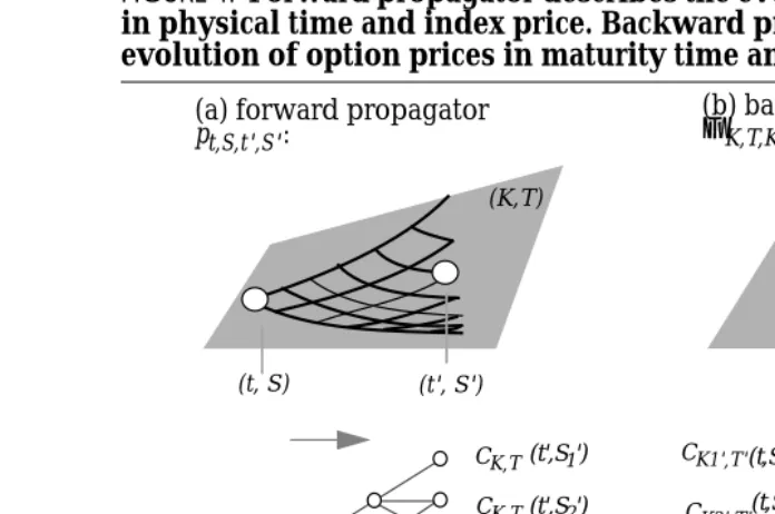
The forward propagator p_t,S,t',S'describes the relationship between the option prices at the two points (t, S) and (t', S'), with , for any

K-strike and T-maturity standard option, through the relation

(EQ 20)

The forward propagator pt,S,t',S' describes option price evolution

for-ward in time and index price, as illustrated by Figure 4(a). We can define the forward transition probability density functionp(t,S,t',S')in terms of the forward propagator as p(t,S,t',S') = er(t'-t) p_t,S,t',S'. It describes the total probability that the index price will reach level S' at time t', given that the index price at time t is S. The mathematical properties ofp_t,S,t',S' andp(t,S,t',S') are discussed in Appendix B.

The backward propagator ΦK,T,K',T' describes the relationship

As Figure 4(b) illustrates, We can also define the effective theory back-ward transition probability density functionΦ(K,T,K',T')in terms of the backward propagator asΦ(K,T,K',T') = eδ(T-T')Φ_K,T,K',T'. Appendix B

dis-cusses some of the mathematical properties ofΦK,T,K',T'andΦ(K,T,K',T').

We can use Equation 17, either by performing simulations or by using implied tree methods, to price and hedge complex options, with the knowledge that the standard options initially used to derive the local volatility surface will have model prices which match their market val-ues. In spite of this calibration, if the volatility has a substantial sto-chastic behavior, the prices and hedge ratios of most options with path-dependent or volatility-path-dependent payoffs will not be accurately repre-sented by the effective theory results. The reason is simply that effec-tive theory results are based on the assumption that local volatilities are static or, equivalently, that the instantaneous volatility is substan-tially a function of the market level (and time). This is a good assump-tion in situaassump-tions where the volatility exhibits strong correlaassump-tion to the market level and, hence, can be viewed predominantly as a function of it. For most equity index option markets, for example, this more or less holds, specially for shorter dated options. On the contrary, in the cur-rency options markets or in longer dated equity (and most other) options markets, the volatility is predominantly stochastic and the effective theory of static local volatilities is not valid. We must there-fore move towards a full stochastic framework by allowing general multi-factor stochastic variations of the volatility surface.

FIGURE 4. Forward propagator describes the evolution of standard prices in physical time and index price. Backward propagator describes the evolution of option prices in maturity time and strike price.

C_K,T

C_K,T

C_K,T C_K,T(t',S₁')

(t',S2')

(t',S_n') (t,S)

...

(K,T)

(t, S) (t', S')

(t,S)

(K, T) (K',T')

C_K,T C_K1',T'

C_K2',T'

C_Kn',T'

... (t,S)

(t,S) (t,S)

(t,S)

(a) forward propagator (b) backward propagator

To allow for stochastic dynamics we must introduce exogenous sto-chastic structure on the effective theory. In general, there are few restrictions on the choice of this structure. One important restriction, which is the cornerstone of the arbitrage framework, is the absence of any explicit future arbitrage opportunities in the final stochastic the-ory. Another restriction is how close the number or the behavior of the stochastic factors are to what is empirically observed. For now, we will consider very general (but sufficiently regular) stochastic struc-tures and discuss the conditions which must be imposed upon them to guarantee the absence of arbitrage. Let us briefly examine the sto-chastic interest rate theory first.

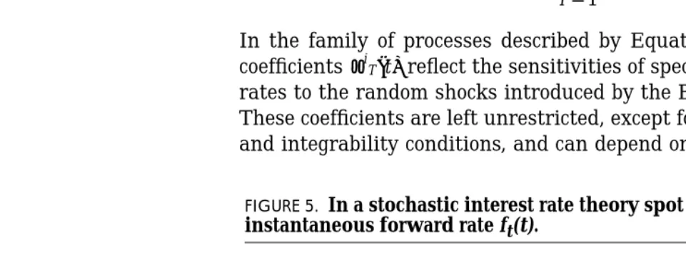
Figure 5 illustrates the dynamics of the forward rates in the stochas-tic framework. Here, the forward rate curve is allowed to fluctuate stochastically with several independent stochastic factors repre-sented by Brownian motions Wi, i = 1, ...,n, with factor volatilities generally depending on both maturity T and time t, according to the stochastic differential equation:

(EQ 22)

In the family of processes described by Equation 22, the volatility coefficients reflect the sensitivities of specific maturity forward rates to the random shocks introduced by the Brownian motions Wi. These coefficients are left unrestricted, except for mild measurability and integrability conditions, and can depend on the past histories of

TOWARDS A STOCHASTIC THEORY OF VOLATILITY

The Stochastic Interest Rate Theory

0

t

r(t

)

rate

r(t

)

time

FIGURE 5. In a stochastic interest rate theory spot rate r(t) follows the instantaneous forward rate f_t(t).

f

(t

)

f

(t

)

T( )t

d f_T( )t α_T( )dtt ϑ_Ti ( )dWt _ti i= 1

n

∑

+ =

the Brownian motions Wi. The drift coefficients must also sat-isfy mild measurability and integrability conditions, but must be fur-ther constrained by the no-arbitrage requirement.

The spot rate at time t, r(t), is the instantaneous forward rate at time

t, i.e, . The stochastic integral equation satisfied by the spot rate is found by integrating Equation 22 and evaluating the result at T = t. It is given by

(EQ 23)

It has been argued by Heath, Jarrow and Morton, that there will be no explicit arbitrage opportunities in the theory defined by Equation 23 if (and only if) the drift coefficients are of the form:

(EQ 24)

Here , i = 1, ..., n, denote the market prices of risk, which can not explicitly depend on maturity T but are otherwise arbitrary. Under these conditions, they have shown that markets are complete and contingent claims prices are independent of the market prices of risk.

Our goal is to introduce a similar stochastic structure on the local volatility surface. To do so, we allow the surface to undergo stochastic fluctuations with several independent stochastic factors, W0, W1, ...,Wn, based on the following stochastic differential equation12:

(EQ 25)

We include W0= Z, the index price’s source of uncertainty, among the

factors so that the stochastic variations of the local volatility surface may depend on the prevailing market level. The family of processes of Equation 25 defines a multi-factor dynamics for the local volatility surface, as illustrated by Figure 6. These processes can be integrated,

12. The variable S in the expression for local volatilityσ_Κ,Τ(t, S)is included for nota-tional purposes and does not imply dependence solely on the spot index level. In fact, local volatilities generally depend on the entire history of the index price and other stochastic factors. Aside from time t and index price S, all other variables have been explicitly omitted from expressions for local volatilities, drifts and factor volatilities.

starting from a fixed (non-random) initial local volatility surface σK,T(0,S0)at time t = 0, as

(EQ 26)

The factor volatility reflects the sensitivity of local volatilities

σ

Brownian motion Wi. Except for mild measurability and integrability conditions13, the family of factor volatilities are unrestricted, generally depending on time and index price, and on the factors or their past histo-ries. However, for the sake of brevity we have omitted explicit references to all variables other than time t and index price S from the expressions for factor volatilities, and we will do the same for other quantities such as drift coefficients and local volatilities.

The spot volatility (or instantaneous volatility) at time t, σ(t), is the

instantaneous local volatility at time t and level S_t, i.e

(EQ 27)

It describes the variability of index price return process, as given by the differential equation

13. The factor volatility functions are assumed to be positive, adapted and

jointly measurable with respect to the Borel σ-algebra restricted to , for

some fixed maximum time T*. They must also satisfy , i = 0, ...,n, to

assure regularity of spot volatility process, and certain additional integrability conditions to assure regularity of the standard option price processes.

FIGURE 6. In a stochastic volatility theory instantaneous volatilityσ(t)

(EQ 28)

or its integral form

(EQ 29)

whereµtis the index’s expected return. Setting T = t and K = St in

Equation 26 we find the stochastic integral equation satisfied by the spot volatility as

(EQ 30)

The drift coefficients must also satisfy mild measurability and integrability conditions, but they must be further restricted by the requirement that the stochastic theory described by Equations 28 and 30 disallows explicit arbitrage opportunities among the standard options, forwards and their underlying index. This is similar to the HJM arbitrage conditions on the spot rate process. Let us briefly examine (a variation of) the HJM argument below.

The bond price dynamics corresponding to the forward rate process of Equation 85 is, by applying Ito’s lemma, described by the stochastic integral equation

(EQ 31)

The symbol here denotes the variational (or functional) derivative with respect to the function f evaluated at u. The first term in this equation describes precisely the effective theory bond price dynamics restricted to the fixed forward rate curve fT(t) at time t. The next two

terms describe the bond price dynamics resulting from the stochastic variations of the effective theory (defined by fT(t)) during the next

infinitesimal time interval dt.

It follows from the definition of the forward rates (Equation 1) that the price of a T-maturity zero-coupon bond with unit face, at time t, is given by

(EQ 32)

From this expression it is simple to see that for any u ( ):

(EQ 33)

Another way of seeing this is by noticing how the forward and back-ward propagators, pt,t'andφT,T', corresponding to an otherwise fixed

(non-random) forward rate curve, respond to sudden changes of a specific forward rate fu along the curve. It is simple to see that pt,t'

satisfies the following relation, as depicted in Figure 7(a):

(EQ 34)

and, as shown in Figure 7(b), thatφ_T,T' satisfies the relation:

(EQ 35)

These relations combined, respectively, with Equations 9 and 12, again lead to Equation 33.

Similarly, we can show that for the second order varia-tional derivatives are given by:

B_T( )t f_u( )t du t

T

∫

–

 

 

exp =

t≤ ≤u T δB_T( )t

δf_u( )t

--- = –BT( )t

FIGURE 7. Sensitivity of the forward and backward propagators pt,t'

andφ_T,T' to the sudden changes of the forward rate f_u.

(a) forward propagator (b) backward propagator

t t'

u -1

t u u+du t' T' u u+du T

T' T

u -1

δp t t'( , ) δf_u

--- = –p(t u, )p u t'( , ) = –p t t'( , )

δφT T', δf_u

--- = –φT u, φu T', = –φT T',

(EQ 36)

The special fu-independent form of variational relations 33-36 can

be directly attributed to the special form of the functional relation-ship between the zero-coupon bond prices and the forward rates as described by Equation 32. This feature underlies the special sim-plicity of no-arbitrage conditions in the HJM framework.

Using Equations 22, 33 and 36 inside Equation 31 we find

(EQ 37)

If the drift coefficients satisfy the no-arbitrage conditions of Equation 24 for some set of market prices of risk , then Equa-tion 37 shows that in terms of the equivalent measure

, defined by the Brownian motions

, i = 1, ..., n, the dynamics of zero-coupon bond prices is:

(EQ 38)

Therefore, {dWi ; i = 1,...,n} defines an equivalent martingale

mea-sure under which the rescaled bond prices for all maturities T are jointly martingale. Under this measure the inter-est rate contingent claims prices are independent of the market prices of risk and, hence, remain preference-free.

The standard option prices CK,T(t,S) are functionals of the local

vol-atilities at time t and market level S, just as bond prices BT(t) are

functionals of the forward rates at time t. As a result, the dynami-cal variations of the lodynami-cal volatility surface induce correpsonding dynamical variations of the standard option prices. During a time interval dt, the index price moves and the local volatilities also change. We can think of the local volatility changes as comprised of two components. A predictable component, due to movements of time and index price restricted to the static local volatility surface

σ

somewhat simpler, but entirely equivalent, to work with the transi-tion probabilities, instead of optransi-tion prices. The transitransi-tion probability,

P_K,T(t,S), describes the total probability that the index price will

reach level K at time T, given that the index price at time t is S, when both the index price and volatility are stochastic. It is related to the option prices C_K,T(t,S) through a general and well-known14 formula:

(EQ 39)

The dynamical evolution of transition probabilities P_K,T(t,S) based on

the local volatility process of Equation 26 is given by the stochastic integral equation:

(EQ 40)

All the probability and local volatility expressions in this equation are evaluated at (t,S). The first term describes the effective dynamics of the transition probabilities PK,T(t,S) restricted to the fixed local

volatility surface

σ

bracket symbol, , therefore, expresses the fact that in this term the future volatility is a deterministic function of the future time T and market level K, given by

σ

these two variables. The next two terms describe the dynamical vari-ations of the transition probabilities resulting from the stochastic fluctuations of the local volatility surface during the next instant of time dt.

Contrary to Equation 32, in general there are no explicit expressions describing the functional relationship between option prices and local volatilities. Therefore, we can not directly compute the variational

14. See Breeden and Litzenberger [1978].

derivatives in Equation 40. Instead, we can look at the variations of the forward and backward transition probabilities with respect to the specific local volatilities. As shown in Appendix C and illustrated in Figure 8, the forward transition probability p(t,S,t',S'), associated with the non-random local volatility surface

σ

time t and spot price S, has the following variational derivative with respect to the local volatility

σ

future maturity u and market level v:

(EQ 41)

FIGURE 8. Sensitivity of the forward and backward transition

probabilities p(t,S,t',S') andΦ(K,T,K',T')to the sudden changes of the local volatility

σ

u v,

( ) (t',S')

t S,

( )

t S,

( ) (t',S')

t S,

( ) (t',S')

u v,

( )

v2 v2

2

∂ ∂

–

K T,

( )

K',T'

( )

K T,

( )

K',T'

( )

v u,

( )

v2 v2

2

∂ ∂

–

K',T'

( ) (v u, ) (K T, )

(a) forward (b) backward

δp t S t' S'( , , , ) δσ2

v u,

--- 1 2

---p t S u v( , , , )v2 v2

2

This relation holds for any u in the range , otherwise the vari-ational derivative is equal to zero. Similarly, the backward transition probability Φ(K,T,K',T') satisfies, for , the relation

(EQ 42)

and zero otherwise. Using Equations 21 and 39, the standard option prices C_K,T(t,S) and transition probabilities P_K,T(t,S) satisfy similar

relationships for :

(EQ 43)

and

(EQ 44)

in which the effective transition probabilities and corre-spond to the static local volatility surface

σ

used the following identities:

(EQ 45)

(EQ 46)

(EQ 47)

As discussed in Appendix B, these identities are all consequences of the fact that the effective theory associated with

σ

all the information necessary for pricing standard options of all strikes and maturities correctly.

for any , and

(EQ 49)

for . Figure 9 gives a graphical depiction of these identi-ties. The standard option prices CK,T(t,S) and transition probabilities PK,T(t,S) satisfy similar relationships for :

(EQ 50)

(EQ 51)

Using these relations, Appendix D proves that Equation 40 leads to

(EQ 52)

if and only if, for any S, K and , the drift functions α_K,T(t,S)

sat-isfy the following no-arbitrage conditions

(EQ 53)

where and for i = 1, ...,n are arbitrary but independent of K and T, and where the equivalent measure { } is defined by

; (EQ 54)

FIGURE 9. Second order variational derivatives of the forward and backward transition probabilities p(t,S,t',S') andΦ(K,T,K',T')with respect to the local volatilities.

K',T'

(a) forward (b) backward

The quantities denote the market prices of risk associated with the volatility risk factors Wi, i = 1, ..., n, whileµ- (r-δ) is the market price

of risk associated with the index price risk factor W0. Equation 52 shows that under the no-arbitrage conditions the measure { ; i =

1, ...,n} is an equivalent martingale measure, with respect to which

the rescaled index price and rescaled option prices for all strikes and maturities are simultaneously martingales.

These no-arbitrage conditions in the present case are significantly more involved than the HJM no-arbitrage conditions described in the previous section. The basic reason is that local volatilities span a (two-dimensional) surface on which (forward and backward) propaga-tion depends, in a rather complicated and non-linear manner, on the structure of local volatilities across the whole surface. This is evident by the apparent complexity of Equations 44 and 51 as compared to the simplicity of the corresponding Equations 33 and 36 in the inter-est rate framework. It is, therefore, rather difficult to use the no-arbi-trage conditions for stochastic volatility in their continuous form directly.

In the next section we introduce Stochastic Implied Trees as a dis-crete-time framework for describing arbitrage-free stochastic varia-tions of the local volatility surface.

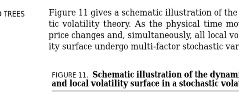
Figure 11 gives a schematic illustration of the dynamics in a stochas-tic volatility theory. As the physical time moves forward, the index price changes and, simultaneously, all local volatilities on the volatil-ity surface undergo multi-factor stochastic variations.

Πi

dWi

StOCHASTIC IMPLIED TREES

FIGURE 11. Schematic illustration of the dynamics of the index price and local volatility surface in a stochastic volatility theory.

To provide a more quantitative description of this stochastic dynamics we choose to work within a discrete-time framework described by a Stochastic Implied Tree. These trees are extensions of the standard (non-stochastic) implied trees, which are used to describe effective volatility models (see Derman, Kani and Chriss [1996]). Figure 12 shows an example of a 1-year, 5-period standard implied trinomial tree which is calibrated to a market where at-the-money implied volatility is 25% and there is an implied volatility skew of 0.5% point per 10 strike points. In an implied trinomial tree

FIGURE 12. Example of an Implied Trinomial Tree describing an effective volatility theory.

100.00

83.80 119.34 119.34 119.34 119.34

100.00 100.00 100.00 100.00 142.41 142.41 142.41

the location of the nodes, or the state space, is more or less arbitrarily. Once the state space is fixed, however, the transition probabilities at different nodes are determined from the requirement that standard options and forwards with strike prices coinciding with those nodes and maturing at different periods of the tree all have prices using the tree which match their market prices. Since local volatility at any node depends on the nodal levels and the transition probabilities to the nearby nodes, the local volatilities at different nodes are also determined in this way.

Stochastic implied trinomial trees are extensions of the implied trino-mial tree in which the transition probabilities are, in addition, allowed to vary stochastically, with several stochastic factors, as time elapses and index level moves. The index level is allowed to move randomly from node to node, while the local volatilities, and simulta-neously the transition probabilities corresponding to the future nodes, all vary stochastically across the tree. This behavior is shown in Figure 13.

Starting from any initial node, the possible future movements of the local volatility surface must be restricted to guarantee absence of any arbitrage opportunities in the discrete theory represented by the sto-chastic implied tree. As discussed earlier, this is equivalent to the requirement that the total transition probabilties to all future nodes be simultaneously martingales on the tree. This is also the same as FIGURE 13. In a Stochastic Implied Tree, as the index moves from node A to node B in a single time step, the local volatilities and transition probabilities, for every node on the future subtree beginning at node B, vary stochastically with multiple stochastic factors.

A

the requirement that all rescaled standard option prices be simulta-neously martingales on the tree. As Figure 14 shows, during the time interval∆t, the spot price will move randomly (by amount∆S) to one

of the nearby nodes and, at the same time, the local volatility surface will assume one of its N possible configurations, w1, ...,wN. As a result, the total transition probability P_K,T(t,S) to any given future

node (K,T) also moves to one of its several possible values P(i)_K,T(t+∆t, S+∆S), i = 1, ..., M, during this time interval. To guarantee

no-arbi-trage, P_K,T must be a martingale (fair game), that is it must equal the expectation , under some (equivalent) measure, of its future val-ues P(i)_K,Tfor all the future nodes (K,T) on the tree.

To make positivity manifest, it is more convenient to redefine the drift and volatility functions in Equation 25 as and , l = 0, ..., n, and begin by discretizing the following continuous-time differential equation:

(EQ 55)

We let the integer pair (i,j) label the node (ti,Sj) describing the

cur-rent location (i.e (t,S)) of the index at the ithstep of the simulation.

t

t +

∆

t

P

P

P

randomly to one of the nearby nodes and the local volatility surface assumes one of N possible configurations.

t

t +

∆

t

w

w1

wN

Our Notation in Discrete Time

αK T, αK T, σK T, 2 → θl

K T, θlK T, σK T, 2 →

dσ2

K T, (t S, )

σ2

K T, (t S, )

--- α_{K T,} (t S, )dt θl

K T, (t S, )dWtl l=0

n

∑

We also let the pair (n,m) label the future node (t_n,S_m) corresponding

the future time and level (i.e (T,K)). Then the discrete form of Equa-tion 55 can be written as

(EQ 56)

The vector (∆W_i0,∆W_i1, ...,∆W_in) is random and is drawn, at time i,

from the sample space of the increments of n independent Brownian motions Wl.

The volatility parameters are pre-specified but the drift parameters must be determined from the no-arbitrage requirements that the total probabilities of arriving at the future node (n,m) from the (fixed) initial node (i,j) must be jointly martingales for all future nodes (n,m). As we shall argue below, these martingale conditions are precisely enough to completely determine all the drift parameters step by step during the simulation process.

A Stochastic Implied Tree simulation begins with the construction of a trinomial implied tree calibrated to today’s prices of standard options and forwards. The simulation begins at the node (0,0) of this tree. During the first simulation step the drift parameters , for all future nodes (m,n), are determined from the martingale condi-tions on the total probabilities . Figure 15 illustrates that

∆σ2

m n, ( )i j, σ 2

m n, ( ) αi j, m n, ( )∆ti j, i θm n, l

i j, ( )∆Wi

l

l=0 n

∑

+ =

θm n, l

i j, ( ) αm n, ( )i j,

P_{m n,} ( )i j,

αm n, (0 0, )

P_{m n,} (0 0, )

FIGURE 15. The drift parameterα0,0(0,0) in a Stochastic Implied Tree is determined from the martingale condition on the total transition probability P1,2(0,0).

(0,0) (1,2)

(0,0) (1,2)

(0,0) (1,2)

a

(0,0)

the drift parameter is determined from the martingale con-dition for This also guarantees that the transition probabili-ties and are martingales. The reason is that these probabilities are constrained by two extra conditions which must hold irrespective of the specific behavior of the local volatilities:

(EQ 57)

The first condition is the normalization condition, requiring that the sum of the three total transition probabilities at time t1 must be

unity. The second is the forward condition, requiring that the t1

-maturity forward price at time t0 must match its risk-neutral value.

In a similar way, the three drift parameters , and are determined from the martingale conditions of the three

total transition probabilities , and . The

remaining transition probabilities and will then also be martingales due to the normalization and forward conditions at time t2. In this way all drift parameters will be

deter-mined during the first simulation step. Finally, to complete this step we draw a random vector (∆W00, ∆W01, ..., ∆W0n) from the sample

space of the increments of Wiat time t0, and use this vector to

simul-taneously arrive at a (random) new location for the index price and new values for all future local volatilities. Equation 56 is used directly with i = j = 0 to calculate the new local volatility values from this choice of the random vector. As for the index price, we use the random number∆W00to determine which of the three possible future

nodes (i.e (1,2), (1,1) or (1,0)) does the index price moves to during time interval ∆t. Figure 16 gives one simple possible method for

α0 0, (0 0, ) P_{1 2,} (0 0, )

P_{1 1,} (0 0, ) P_{1 0,} (0 0, )

P1 0, (0 0, )+P1 1, (0 0, )+P1 2, (0 0, ) = 1

P1 0, (0 0, )S1 0, +P1 1, (0 0, )S1 1, +P1 2, (0 0, )S1 2, S0 0, e r–δ ( )(t₁–t₀) =

α1 2, (0 0, ) α1 1, (0 0, ) α1 0, (0 0, )

P2 4, (0 0, ) P2 3, (0 0, ) P2 2, (0 0, ) P2 1, (0 0, ) P2 0, (0 0, )

αm n, (0 0, )

FIGURE 16. Determining which node the index price will go to during one simulation step using the renormalized random number∆Wi0.

(i, j)

(i+1, j+2) if∆W_i0 >= P_m + P_d

(i+1, j+1) if∆W_i0>= P_d and∆W_i0 < P_m + P_d

(i+1, j) if∆W_i0< P_d P_u = P_u(i,j)

doing this starting from an arbitrary initial node (i,j). First∆W_i0 is renormalized to represent a uniformly-distributed random number between 0 and 1. Let P_u(i,j), P_m(i,j) and P_d(i,j) denote the one period

transition probabilities, prevailing at time t_i and index price S_j, from the node (i,j) to the up, middle and down nodes at time t_i+1. We then compare our random number with these three probabilities. If it is smaller than P_d(i,j), we move the index price to the down node. On

the other hand, if the random number is greater than the sum P_u(i,j) + P_m(i,j), we allow the index price to move to the up node. In every

other case we move the index price to the middle node at the next time period.

We can continue this procedure, step-by-step, for any point (i,j) along a simulated path through the stochastic implied tree. First, all the drift parameters are determined from the martingale condi-tions on . Appendix E gives the necessary details for doing this calculation. Subsequently, these drift parameters are used to generate arbitrage-free (random) movements of the future local vola-tility surface as the index price moves randomly forward across the tree. We can generate many such sample paths through the tree. Along each path, the movements of the index price and the local vola-tility surface are random realizations of an arbitrage-free dynamics, which step-by-step guarantees absence of arbitrage opportunities among different standard option (and forward) contracts and their underlying index within the discrete time framework of the stochas-tic implied tree.

Consider a one-factor stochastic volatility model with a lognormal volatility of volatility structure, as described by the following pair of stochastic differential equations:

where . For the purpose of this example we take the volatility coefficient to be constant, so that the factor W1 has the interpretation of a simultaneous constant (proportional) shift in all local volatilities. All the other quantities can depend on t, S, factors

W0 and W1 or their past values. More specifically, we consider a 1-year, 5-period example with the initial term and strike structure of

αm n, ( )i j, P_{m n,} ( )i j,

A SIMPLE EXAMPLE

dS S

--- = µdt+σdW0 dσ2K T,

σ2 K T,

--- = αK T_, dt+θdW1 σ( )t σ_{t S}

t , (t S, t) =

volatility given by an at-the-money implied volatility of 20% and a constant skewness of 0.5% per 10 strike points. For instance, ini-tially a 80 strike option of any maturity has implied volatility of 21%. Let the riskfree discount rate be equal to 10%, dividend yield 5% and the volatility (of volatility) parameter = 30%. We choose the state space of the stochastic implied trinomial tree to be the same as a standard (CRR- type) trinomial tree with constant vola-tility of 20%. Figure 17 shows this state space. It also shows the local volatilities and total transition probabilities, corresponding to various nodes of this tree, at the initial time t = 0. As we expect,

θ

FIGURE 17. The state space of a Stochastic Implied Trinomial Tree, the local volatility surface and the total transition probability distribution on the tree at the initial time t = 0.

100.00

86.81

115.19 115.19 115.19 115.19

100.00 100.00 100.00 100.00

132.69 132.69 132.69

75.36 75.36 75.36

152.85 152.85

65.43 65.43

56.80 176.06

86.81 86.81

86.81 state space:

0.199

0.191 0.189 0.188

0.199 0.197 0.197

0.180 0.177

0.251 0.240

0.155

0.263 0.211 0.215

0.218 . local vols

σ

1.000

0.182

0.275 0.281 0.267 0.251

0.493 0.376 0.311 0.271

0.071 0.112 0.135

0.066 0.070 0.083

0.016 0.037

0.026 0.028

0.011 0.003

0.197 0.206

local volatilities increase as the index level decreases roughly twice as fast as implied volatilities. Also the probability distribution is skewed (around the forward price) towards the lower index levels. The first step toward the construction of the stochastic implied tree is to determine the drift coefficients at time t₀= 0. Appendix E

gives the formulas for directly calculating these coefficients, which αm n, (0 0, )

FIGURE 18. The first step of the Stochastic Implied Tree construction consists of determining all the drift coefficientsαm,n(0,0), at time t0=

0, from the martingale conditions for the total probabilities P_m,n(0,0).

1.000

0.182

0.275 0.281 0.267 0.251

0.493 0.376 0.311 0.271

0.071 0.112 0.135

0.066 0.070 0.083

0.016 0.037

0.026 0.028

0.011 0.003

0.197 0.206

0.232 total probs P_m,n(0,0):

-0.044

-0.184 -0.037 0.009

0.139 0.072 0.063

-0.298 -0.194

-0.369 -0.195 -0.381

-0.452 -0.043 -0.051

-0.232 drifts

α

choose a random vector (∆W0,∆W1) -> (up, up) 0.199

0.191 0.189 0.188

0.199 0.197 0.197

0.180 0.177

0.251 0.240

0.155

0.263 0.211 0.215

0.218 . local vols

σ

are shown in Figure 18. We can justify the numbers by examining what can happen to the total transition probabilities during the next time interval∆t. All local volatilities will simultaneously move, with

probability of 1/2, to their up values, , or their down

val-ues, , as given by

1.000

0.175

0.343 0.278 0.243 0.220

0.346 0.303 0.256 0.226

0.103 0.142 0.154

0.206 0.284 0.291 0.282

0.640 0.448 0.367 0.315

0.038 0.082 0.116

0.275 0.281 0.267 0.251

0.493 0.376 0.311 0.271

0.071 0.112 0.135

average total probs (P(u)_m,n(0,0)+P(d)_m,n(0,0))/2:

FIGURE 19. Up- and down- values of local volatilities and total transition probabilities corresponding the first simulation step.

with given in Figure 18. As a result, all transition probabil-ities also change across the tree, simultaneously moving to their up values, , or to their down values, , each with probability of 1/2. Figure 19 shows that with the present choice of drift coefficients the initial total probabilities are precisely equal to the average value of their up and down values. To complete the step 1 we draw a pair of independent random numbers between 0 and 1, say

αm n, (0 0, )

P( )um n, (0 0, ) P( )dm n, (0 0, )

FIGURE 20. During the step 2 of the simulation, the drift coefficients α_m,n(1,2), at time t₁ = 0.25, are determined from the martingale

conditions for the total probabilities Pm,n(1,2).

0.210 0.215 0.216

0.231 0.230

0.192 0.194

0.161

0.240 local vols

σ

0.089

1.000 0.436 0.336 0.273

0.363 0.205 0.193

0.301 0.296 0.271

0.030

0.077 0.129

0.015

0.085 total probs P_m,n(1,2):

-0.044 0.189 0.051

-0.229 0.016 -0.186 -0.017

-0.299

-0.365 drifts

α

choose a random vector (∆W0,∆W1) -> (middle, down)

(0.853, 0.612). Since 0.853 is greater than the sum of prevailing down and middle probabilities, 0.493+0.232 = 0.725, as discussed in Figure 16 we move the index to the node (1,2). Also, since 0.612 is greater than 1/2 we move all local volatilities to their up values, before we begin the next simulation step. The step 2 of the

simula-FIGURE 21. During the step 3 of the simulation, the drift coefficients αm,n(2,3), at time t2 = 0.50, are determined from the martingale

conditions for the total probabilities Pm,n(2,3).

0.192 0.186

0.197 0.164 local vols

σ

0.048

1.000 0.529 0.389

0.213 0.213

0.258 0.298

0.051 0.001

total probs P_m,n(2,3):

-0.044 0.113 -0.235 -0.182 drifts

α

choose a random vector (∆W0,∆W1) -> (up, up)

tion is precisely the same as step 1, except confined to the subtree that begins at the node (1,2). As shown in Figure 20, again the mar-tingale conditions on the total probabilities are used to solve for the drift coefficients at time t₁ = 0.25, and then

these coefficients, together with a pair of random numbers, are used to determine jointly the new values for the index price and the future

P_{m n,} (1 2, ) αm n, (1 2, )

FIGURE 22. During the step 4 of the simulation, the drift coefficients α_m,n(3,5), at time t₃ = 0.75, are determined from the martingale

conditions for the total probabilities Pm,n(3,5).

0.180 local vols

σ

0.183

1.000 0.584

0.232 total probs P_m,n(3,5):

-0.044 drifts

α

choose a random vector (∆W0,∆W1) -> (down, - )

local volatilities. Steps 3 and 4 are also quite similar and their results have been shown in Figures 21 and 22, repsectively.

In this example, we chose a simple two-state (up and down) repre-sentation for the stochastic movements of the local volatility sur-face during the time step . We could instead choose any equivalent representation of the same process with m states, for any integer m > 1. There are infinite number of equivalent repre-sentations for any choice of m. If the model is well-behaved, these discrete representations should all converge to the same continu-ous-time process as goes to zero. However, a representation with large number of states may converge substantially faster than the two-state representation we chose here. Table 1 shows the calibra-tion results for a 50000 path simulacalibra-tion on the 5-period tree described above.

TABLE 1.Calibration results of a 50000-path simulation on a 1-year, 5-period Stochastic Implied Tree.

The fourth and fifth columns give, respectively, the standard (non-stochastic) implied trinomial tree and the Stochastic Implied Tree results for a series of standard European-style call and put options used to calibrate the trees. The results are seen to agree well.

Strike Price

Option Type

Black-Scholes

Price

Standard Implied Tree Price

Stochastic Implied Tree Price

130 call 1.142 1.118 1.176

120 call 2.629 2.764 2.775

110 call 5.332 5.529 5.556

100 call 9.628 9.395 9.432

90 put 2.452 2.566 2.556

80 put 0.840 0.936 0.928

70 put 0.202 0.244 0.230

∆t

CAVIAT: Since the location of the nodes (i.e the state space) of the stochastic implied trinomial tree is fixed throughout, it may not be possible to fit very large local volatilities, which may occur at various nodes and at different times during the simulation, with transition probabilities which lie between 0 and 1. In such cases, we must

over-write the unacceptable transition probabilities (or, equivalently, the

local volatilities) at those nodes15. Even though, this overwrite proce-dure makes for an imperfect calibration to the initial smile (and, the-oretically, a violation of arbitrage), it must be diligently adhered to, in order to keep the simulation process meaningful. We can define overwrite ratio as the number of overwrites per future node, per sim-ulation path. In the previous example, the overwrite ratio for 5 peri-ods and 50000 paths is found to be 2.7%, indicating that only a relatively small portion of the calculated local volatilities have been overwritten.

Consider a realized variance forward contract16, defined as a forward contract on the realized variance of index returns, , with strike price K and payoff at the contract maturity. Table 2 shows the valuation results for a 1-year realized variance contract with zero strike price, using 20-period, 10000 path stochastic implied tree sim-ulations with four different volatility of volatility parameters θ =0%, 20%, 30%, 50%.To make the results more clear, we choose a flat ini-tial volatility smile with a constant implied volatility of 20% for all standard European options. Also the discount rate and dividend yield are both chosen to be zero.

TABLE 2.Prices of a zero-strike realized variance forward contract for different values of the volatility of volatility parameter.

It is clear from this table that the price of a realized variance forward contract is independent of the volatility of volatility parameter, and is

15. This also occurs in the standard implied trees. See, for instance, Derman, Kani and Chriss [1996].

16. See also Investing in Volatility, Derman etal. [1996].

θ 0% 20% 30% 50%

price 399.81 400.37 401.10 400.69

Pricing of Some Contracts with Payoffs Based on Realized Volatility

Σ2 Σ2

K –

what one would expect from a static 20% flat initial implied volatility surface. In fact, it can be shown that under very general conditions (see footnote 14) the price of this forward contract depends only on the initial volatility surface and not on the specific stochastic aspects of the volatility process. More precisely, it’s price equals the dis-counted value of the expected (equilibrium) total index return vari-ance during the life of the contract. As discussed earlier, this expectation is fully embodies in today’s local volatility surface. There-fore, we are able to price this forward contract by using an effective theory (θ = 0), as the second column in the table indicates. This is

quite analogous to our ability to price ind