Word Sense Disambiguation using Static and Dynamic Sense
Vectors
Jong-Hoon Oh, and Key-Sun Choi
Computer Science Division, Dept. of EECS, Korea Advanced Institute of Science & Technology (KAIST) / Korea Terminology Research Center for Language and Knowledge Engineering
(KORTERM), 373-1, Guseong-dong, Yuseong-gu, Daejeon, 305-701, Korea Email: {rovellia,kschoi}@world.kaist.ac.kr
Abstract
It is popular in WSD to use contextual information in training sense tagged data. Co-occurring words within a limited window-sized context support one sense among the semantically ambiguous ones of the word. This paper reports on word sense disambiguation of English words using static and dynamic sense vectors. First, context vectors are constructed using contextual words1 in the training sense
tagged data. Then, the words in the context vector are weighted with local density. Using the whole training sense tagged data, each sense of a target word2 is represented
as a static sense vector in word space, which is the centroid of the context vectors. Then contextual noise is removed using a automatic selective sampling. A automatic selective sampling method use information retrieval technique, so as to enhance the discriminative power. In each test case, a automatic selective sampling method retrieves N relevant training samples to reduce noise. Using them, we construct another sense vectors for each sense of the target word. They are called dynamic sense vectors because they are changed according to a target word and its context. Finally, a word sense of a target word is determined using static and dynamic sense vectors. The English SENSEVAL test suit is used for this experimentation and our method produces relatively good results.
1 ‘Contextual words’ is defined as a list of content
words in context.
2 In this paper, a target word ‘Wt’ is a semantically
1. Introduction
It is popular in WSD to use contextual information in training data (Agirre, et al., 19963; Escudero, et al., 2000; Gruber, 1991;
Schutze, 1998). Co-occurring words within a limited window-sized context support one sense among the semantically ambiguous ones of the word. The problem is to find the most effective patterns in order to capture the right sense. It is true that they have similar context and co-occurrence information when words are used with the same sense (Rigau, et al., 1997). It is also true that contextual words nearby an ambiguous word give more effective patterns or features than those far from it (Chen, et al., 1998). In this paper, we represent each sense of a word as a vector in word space. First, contextual words in the training sense tagged data4 are represented as context vectors. Then,
ambiguous word in a given context of ‘Wt’. This context may consist of several sentences and it is represented by ‘contextual words’.
3 Agirre et al., (1996) defines a term ‘conceptual
density’ based on how many nodes are hit between WordNet node and target words+contexts. Unlike ‘Conceptual density’, ‘local density’ used in this paper does not use any semantic net like WordNet but use only the contextual words surrounding the given target word..
4 In this paper, the English SENSEVAL-2 data for
the words in the context vector are weighted with local density. Then, each sense of a target word can be represented as a sense vector, which is the centroid of the context vectors in word space.
However, if training samples contain noise, it is difficult to capture effective patterns for WSD (Atsushi, et al., 1998). Word occurrences in the context are too diverse to capture the right pattern for WSD. It means that the dimension of contextual words will be very large when we will use all words in the training samples for WSD. To avoid the problems, we use an automatized hybrid version of selective sampling that will be called “automatic selective sampling”. This automatization is based on cosine similarity for the selection. For a given target word and its context, this method retrieves N-best relevant training samples using the cosine similarity. Using them, we can construct another sense vectors for each sense of the target word. The relevant training samples are retrieved by comparing cosine similarities between given contexts and indexed context vectors of training samples. The ‘automatic selective sampling’ method makes it possible to use traning samples which have higher discriminative power.
This paper is organized as follows: section 2 shows details of our method. Section 3 deals with experiments. Conclusion and future works are drawn in sections 4.
2 Word Sense Disambiguation Method
2.1 Overall System Description
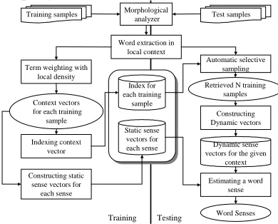
Figure 1 shows the overall system description. The system is composed of a training phase and a test phase. In the training phase, words in the limited context window of training samples, which contains a target word and its sense, are extracted and the words are weighted with local density concept (section 2.2). Then, context vectors, which represent each training sample, are indexed and static sense vectors for each a target word , its sense and its context. But the sense of contexual words is not annotated in the training samples (SENSEVAL-2, 2001)
sense are constructed. A static sense vector is the centroid of context vectors of training samples where a target word is used as a certain sense (section 2.3). For example, two sense vectors of ‘bank’ can be constructed using context vectors of training samples where ‘bank’ is used as ‘business establishment’ and those where ‘bank’ is used as ‘artificial embankment’. Each context vector is indexed for ‘automatic selective sampling’.
Training samples
Word extraction in local context Term weighting with
local density
Indexing context vector Context vectors for each training
sample
Constructing static sense vectors for
each sense
Index for each training
sample Static sense vectors for each sense
Automatic selective sampling
Estimating a word sense Dynamic sense vectors for the given
context Test samples
Word Senses Constructing Dynamic vectors Retrieved N training
samples
Training Testing Morphological
analyzer
Fig. 1 The overall system description
In the test phase, contextual words are extracted with the same manner as in the training phase (section 2.5). Then, the ‘automatic selective sampling’ module retrieves top-N training samples. Cosine similarity between indexed context vectors of training samples, and the context vector of a given test sample provides relevant training samples. Then we can make another sense vectors for each sense using the retrieved context vectors. Since, the sense vectors produced by the automatic selective sampling method are changed according to test samples and their context, we call them dynamic sense vectors in this paper (section 2.4) (Note that, the sense vectors produced in the training phase are not changed according to test samples. Thus, we call them static sense vectors.)
The similarities between dynamic sense vectors, and a context vector of a test sample, and those between static sense vectors and the context vector of the test sample are estimated by cosine measure. The sense with the highest similarity is selected as the relevant word sense.
Our proposed method can be summarized as follows
1) Constructing context vectors using contextual words in training sense tagged data.
2) Local density to weight terms in context vectors.
3) Creating static sense vectors, which are the centroid of the context vectors.
Test Phase
1) Constructing context vectors using contextual words in test data.
2) Automatic selective sampling of training vectors in each test case to reduce noise.
3) Creating dynamic sense vectors, which are the centroid of the training vectors for each sense. 4) Estimating word senses using static
and dynamic sense vectors.
2.2 Representing Training Samples as a Context Vector with Local Density
In WSD, context must reflect various contextual characteristics5. If the window size of context is
too large, the context cannot contain relevant information consistently (Kilgarriff et al., 2000). Words in this context window6 can be classified
into nouns, verbs, and adjectives. The classified words within the context window are assumed to show the co-occurring behaviour with the target word. They provide a supporting vector for a certain sense. Contextual words nearby a target word give more relevant information to decide its sense than those far from it. Distance from a target word is used for this purpose and it is calculated by the assumption that the target words in the context window have the same sense (Yarowsky, 1995).
Each word in the training samples can be weighted by formula (1). Let Wij(tk) represent a
weighting function for a term tk, which appears
in the jth training sample for the ith sense, tfijk
5 POS, collocations, semantic word associations,
subcategorization information, semantic roles, selectional preferences and frequency of senses are useful for WSD (Agirre et al., 2001).
6 Since, the length of context window was
considered when SENSEVAL-2 lexical sample data were constructed, we use a training sample itself as context window.
represent the frequency of a term tk in the jth
training sample for the ith sense, dfik represent
the number of training samples for the ith sense where a term tk appears, Dijk represent the
average distance of a term tk from the target
word in the jth training sample for the ith sense, and Ni represent the number of training samples
for the ith sense.
In formula (1), Z is a normalization factor, which forces all values of Wij(tk) to fall into
between 0 and 1, inclusive (Salton et al., 1983). Formula (1) is a variation of tf-idf. We regard each training sample as indexed documents, which we want to retrieve and a test sample as a query in information retrieval system. Because we know a target word in training samples and test samples, we can restrict search space into training samples, which contain the target word when we find relevant samples. We also take into account distance from the target word. Dijk and dfik in formula (1) support a local
density concept. In this paper, ‘local density’ of a target word ‘Wt’ is defined by the density among contextual words of ‘Wt’ in terms of their in-between distance and relative frequency. First, the distance factor is one of the important clues because contextual words surrounding a target word frequently support a certain sense: for example, ‘money’ in ‘money in a bank’.
Second, if contextual words frequently co-occur with a target word of a certain sense, they may be a strong evidence to decide what word sense is correct. Therefore, contextual words, which more frequently appear near a target word and appear with a certain sense of a target word, have a higher local density.
with context words and their weight, such that (wij(t1),wij(t2),….,wij(tn)). When Wij(tk) is 1, it
means that tk is strong evidence for the ith sense.
(Zijk are much larger than others.)
2.3 Constructing Static Sense Vectors
Now, we can represent each training sample as context vectors using contextual words such that vij=(wij(t1),wij(t2),….,wij(tn)) where vij represents a
context vector of the jth training sample for the ith sense and wij(tk) is the weight of a term tk
calculated by formula (1).
| |
| |
1
i N
j ij
i N
v SV
i
∑
== (2)
Context vectors for Sense 1 Context vectors
for Sense 2
Context vector for Sense n
…
2
SV
1
SV
n
SV
Fig.2 A graphical representation of static sense vectors
Throughout clustering the context vectors, each sense can be represented as sense vectors. Let Ni
represent the number of training samples for the ith sense, and vij represent the context vector of
the jth training sample for the ith sense. The static sense vector for the ith sense, SVi, can be
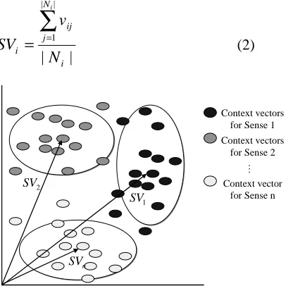
represented by formula (2) (Park, 1997). In formula (2), SVi is the centroid of context
vectors of training samples for the ith sense as shown in figure 2. In figure 2, there are n senses and context vectors, which represent each training sample. We can categorize each context vector according to a sense of a target word. Then, each sense vectors are acquired using formula (2). Because the sense vectors are not changed according to test samples, we call them a static sense vector in this paper (note that sense vectors, which we will describe in section 2.4, are changed depending on the context of test
samples).
2.4 Automatic selective sampling: Dynamic Sense Vectors
It is important to capture effective patterns and features from the training sense tagged data in WSD. However, if there is noise in the training sense tagged data, it makes difficult to disambiguate word senses effectively. To reduce its negative effects, we use a automatic selective sampling method using cosine similarity. Figure 3 shows the process of a automatic selective sampling method. The upper side shows retrieval process and the lower side shows a graphical representation of dynamic sense vectors.
Sense 1 Sense 2 Sense n
..
Retrieved Training Samples
.. ..
A target word
DSV1 DSV2 DSVn
…
… A Context vector for a test sample
Indexed Training Samples
Context vectors for Sense 1 Context vectors
for Sense 2
Context vectors for Sense n
…
2
DSV
1
DSV
n
DSV
A context vector of a test sample Retrieved top-N
training sample
Fig. 3 A graphical representation of an automatic selective sampling method
training samples can be clustered as Dynamic Sense Vectors according to a sense of their target word. Since, the sense vectors produced by a automatic selective sampling method are changed according to the context vector of a test sample, we call them dynamic sense vectors in this paper.
Let RTi represent the number of training samples
for the ith sense in the retrieved top-N, and vij
represent a context vector of the jth training sample for the ith sense in the top-N. The dynamic sense vector for the ith sense of a target word, DSVi, is formulated by formula (3). In
formula (3), DSVi means the centroid of the
retrieved context vectors of training samples for the ith sense as shown in the lower side of
2.5 Context Vectors of a Test Sample
Contextual words in a test sample are extracted as the same manner as in the training phase. The classified words in the limited window size – nouns, verbs, and adjectives – offer components of context vectors. When a term tk appears in the
test sample, the value of tk in a context vector of
the test sample will be 1, in contrary, when tk
does not appear in the test sample, the value of tk
in a context vector of the test sample will be 0. Let contextual words of a test sample be ‘bank’, ‘river’ and ‘water’, and dimension of context vector be (‘bank’, ‘commercial’, ‘money’, ‘river’, ‘water’). Then we can acquire a context vector, CV =(1,0,0,1,1), from the test sample. Henceforth we will denote CVi as a context
vector for the ith test sample.
2.6 Estimating a Word Sense: Comparing Similarity
We described the method for constructing static sense vectors, dynamic sense vectors and context vectors of a test sample. Next, we will describe the method for estimating a word sense using them. The similarity in information retrieval area is the measure of how alike two documents are, or how alike a document and a query are. In a vector space model, this is usually interpreted as how close their
corresponding vector representations are to each other. A popular method is to compute the cosine of the angle between the vectors (Salton et al., 1983). Since our method is based on a vector space model, the cosine measure (formula (4)) will be used as the similarity measure. Throughout comparing similarity between SVi
and CVj and between DSVi and CVj for the i th
sense and the jth test sample, we can estimate the relevant word sense for the given context vector of the test sample. Formula (5) shows a combining method of sim(SVi,CVj) and
sim(DSVi,CVj). Let CVj represent the context
vector of the jth test sample, si represent the ith
sense of a target word, and Score(si,CVj)
represent score between the ith sense and the context vector of the jth test sample.
∑
where, N represents the dimension of the vector space, v and w represent vectors.
Because the value of cosine similarity falls into between 0 and 1, that of Score(si,CVj) also exists
between 0 and 1. When similarity value is 1 it means perfect consensus, in contrary, when similarity value is 0 it means there is no part of agreement at all. After all, the sense having maximum similarity by formula (5) is decided as the answer.
3. Experiment
3.1 Experimental Setup
In this paper, we compared six systems as follows.
The system that assigns a word sense which appears most frequently in the training samples (Baseline)
The system that is trained by co-occurrence information directly without changing. (only with term frequency) (B)
The system with local density and without automatic selective sampling (C)
The system with automatic selective sampling and without local density (D) The system with local density and
automatic selective sampling (E) System A was used to compare our method with the other method. System B, C, D, and E will show the performance of each component in our proposed method. To evaluate performance in the condition of ‘without local density (system B and D)’, we weight each word with its frequency in the context of training samples.
The test suit used is the English lexical samples released for SENSEVAL-2 in 2001. This test suit supplies training sense tagged data and test data for noun, verb and adjective (SENSEVAL-2, 2001).
Cross-validation on training sense tagged data is used to determine the parameters –
λ
in formula (5) and top-N in constructing dynamic sense vectors. We divide training sense tagged data into ten folds with the equal size, and determine each parameter, which makes the best result in average from ten-fold validation. The values, we used, areλ
=0.2, and N =50. The results were evaluated by precision rates (Salton, et al., 1983). The precision rate is defined as the proportion of the correct answers to the generated results.3.2 Experimental Results
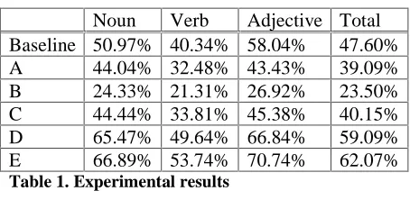
Noun Verb Adjective Total Baseline 50.97% 40.34% 58.04% 47.60% A 44.04% 32.48% 43.43% 39.09% B 24.33% 21.31% 26.92% 23.50% C 44.44% 33.81% 45.38% 40.15% D 65.47% 49.64% 66.84% 59.09% E 66.89% 53.74% 70.74% 62.07%
Table 1. Experimental results
Table 1 shows experimental results. In the result , all systems and baseline show higher performance on noun and adjective than verb. This indicates that the disambiguation of verb is more difficult than others in this test suit. In
analysing errors, we found that we did not consider important information for disambiguating verb senses such as adverbs, which can be used as idioms with the verbs. For example, ‘carry out’, ‘pull out’ and so on. It is necessary to handle them for more effective WSD.
System B, C, D, and E show how effective local density and dynamic vectors are in WSD. The performance increase was shown about 70% with local density (system C) and about 150% with dynamic vectors (system D), when they are compared with system B – without local density and dynamic vectors. This shows that local density is more effective than term frequency. This also shows that automatic selective sampling of training samples in each test sample is very important.
Combining local density and dynamic vectors (system E), we acquire about 62% performance. Our method also shows higher performance than baseline and system A (the Naïve Bayesian method) – about 30% for baseline and about 58% for system A.
As a result of this experiment, we proved that co-occurrence information throughout the local density and the automatic selective sampling is more suitable and discriminative in WSD. This techniques lead up to 70% ~ 150% performance improvement in the experimentation comparing the system without local density and automatic selective sampling.
4. Conclusion
This paper reported about word sense disambiguation for English words using static and dynamic sense vectors. Content words – noun, verb, and adjective – in the context were selected as contextual words. Local density was used to weight words in the contextual window. Then we constructed static sense vectors for each sense. A automatic selective sampling method was used to construct dynamic sense vectors, which had more discriminative power, by reducing the negative effects of noise in the training sense tagged data. The answer was decided by comparing similarity. Our method is simple but effective for WSD.
the system without local density and automatic selective sampling. We showed that our method is simple but effective. Our method was somewhat language independent, because our method used only POS information. Syntactic and semantic features such as dependency relations, approximated word senses of contextual words and so on may be useful to improve the performance of our method.
References
Agirre, E. and G. Rigau (1996) Word Sense Disambiguation using Conceptual Density,
Proceedings of 16th International Conference on Computational Linguistics(COLING96),
Copenhagen, Denmark.
Agirre, E. and D. Martinez, (2001) Knowledge Sources for Word Sense Disambiguation,
Proceedings of the Fourth International Conference (TSD 2001).
Fujii, Atsushi , Kentaro Inui, Takenobu Tokunaga, and Hozumi Tanaka, (1998) Selective Sampling for Example-based Word Sense Disambiguation,
Computational Linguistics, 24(4), pp. 573-597.
Escudero, G., L. Màrquez and G. Rigau (2000) Boosting Applied to Word Sense Disambiguation,
Proceedings of the 11th European Conference on Machine Learning (ECML 2000) Barcelona, Spain.
2000. Lecture Notes in Artificial Intelligence 1810. R. L. de Mántaras and E. Plaza (Eds.). Springer Verlag.
Gale, William A., Kenneth W. Church, and David Yarowsky (1992) A Method for Disambiguating Word Senses in a Large Corpus. Computers and
Humanities, 26, 415-439.
Gruber, T. R. (1991) Subject-Dependent Co-occurrence and Word Sense Disambiguation,
Proceedings of 29th Annual Meeting of the Association for Computational Linguistics.
Schutze, Hinrich (1998) Automatic Word Sense Discrimination. Computational Linguistics, 24(1), 97-123.
Chen , Jen Nan and Jason S. Chang (1998) A Concept-based Adaptive Approach to Word Sense Disambiguation, Proceedings of 36th Annual
Meeting of the Association for Computational Linguistics and 17th International Conference on Computational Linguistics (COLING/ACL-98) pp
237-243.
Kilgarriff, A. and J. Rosenzweig, (2000) English SENSEVAL: Report and Results, Proceedings of
2nd International Conference on Language Resources & Evaluation (LREC 2000), Athens.
Park,Y.C (1997) “Building word knowledge for information retrieval using statistical information”, Ph.D. thesis, Department of Computer Science, Korea Advanced Institute of Science and Technology.
Rigau, G., J. Atserias and E. Agirre, (1997) Combining Unsupervised Lexical Knowledge Methods for Word Sense Disambiguation,
Proceedings of joint 35th Annual Meeting of the Association for Computational Linguistics and 8th Conference of the European Chapter of the Association for Computational Linguistics
(ACL/EACL’97), Madrid, Spain.
Salton, G. and M. McGill, (1983) Introduction to
Modern Information Retrieval, McGraw-Hill, New
York.
SENSEVAL-2 (2001)http://www.sle.sharp.co.uk/ senseval2/
Yarowsky, D. (1995) Unsupervised Word Sense Disambiguation Rivaling Supervised Methods, In
Proceedings of the 33rd Annual Meeting of the Association for Computational Linguistics,