An Ontogenetic Model of Perceptual Organization
for a Developmental Robot
Remi Driancourt
Intelligent Robot Laboratory, University of Tsukuba
1-1-1 Tennoudai Tsukuba 305-8573 JAPAN
Email: [email protected]
Abstract
This paper presents an ontogenetic model of self-organization for robotic intermediary vision. Two mechanisms are under concern. First, the de-velopment of low-level local feature detectors that perform a piecewise categorization of the sen-sory signal. Second, the hierarchical grouping of these local features in a holistic perception. While the grouping mechanism is expressed as a classi-cal agglomerative clustering, underlying similar-ity measures are not pre-given but developed from the signal statistics.
1.
Background
Following the recent approach of “epigenetic robotics” [Weng et al., 2000] [Zlatev and Balkenius, 2001], our goal is to take inspiration from biological studies and cog-nitive development theories to design an agent able to ex-ploit the regularities of its environment to anticipate, act, and develop its own representations.
Our robot’s internal drives are curiosity, pain avoid-ance and pleasure search. Punitions and recompenses can whether be given by a human trainer trying to teach a particular visual concept or automatically induced (e.g. bumper activation). Our robot’s goal is to ”navigate” to-wards rewarding states while avoiding bad ones. This supposes: 1. the acquisition of mental structures for the characterization of “obstacles” and “goals” concepts in terms of certain features and 2. to learn the effects of its actions on these features, so that states of the environment prescribe ”affordances” for action [Gibson, 1979].
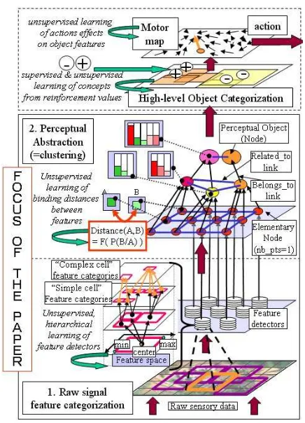
The global architecture of our epigenetic system can be roughly described as a superposition of self-organizing layers (fig.1). We first have a local feature detectors layer and an abstraction layer that together segment raw data into perceptual ”objects”. Then the percepts are orga-nized in higher level categories that may serve recog-nition. An affective layer evaluates the key-features of these higher-level categories which relate to the concepts of “good” and “bad” from reinforcement values. A mo-tor map layer that learns to relate elementary actions to
their effects on the concepts’ key features finally orients action.
2.
Paper focus
For a robot aiming at developing higher-level concepts about its environment, one fundamental problem is the abstraction of highly redundant sensory signals into a limited number of higher-level “objects” using a certain vocabulary of low-level features. This process is alter-natively called ”feature grouping”, ”perceptual organiza-tion”, ”saliency detection” or simply ”segmentaorganiza-tion”, and is the focus of the lower-level layers of our architecture.
While image segmentation has been intensively stud-ied most approaches make use of ad-hoc knowledge, whether they make hypotheses about the image, pre-define convenient features or set particular thresholds. Our goal here is to propose a biologically-inspired model of development for “perceptual organization” that avoids as much as possible ad-hoc settings through the use of unsupervised learning mechanisms.
Our argument will be articulated into two parts. We will first describe the development of low-level local fea-ture detectors that can perform a piecewise categorization of the input. The aim of this layer is to discretize a con-tinuous and complex input signal using a finite vocabu-lary (or “codebook”) of features. Then we will consider how these local features can be grouped using an agglom-erative clustering mechanism whose underlying similar-ity measures are learned from the features co-occurrence statistics. Using Information Theory we will define what a “good” abstraction level is and see how segmentation results are adapted to the robot’s experience. The mech-anisms we proposed will be illustrated with examples in both color and edge segmentation.
3.
Global design choices
Traditionally, the computational model of choice to emu-late biological processes are Neural Networks (NN). One problem with classical NN is that simply co-activating el-ementary symbols leads to binding ambiguity when more than one composite symbol is to be expressed; this is the “binding problem” [von der Malsburg, 1995] [Rosenblatt, In Berthouze, L., Kozima, H., Prince, C. G., Sandini, G., Stojanov, G., Metta, G., and Balkenius, C. (Eds.) Proceedings of the Fourth International Workshop on Epigenetic Robotics
1961]. In NN feed-forward hierarchies, the only way to capture increasingly complex features are combination or “grandmother” cells, which leads to combinatorial explo-sion. For the needs of compositionality, a mechanism of dynamical binding between neurons or group of neurons is needed [Bienenstock and Geman, 1995].
Basic bricks: We decided to use programming object-oriented concepts that are well-adapted to the recursive representation of abstraction hierarchies and the dynami-cal “binding” of distributed information. The basic brick of our system is a “Node”. Standing for an assembly of cells, it can bind the information from different feature spaces into one entity. A node may for example stand for a simple image pixel along with its features “posi-tion” and “color”, or for a whole object with features like “shape”, “position” or “motion”. Just like neural popu-lations may be composed of smaller ones, Nodes can be hierarchically linked using “belongs-to” and “contains” links. These links can code a conjunction of information as well as a change in the level of abstraction at which information is considered. “Related-to” links represent at one abstraction level the possible interactions between topologically neighboring Nodes. Each Node also has an identification and a level within the hierarchy. A global size variable gives the number of elemental particles con-tained (nb-pts) in a Node.
Information coding: Within each Node, information about a particular feature is considered statistically as a histogram over component features’ categories. This de-sign choice reflects the recent insight that information is coded in the brain by populations of broadly tuned neu-rons (“coarse coding”) in the shape of Probability Density Functions [Pouget et al., 2000] [Anderson and Van Essen, 1994]. As expressed by [John, 2001],”The activity of any individual cell is informational only insofar as it contributes to the overall statistics of the population of which it is a member”.
Basic processing and initialization: Within our framework, processing and learning will be seen in terms of object creation, updating and dynamic binding. Clus-ter analysis will be used as a unifying principle from low-level vision abstraction to higher-level categoriza-tion. The basic strategy of clustering is simple and gen-eral: according to a certain similarity principle (to be de-fined in section 5), some Nodes are grouped together and the resulting “group” Node summarizes information of interest in underlying Nodes’ attributes.
Before perceptual abstraction takes place, raw data is first filtered through the feature detectors. At each loca-tion a detector outputs for a local signal a histogram over its corresponding feature categories. These histograms will be the initial data of elementary Node (nb-pts=1) be-fore clustering starts. The initial topological neighbor-hood relationship between elementary Nodes (“related-to” links) is given.
Figure 1: The general architecture of our system. The lower layers of “feature categorization” and “perceptual abstraction” are the focus of the paper.
4.
The development of feature detectors
4.1
Biological process
In the visual cortex some neurons act in a very selective way as feature detectors within a certain physical ”recep-tive field” (e.g. selec”recep-tiveness to a bar of a certain orien-tation, color or form). Neurons responding to similar ori-entations are grouped in columns and such columns ag-gregate in ”hypercolumns” with all preferred values for common receptive field. A cortical map can thus carry out a complete piecewise analysis of the input in terms of “local features”. Cortical maps were found to self-organize according to the type of input and on the basis of experience [Hubel and Wiesel, 1962]. Our goal here is to emulate the development of such hypercolumns.
4.2
Mathematical models
not biologically plausible (only outputs are), they need pre-processing (e.g. whitening) and take a long time to converge. We experimented with Hyvarinen fast method [Hyvarinen and Hoyer, 2001] but found the setting of pa-rameters difficult and had stability problems within our dynamic environment. Another problem was the non-hierarchical shape of obtained codebooks: it is compu-tationally very heavy to compare each single input with all basis vectors.
The key concept of recoding the sensory signal through a codebook of feature detectors is the preservation of formation using as little structure as possible. For in-stance, for an input signal characterized by a certain prob-ability distribution, it is more interesting for a feature de-tector neuron to be selective for inputs around peaks of distribution than in a range that has few chances to occur. This is the reason why Infomax methods like Independent Component Analysis try to find the peaks of distribution for a random signal. We thought this behavior could be approximated by simpler winner-takes-all categorization methods1, and decided to take inspiration from Carpen-ter and Grossberg’s (Fuzzy) Adaptive Resonance Theory (ART) [Carpenter et al., 1991] that was introduced as a theory of human cognitive information processing and is well known for its fast and stable learning capabilities.
The main feature of ART systems is a matching process between bottom-up input vector and top-down learned categories. This matching leads to a ”resonant state” that triggers prototype learning if the input vector is close enough to the stored pattern or -if matching does not occur within a certain tolerance (”vigilance”)- cre-ation of a new pattern similar to the input vector. That no stored pattern is modified unless it matches the input vec-tor within a certain tolerance means that the system has both plasticity and stability.
4.3
Basic architecture description
Our system goal is to progressively develop feature de-tectors, neurons with a certain selectivity in feature space, that will recode an input signal. This development is pro-gressive and hierarchical and follows the shape of the probability distribution of the signal towards its peaks. One basic feature detector cell is represented by a Node.
Category representation. Each feature detector Node has a certain selectivity, corresponding to a certain cat-egory of signal feature. We express this catcat-egory as a hyper-rectangle in data space, with a ”range” defined by a minimum and a maximum in each dimension (min[i], max[i]) (fig.1). Each category also includes variance of
1Infomax models like ICA consider a signal S is represented as a linear superposition of a set of basis functions Ai: S=∑isi.Ai
(gen-erative approach). Learning rules could be generalized as a distri-bution density gradient-following process similar to competitive cate-gorization methods: Anew
i ←Aoldi +f(xTAiold)(x−Aoldi )with f(x)∈
[0,1]associated with decorrelation of basis vectors: Ap+1=Ap+1−
α∑j∈[0,p]ATp+1Aj.Ajand re-normalization Ai=|AAi|.
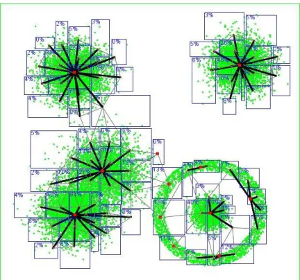
Figure 2: Category learning with 2D data points (in green). Cat-egories are rectangles (in blue). Neighborhood links are thin lines (in gray). Complex cells are thick points (in red) and links to simple cells are thick lines (in black). Down-left we can no-tice two mixed gaussians had their peaks correctly detected
data for each dimension (var[i]) and keeps in memory the total number “nb” of points it contains, that is to say the number of input vectors that entered in resonance with it.
Category updates and creation. Similarly to ART, there is a matching process between bottom-up input vec-tors X and top-down learned categories C. To evaluate a matching, the measures of similarity between two vectors X and Y we use are:<x,y>=1−( 1
dim.∑i(x[i]−y[i])2)−
1 2and<
x,y>= X.Y
|X|.|Y| (dot product). Similarity between a vector X
and a category C is in both cases<X,C>=miny∈C<X,y>.
If the matching value is below a certain vigilance, a new Node with a new category is created with :
max[i] =min[i] =center[i]
var[i] =0 nb=1
Otherwise there is resonance and the Node of closest category is updated as:
i f(x[i]>max[i])max[i] =U(nb)∗x[i] + (1−U(nb))max[i]
i f(x[i]<min[i])min[i] =U(nb)∗x[i] + (1−U(nb))min[i]
var[i] = (nb∗var[i] + (x[i]−center[i])2)/(nb+1) center[i] =V(nb)∗x[i] + (1−V(nb))∗center[i]
nb+ +
U and V are 2 parameter functions that determine the rate of adaptation of the borders and the center of a cate-gory.
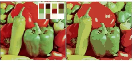
inter-Figure 3: Category learning results as color quantization: an in-put signal can be recoded using a vocabulary of 11 colors with-out an important loss of information
section is easy to test: if∃i/(minA[i]>maxB[i])∪(maxA[i]<
minB[i])then the two categories do not intersect.
A hierarchical process. We embedded this basic learning scheme in a hierarchical architecture where each Node can recursively point to sub-category Nodes start-ing from one “Root” which range is the whole feature space ([m[i], M[i]). The process of matching and updat-ing categories is recursively done at each level of the hi-erarchy. The maximum number of subnodes a node can have is defined beforehand.
Using the number of points “nb” in a category, the sys-tem can recursively maintain for each category an esti-mation of its importance, that is to say the probability for a future input vector to enter in resonance with it:
Proba=E( nb
nb−root)with“nb-root”the total number of vectors
that entered the root Node.
Using these statistics, a category can split in subcate-gories when it reaches a certain probability(Proba>Pmin), at the condition its variance, volume and size are im-portant enough. ”Splitting” may inititiate uncommitted (nb=0) subcategories randomly or according to the high-est variance direction. Inversely, categories of negligible importance can be deleted at periodic checks. A parallel can be drawn with the natural processes of growth and death of cells.
Neighborhood links. Every time a category is updated and grows, the system recursively checks if it comes in the neighborhood of another category, and in that case a “related-to” link is created between the two category nodes. for two categories A and B if ∃i/(minA[i]−maxB[i]
M[i]−m[i] >
α)∪(minB[i]−maxA[i]
M[i]−m[i] >α) then A and B are not neighbors. α
determines how close the categories A and B must be to be defined as neighbors. Ifα=0 the categories must be in contact. It is therefore possible to maintain for the low-est nodes of the hierarchy a knowledge of neighborhood relationships (2D “neighbors links” can be seen in fig.2).
Simple and complex cells. We call the lowest nodes of the hierarchy “simple cells”. Since it would be inef-ficient to account for different prototypes whose centers
converged to a similar peak of distribution, a final one-step clustering method links each “simple cell” Node to a “complex cell” Node. The procedure is the follow-ing: Each node can be given a ”density” corresponding to Proba
vol=∏i(max[i]−min[i]) from its probability and its volume in feature space. Starting from the densest, for each simple cell we check among its neighbors of higher density the closest Node N2, and if the similarity between N1 and N2’s attractor is higher than a threshold then N2’s attrac-tor becomes also N1’s and is updated accordingly; else a new attractor is created with N1 values. The ”complex cells” thus obtained may not correspond exactly to the bi-ological elements, but they do present a more complex se-lectivity by pooling ”simple cells”. Complex cells are au-tomaticaly listed and each obtains an identification num-ber aid∈[0,NBC]with NBC the total number of complex
cells.
Utilization. The recursive search for an input vector’s category can be very efficient in the case we limited the number of subnodes to two and used the non-overlapping mode, since at each level we just need to check if input x is within the range of one category. Though within a feature space not fully explored that may lead for some inputs to suboptimal classification, this has never been a problem in practical use.
4.4
Results
The “parameter functions” we used areU(x) =1: any new
vector is absorbed within the range of the category and
V(x) = 1
nbso the center of a category converges to the data’s
mean.
The behavior of the algorithm in 2D is illustrated in fig.2 with a data distribution of 10,000 points. With a high vigilance (0.93), the system developed a high num-ber of ”simple cell” categories that were then clustered in ”complex cells”. Categorization was immediate.
In the case of color information, our method showed to be an efficient color quantization algorithm. Fig.3 shows the famous ”pepper” image expressed with a codebook of 11 categories. Learning was immediate.
We also applied our algorithm to the categorization of local shape features. To express the local shape of a luminance signal x[i], all input X are re-centered so that ∑ixi=0, then inserted in the system using the dot
product similarity measure. In that example, we used
V(x) =<x,Ai.center>3to imitate Infomax methods’ learning
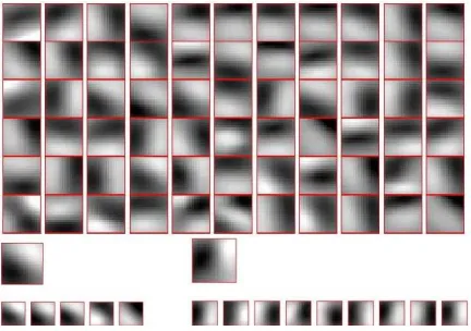
rule. Fig.4 shows a feature codebook that was learned in 3 to 4 minutes of exploration for an image definition of 200*200 and patches of 15*15. The figure under it shows the example of one ”complex cell” with related ”simple cells”. Learned detectors present an orientation selectiv-ity with differences in shift like their biological models.
Figure 4: Learned codebook of localshape feature detectors (15*15). Down: two examples of complex cell and associated simple cells
5.
The development of perceptual binding
5.1
Biological process
The following question is that of ”perceptual grouping” or ”object unity”: how locally coded representation of features can be ”gathered” together into a holistic per-ception? In the first half of the century, the gestalt school tried to explain perceptual organization by certain sim-ple ”laws” like grouping by proximity, similarity, clo-sure, symmetry, and good continuation [Koffka, 1935], but the underlying neuronal processes were largely un-known. It was then experimentally found that neurons in separated columns of the visual cortex are able to syn-chronize their oscillatory spiking-activities. This lead to the proposal that ”perceptual binding” might be per-formed by the visual cortex organizing into separate neu-ron groups defined by synchneu-ronization [Gray and Singer, 1987] [von der Malsburg, 1995]. The degree of synchro-nization would represent the perceptual saliency of an ob-ject. Evidence supports the idea that this synchronization could also subserve the integration of memory, emotions, motor planning [Varela, 1995]. The ability to achieve object unity seem to not be fully-formed in the neonate but to develop over time [Johnson, 2002] and it had been shown that synchronizing connections are susceptible to use-dependent modifications [Herculano and al., 1999].
5.2
Mathematical interpretation of binding
As stated previously, an important concept is the Bar-lowian principle of “redundancy reduction” [Barlow, 1961]: the goal of a perceptual system should be to min-imize statistical dependencies of its inputs and come up with a compact and sparse code. Asking what kind of in-formation would be worth noting and keeping for a per-ceptual system, Barlow advocated the concept of ”suspi-cious coincidences”: the co-occurence of two events A and B may justify remembering if this co-occurence is surprising (=unlikely) given prior knowledge of the
oc-curence of individual events. Inversely two components A and B should be combined in a composite object if they can “predict” each other, since it may be a waste of resources to consider them independently. An equiv-alent view of the problem, that fits well our framework, would be to see clustering as the transmission of maxi-mum information using as few components -or Nodes- as possible.
5.3
Learning a similarity measure.
To progressively cluster local features, we need a similar-ity measure. However, in our system, a similarsimilar-ity mea-sure between two input vectors A and B is not based on a pre-defined distance (e.g. cartesian distance), but de-pends on their statistical co-ocurrence. This learning is possible because of the discretization of the input signal in a finite number of feature categories.
The procedure is the following: at each time step, for N elementary Nodes randomly chosen, the system con-siders all direct neighbor nodes. The relative position of two nodes can be classified according to AO angular ori-entations and thus coded by a number d∈[0,AO]. Since each elementary Node refers to one of the NBC “com-plex cell” feature categories that was learned during the first phase, a feature A can be coded by its identification number a∈[0,NBC].
With such a code, it is possible to keep a statistical ta-ble of co-ocurrences T[AO][NBC][NBC] by increment-ing, every time a couple of features (A,B) of identifica-tion number (a,b) with direcidentifica-tion d∈[0,AO]is randomly registered, the elements T[d][a][b], T[d][b][a], T[d][a][NBC], T[d][b][NBC] and Total; where Total is the total number of observed Node couples andT[d][a][NBC] =∑iT[d][a][i].
The probabilities of the different events can be writ-ten: P(B) =T[d][b][NBC]
Total and P(B/A,D) = T[d][a][b]
T[d][a][NBC]. A possible
coefficient of “Suspicious Coincidence” between two el-ementary nodes (A,B,D) can therefore be written:
SC(D,A,B) =P(B/A,D)
P(B) =
Total.T[d][a][b]
T[d][a][NBC].T[d][b][NBC]
The logarithm of this measure can also be used: this is the Mutual InformationSC(D,A,B) =log(P(A,B,D)
P(A)P(B))of events
A and B. With such a measure, grouping can be seen as a result of a minimum mutual information partitioning, that is also a form of sparse coding.
However, since such measure may be difficult to in-terpret without re-normalization, we use in practice (and with better results!)- another measure of “suspicious co-incidence” that is symmetric and in the range [0,1]. If we writeT[d][a][max] =maxbT[d][a][b], the measure we propose
is :SC(D,A,B) = T[d][a][b]+T[d][b][a]
T[d][a][max]+T[d][b][max] which is equal to 1 for a
couple (A,B) if they are both the most common neighbor of the other.
Extension of the measure to feature histograms.
refer-ing to an histogram of activity over feature categories. If we write the histogram data S of a non-basic Node:
S=∑isi∗Ai
∑isi , the similarity measure of a couple of Nodes of histograms K and L is:SC(D,K,L) =∑i,jki∗ljSC(D,Ai,Aj)
∑iki∗∑jlj
Segmentation strategy. Once percepts have been fil-tered and represented within “local feature” Nodes, the progressive ”binding” of these Node will be realized in our system by a classical bottom-up greedy clustering. Nodes that synchronize together shall point to a similar superior Node that abstracts the information detained by underlying Nodes through a weighted fusion of their his-tograms (using nb-pts).
Neighbor relationships (“related-to” links) that also represent possible synchronizations, are given for the lowest nodes right at the output of the feature detectors, and then propagated according to the Nodes’ fusions.
Since the creation of new Node objects for each new segmentation would be very computationally heavy, all nodes are in fact already instantiated in one big table. What we do is therefore only to dynamically update pointers and contained data while keeping for each level of abstraction the indices of starting and ending node in the table. Our clustering algorithm is the following:
Given a threshold T For each node N1 at level n
. Check the most similar neighbor N2 . If(similarity>T)(
. If N2 has no superior Node give a sup. to N2 . Link N1 to N2’s superior and update the superior . )else set N1’s superior as a copy of itself Decrease threshold T
The only parameter of the algorithm is the pace at which the threshold T is decreased. A slower pace will give a little bit more robustness to the clustering at the expense of memory and speed. The choice of this pace is not critical though.
Stopping criterion. We do not use a stopping criterion but instead let the algorithm run until the whole visual scene can be summarized in one Node, we then backtrack to find an appropriate level of abstraction we characterize as preserving as much information as possible within as few Nodes as possible.
If we write I(Li,X)the mutual information between
the Nodes of the abstraction layer Li and raw input data
X; δIi=|I(Llast,X)−I(Li,X)| measures the gain in mutual
information when considering the level of abstraction
Li instead of the last level with the unique Node Llast.
Our criterion is to find the global maximum of the “per-tinence” function S(i) =|I(Llast,X)−I(Li,X)|
log(1+nb−nodesi) that evaluates the gain of information relatively to the number of Nodes used nb−nodesiwhen considering a percept at
abstrac-tion level Li.
δIi can also be written using conditional entropy as:
δIi=|H(Llast/X)−H(Li/X)|=|H(Llast/X)−∑iPi.H(Ci/X)|, where
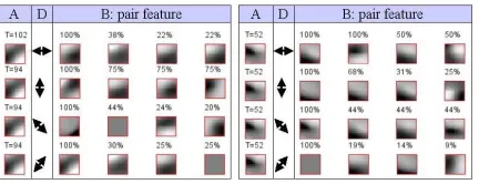
Figure 5: An example of learned table: for one feature (A) and one orientation (D), the most common features (B) are shown with their probability (normalized to the maximum). We can remark the self-similarity along the feature’s orientation.
H(Ci/X) is the conditional entropy of a cluster Ci
rela-tively to its raw input X and Pi is its proportional size
in the scene: nb−pts−Ci
nb−pts−Cf inal. During clustering, though in-formation on the pixels’ position is progressively lost, information on the other features is summarized in his-tograms. The conditional entropy of a cluster C con-taining the histogramK =∑ikiAi relatively to its raw
in-put X is thus equal to its conditional entropy with itself:
H(C/C) =∑i,jki.kj.log(P(Ai/Aj)). This measure could be
in-terpreted as a measure of the “stability” of the cluster C. The pertinence function S(i)has one global maximum that determines the level of abstraction at which the robot will consider its visual field. With our clustering method, based on a measure of similarity other than Mutual In-formation, S(i)may present several local maxima, corre-sponding to different numbers of clusters. As the robot moves in its environment, qualitative changes in decom-position can occur as a local maximum becomes global.
5.4
Results
We used our method to segment images using color and edge orientation. A ”Suspicious Coincidence” ta-ble was learned for image patches using four directions:
(0,π/4,π/2,3π/4)(fig.5) and in the case of color with no orientation distinction. The visual scenes presented to the system were synthetic images from a 3D simulator and pictures from a thematic series.
Feature segmentation was done using a coverage of 5*5 pixels patches in 200*200 images so that two neigh-bor basic nodes share half their receptive field. Our al-gorithm was able to segment simple simulator images into more or less ”homogeneous” and ”line” areas (fig.7). However no contour completion can be done with our al-gorithm since local relationships of features are progres-sively lost while homogeneous clusters emerge. Real-world images were less successful and will need further enquiry.
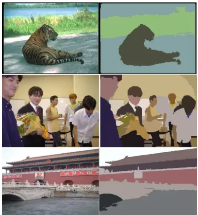
Figure 6: Color segmentation of real-world images from the-matic series.
white and black squares composing the wall should be seen as one entity (fig.8).
The stopping criterion had been tested with both simu-lator and real images and produced results, on the choice of a level of abstraction, that were coherent with the choice a human user would have done. Within the simu-lator, the criterion also proved to be robust, with a good stability in the decomposition of a scene from one frame to the next. Changes in abstraction level happen for in-stance when the robot moves towards an object until this object occupy most of the field of vision; details of this object then “spring out” (fig.8).
Segmentation times on a Pentium IV 2.5Ghz were typ-ically less than 0.3 seconds for a 200*200 image in 8-10 abstraction steps. The code is in Java.
6.
Conclusion and future work
With “traditional” segmentation techniques, one has to choose between robustness and speed. The simplest method such as thresholding can be used in real-time applications but face problems with more complex tex-tured images. On the other hand, global energy opti-mization methods can perform quality segmentation but are computationally heavy. A common weakness is a reliance on ad-hoc parameters. (For a review see [Pal and Pal, 1993].) Adaptive approaches were proposed, but they usually rely on a pre-specified evaluation function [Bhanu and Lee, 1994] or a database of manually seg-mented images [Meila and Shi, 2000]. Fewer approaches have the goal of biological modeling, e.g. oscillatory net-works [Terman and Wang, 1995]; but these are sensitive to noise.
We presented models of development for both lo-cal feature detectors and perceptual binding based on
Figure 7: Up: Edge grouping on simulator image. Down: Edge grouping with real-world images (“peppers” and “tiger” images shown previously in fig.6). A random color expresses a syn-chronized group of neurons.
neurobiologically-inspired dynamic mechanisms. While our method inherits the simplicity and speed of pixel clas-sification and clustering techniques, our system can au-tonomously learn from local statistics binding rules that may handle more complex patterns (e.g. textures). More-over, the learning of co-occurrence statistics between fea-tures allows an Information Theoretic interpretation of what a “pertinent” decomposition is. Another -more fundamental- result of this work is the demonstration that Perceptual Organization (and hence the Gestalt Criteria) could be based on minimal and generic bottom-up mech-anisms with a simple probabilistic foundation.
Thanks to segmentation, we now have the decomposi-tion of a scene in few high-level objects with statistical features (e.g. color histograms). These objects can be further characterized by their envelope’s shape and their position in the scene. From this level, we are now investi-gating how more complex features - like “object features” - can be developed in a bottom-up manner, and how they can be linked with the top-down reinforcement values that characterize a concept. Our strategy is to extend the simple and general idea of Adaptive Resonance Theory from vectors of fixed dimension, to non-dimensional en-tities like histograms, weighted combinations of features, and recursive compositions of objects.
References
Anderson, C. and Van Essen, D. (1994). Neurobiolog-ical computational systems. Computational
Intelli-gence Imitating Life. IEEE Press. 213-222.
Barlow, H. (1961). Possible principles underlying the transformations of sensory messages. Rosenblith, W.
A., editor, Sensory Communication, pp217-234.
Bell, A. and Sejnowski, T. (1997). The ’independent components’ of natural scenes are edge filters.
Vi-sion Research, 37:3327-3338.
Bhanu, B. and Lee, S. (1994). Genetic learning for adap-tive image segmentation. Boston MA Kluwer
Aca-demic Publisher.
Bienenstock, E. and Geman, S. (1995). Compositional-ity in neural systems. In Arbib, M. A. Editor,
223-226.
Carpenter, G., Grossberg, S., and Rosen, D. (1991). Fuzzy art: Fast stable learning and categorization of analog patterns by an adaptive resonance system.
Neural Networks, vol. 4, pp759-771.
Gibson, J. (1979). The ecological approach to visual perception. Houghton Mifflin. Boston MA.
Gray, C. M. and Singer, W. (1987). Stimulus-dependent neuronal oscillation in the cat visual cortex area 17.
IBRO Abstr. Neurosci. Lett. Suppl. 22.
Herculano and al. (1999). Precisely synchronized os-cillatory firing patterns require electroencephalo-graphic activation. J. Neurosci. 19, 3992-4010.
Hubel, D. and Wiesel, T. (1962). Receptive fields of single neurons in the cat’s striate cortex. J. Physiol.
148, 574-591.
Hyvarinen, A. and Hoyer, P. O. (2001). A two-layer sparse coding model learns simple and complex cell receptive fields and topography from natural images.
Vision Research, 41(18):2413-2423.
John, E. (2001). A field theory of consciousness.
Con-sciousness and Cognition 10, 184-213.
Johnson, S. (2002). Development of object perception.
Nadel and Goldstone (Eds.). Enc. of Cognitive Sci-ence, vol.3, pp392-399. Macmillan, London.
Koffka, K. (1935). Principles of gestalt psychology.
Harcourt, Brace and World, New york.
Meila, M. and Shi, J. (2000). A random walks view of spectral segmentation. Advances in Neural
Informa-tion Processing Systems. 873-879.
Olshausen, B. and Field, D. (1996). Emergence of simple-cell receptive field properties by learning a sparse code for natural images. Nature,
381:607-609.
Pal, N. and Pal, S. (1993). A review on image segmenta-tion techniques. Pattern recognisegmenta-tion, 26 1277-1294.
Pouget, A., Zemel, R., and Dayan, P. (2000). Informa-tion processing with populaInforma-tion codes. Nature
Re-view Neuroscience. 1(2):125-132.
Rosenblatt, F. (1961). Principles of neurodynamics: Perceptrons and the theory of brain mechanisms.
Spartan Books, Washington, D.C.
Terman, D. and Wang, D. (1995). Locally excitatory globally inhibitory oscillator networks. IEEE
Trans-actions on Neural Networks, 6. 283-286.
Varela, F. (1995). Resonant cell assemblies: a new approach to cognitive functions and neuronal syn-chrony. Biological Research 28, 81-95.
von der Malsburg (1995). Binding in models of percep-tion and brain funcpercep-tion. Current Opinion in
Neuro-biol. 5, 520-526.
Weng, J., McClelland, J., Pentland, A., Sporns, O., Stockman, I., Sur, M., and Thelen, E. (2000). Au-tonomous mental development by robots and ani-mals. Science, 291:599-600.