Stable Value Funds Performance
David F. Babbel
The Wharton School, University of Pennsylvania Miguel A. Herce
Charles River Associates
Abstract:
Little in the scholarly economics literature is directed specifically to the performance of sta-ble value funds, although they occupy a leading place among retirement investment vehicles. They are currently offered in more than one-third of all defined contribution plans in the USA, with more than $800 billion of assets under management. This paper rigorously ex-amines their performance throughout the entire period since their inception in 1973. We produce a composite index of stable value returns. We next conduct mean-variance analysis, Sharpe and Sortino ratio analysis, stochastic dominance analysis, and optimal multi-period portfolio composition analysis. Our evidence suggests that stable value funds dominate (on average) two major asset classes based on a historical analysis, and that they often occupy a significant position in optimized portfolios across a broad range of risk aversion levels. We discuss factors that contributed to stable value funds’ past performance and whether they can continue to perform well into the future. We also discuss considerations regarding whether or not to include stable value as an element in target date funds within defined contribution pension plans.
Key words: Stable value, defined contribution, optimal asset allocation, stochastic domi-nance
Stable Value Funds Performance
David F. Babbel*
Miguel A. Herce**
1. INTRODUCTION
In this updated study1 we reexamine the past history of stable value (SV) funds and their
per-formance over the past 43 years, with particular emphasis on the past 27 years. A growing volume of industry and practitioner research has provided a detailed look at how the funds are managed and stable values secured.2 Additionally, academic articles increasingly are
including SV funds within the purview of their studies,3 although it is difficult to find
in-depth scholarly treatments of SV funds performance outside of our preliminary working pa-pers.4 The lack of rigorous performance studies is rather surprising because SV funds
oc-cupy such a prominent place among retirement investment vehicles, with over $800 billion of assets under management.5 That puts them roughly on par with the increasingly popular
tar-get-date funds, which reportedly held some $880.4 billion of assets under management as of the end of 2016.6 SV funds are offered as an investment option in over one-third of all
* Professor Emeritus, The Wharton School, University of Pennsylvania. [email protected]
** Principal of Charles River Associates in Boston. [email protected]
This study was not supported nor sponsored by any organization or individuals. However, the authors express their gratitude to the Stable Value Investment Association (SVIA) for gathering the stable value return data used in this study, and to the Hueler Companies for providing us with their index of returns on stable value
commingled funds. The authors are fully responsible for their opinions and any errors in this study.
1 Our previous studies (Babbel and Herce, 2007, 2009, 2011) ended at the depths of the Great Recession and did
not include the most recent data from the past seven years.
2 See, for example, Stable Times, a quarterly publication of the Stable Value Investment Association, MetLife
Stable Value Study (2015), Paradis (2001), and Fabozzi (1998).
3 See, for example, Elton, Gruber and Blake (2007), Redding (2009), Tang et al (2009), and Gale et al (2016).
4 There is, however, a recent study in the professional actuarial literature that does broach on performance of SV
funds, although that it not its primary focus. Donahue (2016) reports some SV returns, volatilities and
correlations over the most recent 5, 10, and 15 years. He also provides useful information about varieties of SV fund structures. Additionally, customized performance benchmarks have been developed for SV funds. These measures incorporate client-specific factors in assessing the funds’ overall crediting rates. See Kruk et al (2012).
5The Stable Value Investment Association (SVIA) reported 164,913 member plans as of December 2015 and
members had $801 billion under management as of the second quarter of 2016. The SVIA has no current estimate on additional SV funds managed by nonmembers, but one estimate from 2010 pegged it at around $250 billion. In any case, the total assets managed in SV plans exceeds $800 billion and perhaps $1 trillion.
6 As reported in: “Is It Prudent for Investors to Use Target-Date Funds for Retirement Savings?” Wall Street
fined contribution (DC) plans, including 457, 403(b), 401(k) and some Section 529 Tuition Assistance Plans. By February 2009 they peaked at 36.7% of their assets due primarily to stock market declines, although allocations are more typically within the 10-25% range.7
More ironically, the lack of performance analyses did not forestall an onslaught of articles criticizing stable value and advocating that plan participants downsize their allocations to-ward the SV options.8
In this updated study, we provide a rigorous analysis of the performance of SV funds, enlist-ing an extended data set that goes from 1973 through 2015. We also include SV return data through the end of 2016 for informational purposes only.9 We compare their performance to
that of basic asset classes such as U.S. large and small stocks, long-term government and corporate bonds, intermediate-term government bonds, and money market funds, using three methods: mean-variance analysis, stochastic dominance analysis, and an enhanced multipe-riod utility analysis. Our study shows that since the inception of stable funds in late 1988, and their precursors in 1973, none of these other asset classes has dominated them; on the contrary, SV funds have dominated money market and intermediate-term government bond funds (and nearly dominated long-term corporate bonds as well) over a wide range of risk aversion levels and, when combined with small stocks and long-term government bonds, they occupy a prominent and often dominant part in optimal portfolios. 10
Before concluding our study we explain the value proposition for SV funds – how they have been able to generate notable returns for their investors – and whether the contributors to their past performance can be expected to continue into the future. We consider the recent financial crisis and revisit how the funds have weathered that crisis. We comment briefly on the themes and considerations of plan sponsors and their fiduciaries who choose not to in-clude SV funds in their menus of options for plan participants and consider complications for incorporating SV in the increasingly popular target date funds.
Act of 2006 (PPA), wherein the Department of Labor granted a safe harbor (from lawsuits) for plan sponsors who chose target date funds as the default investment choice for their employees, stable value funds accounted for about 60% of the assets in 401(k) plans that offered them as an investment option., according to VanDerhei, et al (2017). This dropped to only 49% by 2014. Moreover, the percentage of plans including SV among its investment alternatives dropped from 51% in 2006 to 35% in 2014. Notwithstanding these legislative initiatives, SV’s popularity in terms of assets under management continues to keep pace with target date funds.
https://www.stablevalue.org/index.php/news/article/stable-value-assets-continue-to-grow
7 According to EBRI (2017), older participants in their 60s hold about 20% of their assets in SV, whereas
younger participants in their 20s typically allocate less than 5% to SV (see chart 23).
https://www.ebri.org/pdf/briefspdf/EBRI_IB_436_K-update.3Aug17.pdf Current statistics are available at
www.stablevalue.org
8 See GAO (2011).
9 We do not incorporate these 2016 data in our performance analyses because the SBBI data series for two of
our alternative asset classes is not being maintained after 2015, and we did not wish to introduce a statistical discontinuity by piecing together alternative sources with divergent survey protocols as proxies for the original data series for a gain of only a single year.
10 They also dominated even more strongly the returns exhibited on the SBBI mixed index of intermediate
2. BACKGROUND
Stable value funds are labeled in various ways, including Capital Accumulation, Principal Protection, Guaranteed, Preservation, Income funds, as well as Guaranteed Investment Con-tracts (GICs) and Group Annuity ConCon-tracts, among others. Early forms of SV funds have been around since the 1970s, coinciding with the development of U.S. defined contribution (DC) plans. From their outset, these funds consisted largely of laddered maturity GICs11
issued by insurance companies. The returns, which were guaranteed regardless of the per-formance of the underlying assets, were fully backed by the GIC issuer’s general account. Over time, some plan sponsors sought an alternative structure that would provide them with greater flexibility and control, as the assets backing the GIC contracts were owned and man-aged by the insurer and the underlying investment strategy was that of the insurer’s general account.
Such concerns were addressed, in part, with the creation in late 1988 of separate account GICs, where the assets underlying the contracts, although still owned by the insurance com-pany, were held in separate accounts for the exclusive benefit of the plan(s) participating in the separate account and could not be used to discharge claims against the general account of the insurer. In this structure, the guarantees against any investment shortfalls stemming from poor performance of the separate account assets were still secured by assets in the general account and surplus. This innovation provided additional flexibility to fund managers, who could pursue a customized investment strategy rather than a general account investment strategy.
Then, in mid-1994, the SV funds market broadened when synthetic GICs (also called Trust GICs) were created in an effort to allow plans to retain legal title to plan assets, and to pro-vide additional flexibility in terms of investment strategy and asset selection. This structure enabled non-insurers to manage the plan assets, which are directly owned by the participating plan(s), while the financial protections were secured by banks, insurers, and other financial institutions. Today synthetic GICs occupy a prominent position in stable value, and coexist with traditional and separate account GICs.12 Each structure of stable value carries features
that are preferable to different plan sponsors. Some prefer the yields and generous plan ad-ministration fee offsets that may be available through general account GIC-based plans; oth-ers prefer the investment flexibility of separate account GICs, while still othoth-ers seek the un-derlying asset ownership feature of synthetic GIC-based funds.
A stable value fund offers principal protection and liquidity to individual investors, and steady returns that are roughly comparable to intermediate-term bond yields, but do not ex-hibit the volatility of intermediate-term bond total rates of return. Additionally, over ensuing one-to-six-month intervals (depending on the SV contract), the guaranteed rate of return moves more slowly than intermediate-term bond yields. This is achieved by having a pro-cess and investment contract, discussed in the following section, that allow the provider to
11 Traditional GICs are issued by an insurance company that guarantees the principal invested and pays a
periodically-reset interest rate for a certain period of time.
smooth market volatility through amortizing gains and losses over the duration of the portfo-lio. This smoothing is effected through crediting rate reset mechanisms and protocols that insulate investors against day-to-day volatility. As a consequence of these features and the underlying short to intermediate-term fixed income investments, SV funds provide investors with positive returns of very low volatility. This combination of bond-yield-like returns and low volatility obtains contract or book value accounting of the investment.13
The underlying investment portfolios of all three forms of stable value funds typically com-prise high quality, short maturity (usually under seven years) corporate and government bonds, mortgage-backed securities, asset-backed securities, and other structured products. In the case of synthetics, the portfolio is protected against interest rate risk through an invest-ment contract or “wrap” obtained from a high quality bank, insurer or other financial institu-tion. This means that in all but a few prespecified circumstances, investors in an SV fund are able to transact (make deposits, withdrawals, transfers) at book or contract value, which is deposits plus accrued interest, less any past withdrawals. In financial industry jargon, this is known as “benefit responsiveness.”
Stable value funds do not require a set holding period but provide participants full access to their principal and accumulated interest without a penalty. However, they are subject to gen-eral restrictions within the ovgen-erall plan. For example, many plans restrict participants from the direct transfer to a competing short-duration bond or money market fund by requiring that money transferred out of SV first be invested in a non-competing (e.g., stock or long-term bond) fund for a short period such as 30-90 days to eliminate arbitrage trading. This rule, together with the fact that plan participants do not act in concert regarding the allocation of their funds, allow the investment contract protections (“wrappers”) to be purchased for a fraction of what it would cost if interest arbitrageurs pervaded the pool and were revising their allocations aggressively.
3. CREDITING RATE FORMULA
From an investor’s viewpoint, SV funds operate somewhat like a passbook savings account. They accrue interest at a prespecified crediting rate that is generally updated periodically (every one to six months, in accordance with investment contract specifications) to incorpo-rate changing market conditions. Their principal is secure and grows over time by the amounts of interest credited to their account. Crediting rates on SV funds change more slowly than bond yields and may be guided according to a formula which basically produces an internal rate of return for the investment by requiring that the contract (or book) value of the portfolio converge to its market value by the end of the assumed duration. We define the variables in the formula as follows:
CR: crediting rate applied to the accounts of investors in the SV funds MV: market value of the underlying portfolio
CV: contract value of the underlying portfolio
D: duration of the underlying portfolio or duration of a benchmark portfolio
Y: yield of the underlying portfolio, as described further below. Given these variables, the future market value (FMV) of the portfolio is given by
= (1 + ) . (1)
The crediting rate that guarantees this value, given the current contract value, is the solution to
= (1 + ) . (2)
Therefore, the crediting rate formula is given by equating the right-hand-side of expressions (1) and (2), and solving for CR,
= (1 + ) − 1. (3)
Although other variations of the crediting rate formula are also used for guidance, expression (3) is the one most generally used.14 In addition to small differences in the crediting rate
formulae, managers do not always calculate the inputs to the formulae in the same way. For example, with respect to the measure of duration D, some fund managers use the duration of a benchmark portfolio, while others use the duration of the underlying securities. The yield measure Y is most often a duration market-weighted bond equivalent yield, although some variations have occurred.
Illustration 1 details how the crediting rate guiding formula is designed to make the contract value of the portfolio converge to its market value over the duration of the portfolio, assum-ing market conditions do not change in the interim. The case illustrated is where the contract value exceeds the market value, but the same procedure is used in the opposite case.
As indicated below, the crediting rate effectively smooths returns by distributing gains and losses over a period of time related to the duration of the portfolio. The crediting rate for-mula below implies that the crediting rate is between the portfolio’s return and its yield, Y, and closer to the portfolio’s yield the longer the duration, D, is. The important thing to re-member is that individual investors receive the same rate of return as the stated crediting rate, since principal is protected.
While this or a similar formula may serve as a starting point for a number of providers, ulti-mately (unless contractually specified otherwise) the crediting rates are determined by the provider itself, sometimes through committee decisions, and announced at or before the start of an ensuing crediting rate time interval. Furthermore, the crediting rates are set with com-petition in mind and a host of other economic factors. Investors are able to withdraw and redeploy their funds if they are dissatisfied with the pre-announced crediting rate, subject to the aforementioned restrictions.
4. PERFORMANCE MEASUREMENT
In this study we will measure the performance of SV funds vis-à-vis money market instru-ments,15 intermediate-term government bonds, long-term government bonds, corporate
bonds, and small and large stocks using three methods of analysis: mean-variance analysis, stochastic dominance analysis, and enhanced multiperiod utility analysis. Each method has its advantages and drawbacks, but together we get a fairly clear picture of how well SV funds have performed. We conduct our analyses over the 27-year period beginning in 1989 when separate account GICs became an important component in the stable value market and, as a robustness test, over the extended 43-year period starting in 1973 that was dominated early by general account GICs.
15 In our earlier studies, we used money market funds, but with the near disappearance of such funds post the
Great Recession, we switched to T-bills in this study. The results of those studies were very similar to what we observed in the present study.
Illustration 1: Setting Synthetic GIC Crediting Rates
Step 1
Calculate estimated future market value by compounding the current market value at the portfolio’s current yield to maturity for a period equal to the portfolio’s duration.
Source: SVIA
Step 2
Determine new crediting rate as the discount rate that equates the estimated future market value with the current contract value.
CV = $100
FMV = $111.36
MV = $99
Duration (D) = 3 years MV/CV = 99%
Future Market Value Contract value reflects net
deposits plus accrued interest
Market value reflects underlying portfolio’s actual market return
Step 2 Crediting rate (CR) = 3.65%
We begin with a mean-variance analysis, more because of its simplicity and ubiquitous use in practice than its theoretical properties.16 Strictly speaking, the validity of this approach
hinges upon whether investors consider variance to be an adequate measure of investment risk. In other words, investor preferences must be satisfactorily modeled using quadratic utility.
Beginning as early as 1967, Arditti determined that investors considered measures of down-side risk beyond variance, and countless additional studies along similar lines have continued until now to demonstrate that variance is an inadequate measure of either security or portfolio risk.17 However, if the distribution of market returns can be fully described by its first two
moments, then restricting one’s performance analysis to a mean-variance analysis can be justified, even if investors would otherwise be concerned about higher (and non-existent) moments of the return distribution. But all tests with which we are familiar demonstrate that return distributions for stocks, bonds, and money market instruments cannot adequately be characterized by their means and variances, nor does modified Brownian motion fully cap-ture the movement in these asset returns.
Accordingly, we next measure investment performance using stochastic dominance analysis. Introduced in 1969 by Hanoch and Levy and by Hadar and Russell to remedy certain short-comings of mean-variance analysis, stochastic dominance approaches have the clear ad-vantage of taking into account all moments and other characteristics of the return distribu-tions, and providing investment dominance analyses that do not depend upon knowing the exact shapes of investor preference functions. This has another distinct advantage over the mean-variance approach, which cannot be valid for various horizons simultaneously because it relies on log-normally distributed returns, and which if valid (under certain conditions) for single-period returns is not valid for multiperiod returns. By contrast, the stochastic domi-nance approach remains valid because it is distribution-free. The important additional virtues and limitations of this approach are discussed at length in the authoritative treatise by Levy (2006). While some of the limitations have been overcome by a plethora of research, dating from the 1970s to the present, there remain two:
1) Stochastic dominance methods do not provide guidance into the construction of a portfolio from various individual securities.
2) Stochastic dominance methods do not provide an equilibrium price for securities. Our third approach is an indirect approach to performance measurement, based on the dis-crete-time multiperiod investment theory of (1968), Hakansson (1971, 1974), Leland (1972), Ross (1974), and Huberman and Ross (1983). Sometimes dubbed Turnpike Portfolio The-ory, it remedies certain failings of mean-variance analysis as well as the limitations of
16 An excellent treatise on this approach is provided by Markowitz (1987).
17Indeed, as reported by Douglas (1969), John Lintner’s initial cross sectional tests conducted in 1965 found
chastic dominance analysis at the high cost of specifying the form of the intertemporal pref-erence function. To mitigate this high cost, in part, we will conduct our analysis across a wide range or risk aversion levels. Grauer and Hakansson (1982, 1985, 1986, 1987, 1993, and 1995) and others, applied this theory to the asset allocation problem with some success, where an empirical probability assessment approach was used to implement a set of invest-ment strategies. We will not rehearse the details of the methodology here, as they are well documented in Grauer and Hakansson (1986). The approach is indirect in the sense that we will determine whether, based on past asset return patterns and a range of current expecta-tions, SV assets would enter the optimal portfolio in any significant way.
5. DATA
The data of our primary focus are quarterly asset returns for the period Q4-1988 (shortly after the inception of stable value funds) through Q4-2015. We also include earlier data in Section 7 (Robustness Analysis), going back to Q2-1973, using the wrapped Lehman Intermediate Government/Credit Bond Yield series as a proxy for the return on traditional GICs, the pre-cursors of SV funds. In addition to stable value (SV) funds, we consider six other asset clas-ses, represented by large company stocks (LS), small company stocks SS), long-term corpo-rate bonds (LTCB), long-term government bonds (LTGB), intermediate term-government bonds (ITGB), and money market (MM). We describe each data series next.
Ibbotson’s stocks, bonds, bills, and inflation (SBBI) data are used for the following asset classes: LS (total return on the S&P 500), SS (the lowest 5% market cap in
NYSE/AMEX/NASDAQ, comprising approximately 1700 stocks), LTCB (Citigroup Long-Term High Grade Corporate Bond Index, with an approximate maturity of 20 years), LTGB (each year, a newly issued government bond with approximate maturity of 20 years is used to calculate total return), and ITGB (each year, a newly issued government bond with approxi-mate maturity of 5 years is used to calculate total return).
Money market returns are represented by the return on the Bank of America-Merrill Lynch US 3-Month Treasury bill Index (formerly the Lehman US Treasury Bellwether 3-Month Index). In Section 6.3, Intertemporal Optimization Analysis, where expected money market returns are an input to the optimization model, we use the yield series on 3-month Treasury bills, obtained from the Federal Reserve’s H15 database.
For SV funds, Q4-1988 – Q4-2015, we use total net quarterly returns on various SV fund families managed by members of the Stable Value Investment Association (SVIA.) From the stable value data we produce a composite index of stable value returns, including comingled funds, externally managed separate accounts, internally managed separate accounts, and life insurance general account stable value.18 As indicated above, when extending our analysis
18 Our stable value index (equal-weighted average of individual returns) is based on assets under management
of approximately $540 billion as of the end of 2015. Our composite index, which covered approximately 75,000 plans, included general account funds, externally managed separate account funds, and commingled funds. An alternative index available from Hueler Companies focuses on commingled funds. The Hueler Index is an equal-weighted total return average across all participating funds covered by Hueler and represents
back to the second quarter of 1973, we use the wrapped Lehman Intermediate Govern-ment/Credit Bond Yield series as a proxy for the return on traditional GICs during the period Q2-1973 – Q1-1988.
Although we have SV data for the four quarters of 2016, Morningstar stopped reporting the main SBBI series as of the end of 2015. It is mainly for this reason that our data end with the fourth quarter of 2015.
We note that except for small stocks and SV funds, reported returns are gross returns and need to be adjusted for management fees and transaction costs to be comparable to returns on small stocks and SV investments. We do this by subtracting average fees and expenses re-ported by the Investment Company Institute (ICI) for stock, bond and money market funds over the period of our analysis from the corresponding large stocks, bond or money market returns.19,20 Figure 1 below shows the evolution of mutual fund fees and expenses over the
period of our analysis.
sub-samples of externally managed separate account funds (which in aggregate constituted about 1/3 of all stable value funds). See http://www.hueler.com/ We found the Hueler index of commingled fund quarterly returns to be 99.8% correlated with quarterly returns on our equal-weighted composite index, and about 0.43 basis points apart per quarter, over the period Q1-1989 through Q4-2015.
19 Annual fund fees and expenses from 1980 through 1989 are from ICI’s Research Fundamentals, Vol. 14, No.
6, October 2005, pp. 3, 6, and 7. Annual fund fees and expenses from 1999 through 2015 were personally communicated to the authors by ICI. With regard to using the ICI’s fees and expenses numbers, their averages reflect both institutional and retail pricing and both kinds of funds are prevalent in plan sponsored retirement programs. However, using only institutional pricing would understate the full cost of intermediation, as discussed and summarized in an enlightening article citing several scholarly studies.
http://www.pattonfunds.com/pdf/The-Hidden-Costs-of-Mutual-Funds-WSJ-(00027720).PDF We regard the use of ICI’s numbers as a good compromise but in any case, as our study will show, the results are so overwhelming that they are unlikely to change appreciably by using only reported institutional pricing.
20 Stable Value crediting rates are net of contract and management fees through 2008. Due to changes in
Figure 1. Annual Fees and Expenses for Stock, Bond, and Money Market Funds
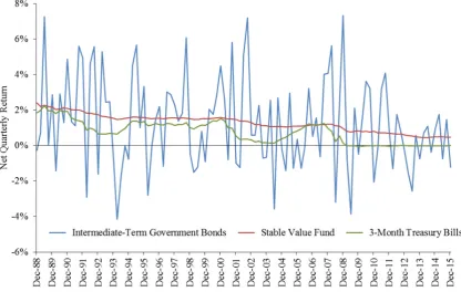
Using these data as well as asset values for each fund complex, we construct an equal-weighted average return series. Figure 2 plots this series together with net quarterly return series for the intermediate-term government bond fund and money market fund series.21
21 Early working papers created both equal-weighted and value-weighted average return indexes and our
Figure 2. Net Quarterly Returns – Stable Value Compared to ITGB and MM
Table 1 below presents summary statistics for the seven asset classes we study. It shows that over the period Q4-1988 through Q4-2015, SV investments have had, on average, a higher net quarterly return and a lower return volatility than either money market or intermediate-term government funds. As expected, when compared to stocks or long-intermediate-term bonds, SV funds have exhibited both lower average returns and volatility. These facts lie behind the results that we present in the next section.
Table 1. Summary Statistics – Net Quarterly Returns, Q4-1988 – Q4-2015
LS SS LTCB LTGB ITGB MM SV
Mean 2.41% 3.27% 1.84% 1.93% 1.24% 0.75% 1.28%
Median 2.71% 3.44% 1.64% 1.31% 0.99% 0.82% 1.37%
Maximum 20.97% 28.67% 23.18% 21.00% 7.33% 2.24% 2.40%
Minimum −22.18% −26.98% −12.61% −8.39% −4.15% −0.05% 0.44%
Std. Dev. 7.78% 11.03% 4.64% 5.41% 2.58% 0.63% 0.49%
Skewness -0.604 -0.250 0.638 0.671 0.326 N/A N/A
Kurtosis 0.721 0.260 3.886 1.235 -0.390 N/A N/A
Jarque-Bera 8.992 1.440 75.970 15.103 2.616 N/A N/A
6. RESULTS
6.1 Mean-variance analysis. As indicated earlier, mean-variance analysis
pro-vides a characterization of the trade-off between risk and return that is neither supported by the statistical properties of the return data, nor by the theoretical logic of risk aversion. De-spite these shortcomings, the mean-variance approach provides useful insights into the ability of SV investments to dominate other asset classes.
In this section we present evidence supporting the conclusion that, even as stand-alone vestment, SV funds have been superior in the mean-variance sense to money market and in-termediate-term government bond funds. We caution, however, that there are other im-portant aspects of performance, discussed later, which are not captured by mean-variance analysis, so one should not jump to conclusions about the dominance of SV funds over these other asset classes based solely on mean-variance analysis. We also show, based solely on historical returns, that when included in optimal mean-variance portfolios, SV funds contrib-ute significantly to the portfolio, to the exclusion of money market and intermediate-term government bonds, long-term corporate bonds and even large stocks. In other words, optimal mean-variance portfolios contain mostly SV funds, long-term government bonds and small stocks in proportions that naturally vary with the expected return (or, alternatively, the ex-pected volatility) of the optimal portfolio. We anticipate that in the future, allocations toward long-term government bonds would be less, given that their inclusion in optimal portfolios to date was augmented significantly by a protracted period of capital gains stemming from de-clining Treasury yields.
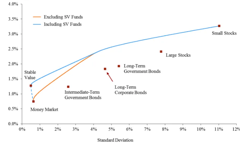
Figure 3. Efficient Frontiers for Alternative Asset Classes (Q4-1989 – Q4-2015)
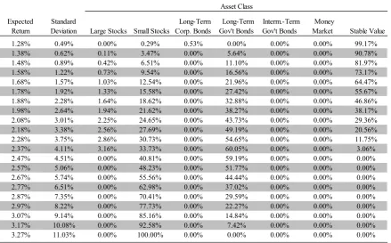
It is interesting to note the potentially large scope for improvement that inclusion of SV in-vestments brings to an optimal mean-variance portfolio across about half of the expected return range. As revealing as Figure 3 is, it does not show the full extent to which SV in-vestments contribute to an optimal portfolio since it says nothing about the relative alloca-tions of wealth among SV funds and other investments at different points along the efficient frontier. Table 2-A reports these optimal weights (again based solely on historical returns) for selected expected quarterly returns ranging from 1.28%, the historical average net return for SV funds, to 3.27%, the historical small stocks net return.
Table 2-A. Optimal Portfolio Weights for Mean-Variance Efficient Portfolios Including SV (Q4-1988 – Q4-2015)
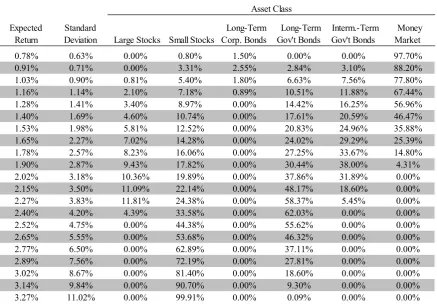
Table 2-B repeats the optimal portfolio analysis but where SV is not included as an available asset class. We observe that money market instruments and intermediate-term bonds now enter the optimal portfolios at various levels of portfolio risk, along with small and large stocks and term government bonds. We also observe that large US stocks and long-term corporate bonds modestly increase their presence among efficient frontier portfolios.
Expected Return
Standard
Deviation Large Stocks Small Stocks
Long-Term Corp. Bonds
Long-Term Gov't Bonds
Interm.-Term Gov't Bonds
Money
Market Stable Value
1.28% 0.49% 0.00% 0.29% 0.53% 0.00% 0.00% 0.00% 99.17%
1.38% 0.62% 0.11% 3.47% 0.00% 5.64% 0.00% 0.00% 90.78%
1.48% 0.89% 0.42% 6.51% 0.00% 11.10% 0.00% 0.00% 81.97%
1.58% 1.22% 0.73% 9.54% 0.00% 16.56% 0.00% 0.00% 73.17%
1.68% 1.57% 1.03% 12.54% 0.00% 21.96% 0.00% 0.00% 64.47%
1.78% 1.92% 1.33% 15.58% 0.00% 27.42% 0.00% 0.00% 55.67%
1.88% 2.28% 1.64% 18.62% 0.00% 32.88% 0.00% 0.00% 46.86%
1.98% 2.64% 1.94% 21.62% 0.00% 38.27% 0.00% 0.00% 38.17%
2.08% 3.01% 2.25% 24.65% 0.00% 43.73% 0.00% 0.00% 29.36%
2.18% 3.38% 2.56% 27.69% 0.00% 49.19% 0.00% 0.00% 20.56%
2.28% 3.75% 2.86% 30.73% 0.00% 54.65% 0.00% 0.00% 11.75%
2.37% 4.11% 3.16% 33.73% 0.00% 60.05% 0.00% 0.00% 3.06%
2.47% 4.51% 0.00% 40.81% 0.00% 59.19% 0.00% 0.00% 0.00%
2.57% 5.06% 0.00% 48.23% 0.00% 51.77% 0.00% 0.00% 0.00%
2.67% 5.74% 0.00% 55.56% 0.00% 44.44% 0.00% 0.00% 0.00%
2.77% 6.51% 0.00% 62.98% 0.00% 37.02% 0.00% 0.00% 0.00%
2.87% 7.35% 0.00% 70.41% 0.00% 29.59% 0.00% 0.00% 0.00%
2.97% 8.22% 0.00% 77.73% 0.00% 22.27% 0.00% 0.00% 0.00%
3.07% 9.14% 0.00% 85.16% 0.00% 14.84% 0.00% 0.00% 0.00%
3.17% 10.08% 0.00% 92.58% 0.00% 7.42% 0.00% 0.00% 0.00%
3.27% 11.03% 0.00% 100.00% 0.00% 0.00% 0.00% 0.00% 0.00%
Note: Weights may not add up to 100% across a given row due to rounding.
Table 2-B. Optimal Portfolio Weights for Mean-Variance Efficient Portfolios Excluding SV (Q4-1988 – Q4-2015)
Continuing in the spirit of mean-variance analysis, we turn to the Sharpe ratio so commonly used in asset allocation and performance measurement.22 The Sharpe ratio measures excess
return per unit of risk according to the formula:
(4)
where R is the asset return, Rf is the return on the risk-free rate of return, and is the
expected value of the excess of the asset return over the risk-free rate. This ratio is used as a measure of how well an investor is compensated per unit of risk taken. Higher ratios denote greater return for the same level of risk.
We also use the Sortino ratio to focus more on the downside risk.23 The Sortino ratio is
based on the Sharpe ratio, but penalizes for only those returns that fall below the target
22 The original “Reward-to-Variability” performance ratio, better known as simply the “Sharpe ratio” of
William Sharpe was modified by him in 1994. The modified version of his ratio is used in this analysis. See Sharpe (1994).
23 See Sortino and Price (1994) and Sortino and Van der Meer (1991) for a description of the Sortino Ratio. The
theoretical foundations for the Sortino Ratio are provided in Pedersen and Satchell (2004).
Expected Return
Standard
Deviation Large Stocks Small Stocks
Long-Term Corp. Bonds Long-Term Gov't Bonds Interm.-Term Gov't Bonds Money Market 0.78% 0.63% 0.00% 0.80% 1.50% 0.00% 0.00% 97.70% 0.91% 0.71% 0.00% 3.31% 2.55% 2.84% 3.10% 88.20% 1.03% 0.90% 0.81% 5.40% 1.80% 6.63% 7.56% 77.80% 1.16% 1.14% 2.10% 7.18% 0.89% 10.51% 11.88% 67.44% 1.28% 1.41% 3.40% 8.97% 0.00% 14.42% 16.25% 56.96% 1.40% 1.69% 4.60% 10.74% 0.00% 17.61% 20.59% 46.47% 1.53% 1.98% 5.81% 12.52% 0.00% 20.83% 24.96% 35.88% 1.65% 2.27% 7.02% 14.28% 0.00% 24.02% 29.29% 25.39% 1.78% 2.57% 8.23% 16.06% 0.00% 27.25% 33.67% 14.80% 1.90% 2.87% 9.43% 17.82% 0.00% 30.44% 38.00% 4.31% 2.02% 3.18% 10.36% 19.89% 0.00% 37.86% 31.89% 0.00% 2.15% 3.50% 11.09% 22.14% 0.00% 48.17% 18.60% 0.00% 2.27% 3.83% 11.81% 24.38% 0.00% 58.37% 5.45% 0.00% 2.40% 4.20% 4.39% 33.58% 0.00% 62.03% 0.00% 0.00% 2.52% 4.75% 0.00% 44.38% 0.00% 55.62% 0.00% 0.00% 2.65% 5.55% 0.00% 53.68% 0.00% 46.32% 0.00% 0.00% 2.77% 6.50% 0.00% 62.89% 0.00% 37.11% 0.00% 0.00% 2.89% 7.56% 0.00% 72.19% 0.00% 27.81% 0.00% 0.00% 3.02% 8.67% 0.00% 81.40% 0.00% 18.60% 0.00% 0.00% 3.14% 9.84% 0.00% 90.70% 0.00% 9.30% 0.00% 0.00% 3.27% 11.02% 0.00% 99.91% 0.00% 0.09% 0.00% 0.00%
Note: Weights may not add up to 100% across a given row due to rounding.
Asset Class , ] [ ] [ Ratio Sharpe f f R R Var R R E − − = ] [R Rf
turn, which in our case will be the average riskless rate of return over the period of analysis. The ratio gives the actual rate of return in excess of the risk-free rate per unit of downside risk, and is as calculated below:
(5)
The Sharpe and Sortino ratios for quarterly net return data are reported in Table 3-A. Table 3-A. Sharpe and Sortino Ratios (Quarterly Data, Q4-1988 – Q4-2015)
Note: The target rate for the Sortino ratio is the average money market fund rate. Therefore, the numerator is the same in both the Sharpe and the Sortino ratios.
We note that the Sharpe ratio values for the non-SV asset classes are mostly clustered to-gether, but that for SV the ratio is more than seven times greater than the highest of the other asset classes. This pattern is even more pronounced for the Sortino ratio. The extremely high Sortino ratio assigned to SV funds, relative to those assigned to other asset classes, re-sults from the fact that throughout the entire 109 quarter period under consideration, the risk-free rate exceeded the SV credited rate only for four quarters (in Q3-2006 and Q1-Q3, 2007) and by small amounts. Hence, there were only a few, small observations that factored into the denominator.
What is most noteworthy about these performance ratios is how much higher they are for SV funds than for the other asset classes. Although our calculations are based primarily on quarterly data, we also provide the analogous ratios based on annual returns in Table 3-B. Again we observe very large Sharpe and Sortino ratios for SV funds relative to other invest-ment classes.
(
)
( )
. ] [ Ratio Sortino 2 − − =
−∞ f R f f dR R f R R R R E Large Company Stocks Small Company Stocks Long-Term Corporate Bonds Long-Term Government Bonds Interm-Term GovernmentBonds Stable Value
Mean of Excess Returns 1.66% 2.52% 1.09% 1.18% 0.49% 0.53%
STDEV of Excess Returns 7.78% 11.09% 4.66% 5.38% 2.49% 0.30%
Target Semi-Deviation 5.16% 6.72% 2.55% 2.85% 1.43% 0.09%
Sharpe Ratio 0.214 0.227 0.234 0.219 0.199 1.764
Table 3-B. Sharpe and Sortino Ratios (Annual Data, 1989-2015)
Note: The target rate for the Sortino ratio is the average money market fund rate. Therefore, the numerator is the same in both the Sharpe and the Sortino ratios.
What we can say from this ratio analysis is that the structure of SV returns is very different from that of other asset classes, and that its structure does not lend itself well to traditional mean-variance metrics for comparison. Moreover, these mean-variance findings are derived from returns that, for most investment classes, are generally not normally distributed, as evi-denced by the bottom row of Table 1 displayed earlier. Accordingly, we now turn to present alternative and more powerful analyses that buttress the implications of our mean-variance analyses.
6.2 Stochastic dominance analysis. We next discuss the ability of SV funds to
dominate alternative asset classes in the sense of stochastic dominance (SD) which, as we indicated earlier, provides dominance criteria under very general conditions with respect to an investor’s attitudes toward risk and considers higher moments of the asset return distribu-tions.
First-degree stochastic dominance (FSD) imposes only one preference restriction – investors prefer more wealth to less wealth. In addition to this requirement, second-degree dominance (SSD) requires investors to be risk averse, i.e., to dislike a drop in wealth more than they like a wealth increase of the same magnitude. The development of third-degree stochastic domi-nance (TSD) was motivated by a long observed preference among investors for positively skewed returns. A subset of the class of investors that prefer returns exhibiting third-degree stochastic dominance is the important group whose preferences are characterized by de-creasing absolute risk aversion (DARA). Such investors are willing to pay less for insuring against a given sized risk, on average, as they accumulate greater wealth, which appears to accord with observed behavior toward risk. Fourth-degree stochastic dominance (4SD) was developed to capture investors’ aversion toward kurtosis, where returns are characterized by peaked distributions and fat tails, such that losses can be extreme. Of course kurtosis can favor investors who have asymmetric claims toward returns, such as investors in call options, but for investors who have equal claims to both tails of a distribution, the fatter tails cause a disproportionate loss in utility.24
24 See the detailed exposition in Levy (2006) for a complete characterization of the necessary and sufficient
conditions for SD.
Large Company Stocks Small Company Stocks Long-Term Corporate Bonds Long-Term Government Bonds Interm-Term Government
Bonds Stable Value
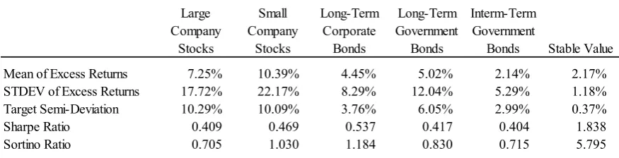
Mean of Excess Returns 7.25% 10.39% 4.45% 5.02% 2.14% 2.17%
STDEV of Excess Returns 17.72% 22.17% 8.29% 12.04% 5.29% 1.18%
Target Semi-Deviation 10.29% 10.09% 3.76% 6.05% 2.99% 0.37%
Sharpe Ratio 0.409 0.469 0.537 0.417 0.404 1.838
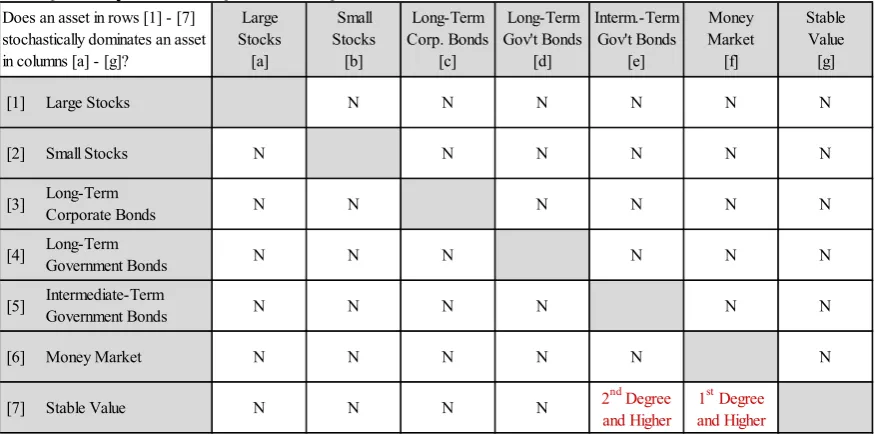
Table 4 presents the SD results among the seven asset classes in our study, based solely on historical returns.25 Only the SV historical returns distribution dominated two asset classes in
the stochastic dominance sense up to the fourth degree; none of the other asset classes domi-nates any other class of funds, including SV funds.
Table 4. Stochastic Dominance among Alternative Asset Classes. Net Quarterly Returns Q4-1988 – Q4-2015
Note: An entry of "N" indicates that the asset class in the corresponding row did not stochastically dominate the asset class in corresponding column in any of the first four degrees.
Turning to SV funds, they stochastically dominated money market investments by the first-degree and, as a corollary, by any higher first-degree as well. This is a direct consequence of the fact that when sorted returns for SV and money market funds are compared in a pairwise fashion over the past 27 years, the SV return was always greater than the corresponding money market return. In other words, the empirical cumulative distribution function (CDF) of the money market returns was strictly above and to the left of the empirical CDF of the SV returns, meaning that for any given return the probability of obtaining a lower return with a money market fund is greater than with an SV fund. Consequently, based on historical re-turns alone, any investor who preferred more wealth to less wealth should have avoided in-vesting in money market funds when SV funds were available, irrespective of risk prefer-ences. Of course, historical returns alone cannot establish dominance going forward, and expectations of future returns may well depend on factors not included by historical condi-tions.
Although SV funds failed to stochastically dominate intermediate-term government bonds by the first degree, they dominated by the second and higher degrees. This result is a direct con-sequence of the fact that while the empirical CDFs of these two asset classes cross (thus pre-venting first-degree stochastic dominance), positive intermediate-term bond returns during
25 Stochastic dominance analysis is not restricted to basing return and risk expectations solely on historical
returns, but that is the approach we take in this study. Large Stocks [a] Small Stocks [b] Long-Term Corp. Bonds [c] Long-Term Gov't Bonds [d] Interm.-Term Gov't Bonds [e] Money Market [f] Stable Value [g]
[1] Large Stocks N N N N N N
[2] Small Stocks N N N N N N
[3] Long-TermCorporate Bonds N N N N N N
[4] Long-Term
Government Bonds N N N N N N
[5] Intermediate-Term
Government Bonds N N N N N N
[6] Money Market N N N N N N
[7] Stable Value N N N N 2
nd
Degree and Higher
1st Degree and Higher
the period of our study were never large enough, relative to corresponding SV returns, to make at least some risk-averse investors prefer the riskier intermediate-term bond invest-ment. Technically, the integral of the difference between the intermediate-term bond return distribution and the SV return distribution is positive for any return.
The results in this sub-section are remarkable. Not surprisingly, there is no stochastic domi-nance of any one traditional class over another; indeed domidomi-nance is rarely encountered in empirical studies of asset classes. Accordingly, it was surprising to find that SV investments dominated two of the major traditional investment classes.
6.3 Intertemporal optimization analysis
In this section we look at the potential gains of including stable value funds in an investor’s portfolio when risk-aversion is explicitly taken into consideration and the investor maximizes expected utility of wealth in a dynamic setting. At the cost of making additional assumptions about an investor’s attitudes toward risk, this analysis provides additional insights into the role that stable value funds could play in portfolio design.
Our theoretical framework follows the intertemporal investment model of Grauer and Hakansson (1982, 1985, 1986, 1987, 1993, and 1995), considering an investor who, at the beginning of each period, allocates wealth among various investment alternatives so as to maximize expected utility of wealth. The investment alternatives we consider are the same as in our previous analysis, with investment horizon assumed to be a quarter. Therefore, the return data we use are net quarterly returns for the period Q1-1989 through Q4-2015.
In Grauer and Hakansson’s model (esp. 1982), new information about the distribution of as-sets is incorporated prior to each quarterly optimization and the utility-maximizing portfolio for the quarter is derived. More specifically, at the beginning of the optimization quarter t, the investor determines portfolio weights, , that maximize expected utility of wealth,
(1 + ) = (1 + ∑ ) (6)
subject to ≥ 0 for all i and ∑ = 1. E[·] is the expectations operator, wit is the
frac-tion of wealth allocated to investment i in period t, rit is the return on investment i over
quar-ter t, and a ≤ 1 is a risk paramequar-ter.26 The function U(·) is the constant relative risk aversion
(CRRA) utility function with coefficient of relative risk aversion given by = 1 − ≥ 0.
In Grauer and Hakansson (1982), the empirical distribution of returns is used to approximate the unknown joint distribution of returns. This approach is referred to as the “simple
26 For stable value and money market funds, the quarterly return is assumed to be known (declared crediting rate
bility assessment approach.” The authors use quarterly data over the 40 quarters (or ten years using annual data) prior to the optimization quarter (year) in order to compare the perfor-mance of the portfolio consisting of the series of optimal quarterly (or annual) portfolios over the 1936-1978 period (with data for the 1926-1978 period) with the performance over the same period of the individual asset classes they consider.
We examine data for 80 quarters prior to each optimization quarter.27 Given the historical
sample we employ, this means that our first optimization quarter is Q1-1993 and the last one is Q4-2015. Over these 92 quarters, a representative investor determines the optimal portfo-lio for each quarter, each time using the empirical distribution of returns from the immedi-ately preceding 80 quarters to maximize expected utility as described above. At the end of the 92 quarter period, the (geometric) average portfolio return and the standard deviation of returns are calculated for two portfolios, one that excludes stable value funds and another that includes them.
One empirical problem for this analysis is that bond yields have been decreasing steadily over the period examined and empirical past return averages for mostly any given quarter will therefore tend to overestimate the population expected future returns. For this reason, we modify Grauer and Hakansson’s simple probability assessment approach by estimating bond returns at the start of each optimization quarter with their respective yields (on a quar-terly basis). We do this for long-term corporate and government bonds and for intermediate-term government bonds. More specifically, for each of these bond series in each optimiza-tion quarter, the quarterly deviaoptimiza-tions from their respective means (over the previous 80 quar-ters) are added to the corresponding current bond yields (expressed as a quarterly return). In this way we preserve the joint co-movements of all assets classes subject to uncertain returns over each optimization quarter.28
We note that at the start of each optimization quarter, the expected return on the money-mar-ket and stable value funds is non-random. As indicated in Section 5 above, we use the yield on 3-month Treasury bills to approximate the expected returns on the money market fund and the promised crediting rate as the return on the stable value fund.
In a second piece of analysis, we focus on the last four quarters of 2015 and construct sce-narios for the expected return on large and small stock returns based on a range of assumed respective large and small equity premiums over money market yields.29 This allows us to
27 This was done to ensure that we captured multiple full business cycles in our estimations, as recently cycles
have lengthened markedly. (See, for example, http://www.nber.org/cycles.html) Because correlations across asset classes are sometimes quite different during the expansion portion of a cycle than during the contraction phase, robust estimations are best made across both phases of several full cycles.
28 An alternative that would take into account the term structure of interest is to employ a strict pure
expectations theory by setting the expected returns on all bond portfolios equal to their current quarterly certainty equivalent (i.e., the current quarterly Treasury bill rate) plus either a theory-based or a historical short-term risk spread. However, we felt there was no compelling justification to wed ourselves to one of several theories of the term structure of interest while introducing additional model error, and that the current bond yield adequately incorporated market expectations for purposes of this study.
simulate the performance of SV funds under various stock return scenarios during a period where crediting rates have been lowest due to the secular decline in interest rates.
Optimal Portfolio Returns Q1-1993 – Q4-2015
In this section the question of interest is what would be the (geometric) average quarterly return and volatility for a portfolio that is optimally rebalanced every quarter between 1993 and 2015, according to the rules set out above. We provide answers to this question for se-lected values of the risk aversion coefficient a in expression (6) above and for portfolios ex-cluding and inex-cluding stable value. Table 5 shows mean quarterly returns and standard devi-ations for each of these cases and Figure 4 illustrates the same results in the mean-standard deviation plane. The risk aversion values of a range from +1 to –75, the same range em-ployed by Grauer and Hakansson in their seminal papers.
The top panel in Table 5 reports the geometric mean returns and standard deviations of the various asset classes involved. These can be interpreted as portfolios that hold only one se-curity throughout the period 1993-2015 and so can be compared to the optimizing portfolios in the lower panel of Table 5, which shows the optimizing results across the whole spectrum of risk aversion levels.
Table 5. Geometric Quarterly Means and Standard Deviations for Optimal Portfolios, Q1-1993 through Q4-2015.
Mean STDEV
LS 1.91% 8.02%
SS 2.70% 11.04%
LTCB 1.59% 4.85%
LTGB 1.65% 5.59%
ITGB 1.04% 2.49%
MM 0.55% 0.52%
SV 1.13% 0.39%
Exclude SV Include SV
Value of a Mean STDEV Mean STDEV
1.00 2.70% 11.04% 2.70% 11.04%
0.75 2.63% 10.94% 2.63% 10.94%
0.50 2.52% 10.88% 2.52% 10.87%
0.25 2.29% 10.53% 2.29% 10.52%
0 2.14% 10.31% 2.14% 10.31%
−1 1.98% 8.99% 1.97% 8.99%
−2 1.97% 7.58% 1.91% 7.45%
−3 1.96% 6.53% 1.92% 6.07%
−5 1.85% 5.00% 1.81% 4.10%
−7 1.76% 4.22% 1.68% 3.10%
−10 1.58% 3.45% 1.54% 2.26%
−15 1.30% 2.40% 1.42% 1.57%
−20 1.13% 1.83% 1.35% 1.21%
−25 1.02% 1.49% 1.31% 0.99%
−30 0.95% 1.27% 1.29% 0.85%
−40 0.85% 0.99% 1.25% 0.68%
−50 0.79% 0.84% 1.23% 0.58%
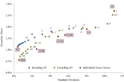
In figure 4 we plot the optimal risk-return pairs in Table 5. More specifically, we plot mal portfolios for selected risk-aversion parameters when SV returns are included and opti-mal portfolios when SV returns are excluded. We also plot with the geometric mean returns and standard deviations, over the same period, Q1-1993 through Q4-2015, for the asset clas-ses we consider.
Figure 4 – Optimal Portfolios for Selected Risk Aversion Parameters, Excluding and Includ-ing Stable Value Assets
The case where the risk parameter a equals 1 is that of linear utility and risk is of no concern to the risk-averse investor. Since in our sample, average returns for all quarters in 1993-2015 (based in the previous 80 quarters of data) are highest for small stocks (SS), the sequence of optimal portfolios implies holding small stocks throughout the period, excluding any other asset class, and obtaining a geometric average quarterly return of 2.70% and a quarterly standard deviation of 11.04%.
The inclusion of stable value assets in the mix of asset classes begins to make a difference with risk parameter of a = −2 (corresponding to a coefficient of relative risk aversion of ρ = 1 – a = 3). In particular, we observe that the inclusion of stable value reduces the portfolio’s average standard deviation for risk parameter less than or equal to −2 and increases the geo-metric mean return for values of the risk parameter less than or equal to −15. For this case, the quarterly average portfolio return is 1.42% and the average standard deviation is 1.57% when stable value is included, compared to 1.30% and 2.40% when excluded.
Figure 5-A – Optimal Allocations by Quarter for Risk Parameter a = 0 (Excluding SV)
Figure 5-B – Optimal Allocations by Quarter for Risk Parameter a = 0 (Including SV)
Besides these two cases where the degree of risk aversion is nonexistent or low, relevant questions are, therefore, at what level of risk aversion do lower-yielding assets begin to play a significant role in optimal portfolios and, specifically for our inquiry, at what level of risk aversion do stable value investments begin to play a significant role in optimal portfolios and what other assets classes do they replace when included. Figures 6 through 8 below provide an answer to these questions.
around 1995 and 1996 (Figure 6-A). When stable value funds are included (Figure 6-B), they entirely replace intermediate-term government bonds and money market funds. Inter-estingly, stable value funds also partially replace small stocks in the 1993-1997 sub-period and some long-term corporate bonds around 1993-1994 and 2003-2004.
Figure 6-A – Optimal Allocations by Quarter for Risk Parameter a = −2 (Excluding SV)
Figure 6-B – Optimal Allocations by Quarter for Risk Parameter a = −2 (Including SV)
Figure 7-A – Optimal Allocations by Quarter for Risk Parameter a = −5 (Excluding SV)
Figure 8-A – Optimal Allocations by Quarter for Risk Parameter a = −10 (Excluding SV)
Figure 8-B – Optimal Allocations by Quarter for Risk Parameter a = −10 (Including SV)
Sensitivity to Expected Stock Returns
In the previous analysis we have used historical returns for large and small US stocks in modelling the joint distribution of quarterly returns. There is, however, an ongoing discus-sion about what the equity premium may be in the future (Fernández et al, 2015, 2017), sug-gesting that past historical equity premiums may not be an accurate estimate of future equity premiums. This observation echoed that presaged by Siegel (2005) some ten years earlier. In this section we conduct a scenario analysis in which we use three levels of the equity pre-mium, 3%, 5%, and 7% per year, over the money market yield for each optimization quarter. Therefore, the expected return for a given optimization quarter in a given scenario is con-structed as the promised 3-month yield plus the scenario’s large stock equity premium (3%, 5%, or 7%). For small stocks, we add the historical average return spread between small and large stocks over the 80 quarters of data used for each optimizing quarter to the correspond-ing expected large stock return just described.
As in the previous section, we preserve the co-movement of the asset classes considered by adding the quarterly deviations of historical returns from their respective sample means to their current modeled expected returns for large and small stocks, long-term government and corporate bonds, and intermediate-term government bonds.
Figures 9-11 show the asset weights of optimal portfolios for the three large stock equity premium scenarios considered, at selected risk parameters and varying assumed equity premia for the four quarters of 2015.30
30 For the sake of brevity only results for 2015 are shown here. Complete results for all years in the period 1993
Figure 9-A – 2015 Optimal Portfolios (LS Equity Premium = 3%) – Excluding SV
Q1 Q2 Q3 Q4 Q1 Q2 Q3 Q4 Q1 Q2 Q3 Q4 Q1 Q2 Q3 Q4 Q1 Q2 Q3 Q4
Figure 9-B – 2015 Optimal Portfolios (LS Equity Premium = 3%) – Including SV
Figure 10-A – 2015 Optimal Portfolios (LS Equity Premium = 5%) – Excluding SV
Q1 Q2 Q3 Q4 Q1 Q2 Q3 Q4 Q1 Q2 Q3 Q4 Q1 Q2 Q3 Q4 Q1 Q2 Q3 Q4
Figure 10-B – 2015 Optimal Portfolios (LS Equity Premium = 5%) – Including SV
Figure 11-A – 2015 Optimal Portfolios (LS Equity Premium = 7%) – Excluding SV
Q1 Q2 Q3 Q4 Q1 Q2 Q3 Q4 Q1 Q2 Q3 Q4 Q1 Q2 Q3 Q4 Q1 Q2 Q3 Q4
Figure 11-B – 2015 Optimal Portfolios (LS Equity Premium = 7%) – Including SV
Q1 Q2 Q3 Q4 Q1 Q2 Q3 Q4 Q1 Q2 Q3 Q4 Q1 Q2 Q3 Q4 Q1 Q2 Q3 Q4
7. Robustness Analysis
While important, the implications of our three-fold analysis should not be regarded as dis-positive. It should be recalled that over the 27-year period of the first phase of our analysis, which began with the inception of modern SV funds in 1989, interest rates exhibited a gen-eral decline to half their initial level, albeit with occasional and protracted periods of rising interest rates interspersed. Such a period of decline would tend to favor longer duration fixed income investments, including stable value, over money market funds. We sought to remedy this by including the precursors of SV funds – traditional GICs – to see how they fared dur-ing the period of rapidly risdur-ing interest rates that characterized the late 1970s and early 1980s. 31
Table 6 reports summary statistics for the extended period Q2-1973 through Q4-2015. Table 6. Summary Statistics – Net Quarterly Returns, Q2-1973 – Q4-2015
Note 1: The Jarque-Bera (JB) test is a test of the null hypothesis of normality. When the null hypothesis is true, the JB statistic has an approximate chi-square distribution with two degrees of freedom. 5%, 1% and 0.1% critical values are, re-spectively, 5.99, 9.21, and 13.82.
Note 2: The JB test assumes independent returns. This is a reasonable assumption for all but money market and stable value returns and we do not apply the test to these data.
Comparing Tables 1 and 6, we observe that average returns for a particular asset class vary considerably, especially for small stocks, money market, intermediate-term governments, and SV returns. Small stocks have an average net quarterly return of 3.98% for the extended period, compared with 3.27% for the period Q4-1988 through 2015. This difference is es-sentially due to the better performance of small stocks over the period 1973–1988 and the smaller impact of the negative returns in 2008 on an average calculated over 171 quarters instead of 109. The 46 basis points jump in money market quarterly average return for the extended period is due to the higher yields on debt instruments observed during the late
31 Many SV funds use the Lehman Intermediate Government/Credit Bond yield series as a benchmark. We use
the wrapped index based on this series (provided to us by the SVIA, for the period of February 1973 through February 2008) as our proxy for SV returns prior to the beginning of our SV average return series in Q4-1988. More specifically, we regress the series of quarterly SV returns on the Lehman intermediate government/credit wrapped series quarterly returns over the period Q4-1988 through Q4-2007 (the period during which the two series’ quarterly returns overlap) and extrapolate the SV return series for the period Q2-1973 through Q3-1988.
Large Company Stocks Small Company Stocks Long-Term Corporate Bonds Long-Term Government Bonds Interm-Term Government Bonds Money
Market Stable Value
Mean 2.43% 3.98% 1.85% 1.88% 1.46% 1.21% 1.54%
Median 2.71% 4.28% 1.36% 0.97% 1.03% 1.23% 1.53%
Maximum 22.37% 44.26% 23.71% 23.85% 16.06% 3.93% 2.64%
Minimum -25.74% -28.47% -13.73% -15.02% -6.86% -0.05% 0.44%
Std. Dev. 8.33% 12.11% 5.47% 6.03% 3.12% 0.92% 0.58%
Skewness -0.548 0.025 0.707 0.779 1.032 N/A N/A
Kurtosis 0.880 0.570 2.939 1.711 3.125 N/A N/A
Jarque-Bera 8.973 1.487 48.293 24.313 63.686 N/A N/A
enties and early eighties. This is also the reason that the SV quarterly average return in-creased by 26 basis points to 1.54% for the extended period compared to the average of 1.28% over the period Q4-1988-2015. Intermediate-term governments had an average in-crease of 24 basis points.
Mean-Variance Analysis
The differences we observe in mean returns across the two sample periods considered are reflected in the efficient frontier corresponding to the Q2-1973 through Q4-2015 data, shown in Figure 12, contrasted with Figure 3 earlier.
Figure 12. Efficient Frontiers for Alternative Asset Classes (Q2-1973 – Q4-2015)
We observe a much flatter efficient frontier for the extended sample period. This is primarily the result of the higher small stocks average return compared to its corresponding value for the Q4-1988 – Q4-2015 sample period.32
32 An important factor in the degree of curvature of the efficient frontier is the correlation among asset classes.
Table 7-A reports these efficient portfolios for selected points along the efficient frontier. We observe that the composition of the efficient portfolios reported earlier in Table 2-A changes in some respects when the extended sample is considered here, but it also remains the same in other respects. Table 7-A (covering the extended period) shows that large stocks, long-term corporate bonds, intermediate-term bonds and money market assets are completely excluded from the efficient frontier whereas in the Q4-1988 – Q4-2015 sample reported in Table 2-A, large stocks had at least a slight participation and in one case (at the lowest risk level) long-term corporates even entered the efficient frontier marginally. We also observe that the weights of SV funds are markedly larger than for the portfolios shown in Table 2-A. Table 7-A. Optimal Weights for Mean-Variance Efficient Portfolios Including SV
(Q2-1973 – Q4-2015)
Another important difference with Table 2-A is that the weight of long-term government bonds is now much decreased (from an average holding of30% to 20%) across all efficient portfolios and the weight of small stocks is correspondingly increased.
Table 7-B repeats the optimal portfolio analysis but where SV is not included as an available asset class. We observe that money market instruments enter the optimal portfolios at vari-ous levels of portfolio risk, along with small stocks and long-term government bonds. How-ever, unlike the results of the shorter period shown in Table 2-B, intermediate-term bonds no longer enter the optimal portfolios at any levels of portfolio risk even though there is no SV to dominate them. We also observe that large stocks and long-term corporates enter mean-variance-efficient portfolios only once, at the lowest expected return and standard deviation combination, when calibrations are based on the past 43 years of historical returns and
cor-Expected Return
Standard
Deviation Large Stocks Small Stocks
Long-Term Corp. Bonds Long-Term Gov't Bonds Interm.-Term Gov't Bonds Money
Market Stable Value
1.54% 0.58% 0.00% 0.07% 0.00% 0.00% 0.00% 0.00% 99.93%
1.66% 0.81% 0.00% 4.63% 0.00% 3.13% 0.00% 0.00% 92.23%
1.79% 1.28% 0.00% 9.17% 0.00% 6.45% 0.00% 0.00% 84.38%
1.91% 1.80% 0.00% 13.71% 0.00% 9.76% 0.00% 0.00% 76.53%
2.03% 2.34% 0.00% 18.25% 0.00% 13.07% 0.00% 0.00% 68.68%
2.15% 2.89% 0.00% 22.79% 0.00% 16.38% 0.00% 0.00% 60.83%
2.27% 3.45% 0.00% 27.33% 0.00% 19.69% 0.00% 0.00% 52.98%
2.39% 4.01% 0.00% 31.86% 0.00% 23.00% 0.00% 0.00% 45.13%
2.52% 4.57% 0.00% 36.40% 0.00% 26.32% 0.00% 0.00% 37.28%
2.64% 5.14% 0.00% 40.94% 0.00% 29.63% 0.00% 0.00% 29.43%
2.76% 5.70% 0.00% 45.48% 0.00% 32.94% 0.00% 0.00% 21.58%
2.88% 6.26% 0.00% 50.02% 0.00% 36.25% 0.00% 0.00% 13.73%
3.00% 6.83% 0.00% 54.56% 0.00% 39.56% 0.00% 0.00% 5.88%
3.12% 7.39% 0.00% 59.41% 0.00% 40.59% 0.00% 0.00% 0.00%
3.25% 7.99% 0.00% 65.21% 0.00% 34.79% 0.00% 0.00% 0.00%
3.37% 8.62% 0.00% 71.01% 0.00% 28.99% 0.00% 0.00% 0.00%
3.49% 9.28% 0.00% 76.81% 0.00% 23.19% 0.00% 0.00% 0.00%
3.61% 9.97% 0.00% 82.61% 0.00% 17.39% 0.00% 0.00% 0.00%
3.73% 10.67% 0.00% 88.40% 0.00% 11.60% 0.00% 0.00% 0.00%
3.85% 11.38% 0.00% 94.20% 0.00% 5.80% 0.00% 0.00% 0.00%
3.98% 12.11% 0.00% 100.00% 0.00% 0.00% 0.00% 0.00% 0.00%
Note: Weights may not add up to 100% across a given row due to rounding.
relations. Finally, in comparing the first two columns of Table 7-A with the corresponding columns in Table 7-B, we see by using simple interpolation that for most given expected returns in a portfolio precluded from SV assets, the risk is higher than for the case when SV is included.
Table 7-B. Optimal Weights for Mean-Variance Efficient Portfolios Excluding SV (Q2-1973 – Q4-2015)
Sharpe and Sortino Ratios
Comparable Sharpe and Sortino ratios are calculated for the extended sample and reported in Tables 8-A and 8-B below.
We note that unlike the shorter period (Q4-1989 through Q4-2015), during which the money market rate exceeded the SV rate in four out of the 109 quarters in the period (about 3.7% of the time), the extended period of 171 quarters contained 30 quarters (about 17.5% of the time) during which money market yields exceeded the corresponding SV rates. It is there-fore interesting to observe that extending the sample to include a period of significantly
Expected Return
Standard
Deviation Large Stocks Small Stocks
Long-Term Corp. Bonds
Long-Term Gov't Bonds
Interm.-Term Gov't Bonds
Money Market 1.23% 0.91% 1.09% 0.02% 1.30% 0.00% 0.00% 97.59% 1.37% 1.04% 0.00% 4.52% 0.00% 5.09% 0.00% 90.38% 1.51% 1.38% 0.00% 8.43% 0.00% 9.42% 0.00% 82.15% 1.64% 1.80% 0.00% 12.34% 0.00% 13.74% 0.00% 73.92% 1.78% 2.27% 0.00% 16.24% 0.00% 18.06% 0.00% 65.69% 1.92% 2.76% 0.00% 20.19% 0.00% 22.43% 0.00% 57.38% 2.06% 3.26% 0.00% 24.10% 0.00% 26.75% 0.00% 49.15% 2.19% 3.76% 0.00% 28.01% 0.00% 31.07% 0.00% 40.92% 2.33% 4.27% 0.00% 31.92% 0.00% 35.40% 0.00% 32.69% 2.47% 4.78% 0.00% 35.82% 0.00% 39.72% 0.00% 24.46% 2.60% 5.30% 0.00% 39.77% 0.00% 44.09% 0.00% 16.14% 2.74% 5.82% 0.00% 43.68% 0.00% 48.41% 0.00% 7.91% 2.88% 6.34% 0.00% 47.69% 0.00% 52.31% 0.00% 0.00% 3.02% 6.90% 0.00% 54.21% 0.00% 45.79% 0.00% 0.00% 3.15% 7.53% 0.00% 60.73% 0.00% 39.27% 0.00% 0.00% 3.29% 8.22% 0.00% 67.32% 0.00% 32.68% 0.00% 0.00% 3.43% 8.94% 0.00% 73.84% 0.00% 26.16% 0.00% 0.00% 3.56% 9.70% 0.00% 80.37% 0.00% 19.63% 0.00% 0.00% 3.70% 10.48% 0.00% 86.89% 0.00% 13.11% 0.00% 0.00% 3.84% 11.28% 0.00% 93.41% 0.00% 6.59% 0.00% 0.00% 3.98% 12.11% 0.00% 100.00% 0.00% 0.00% 0.00% 0.00%
Note: Weights may not add up to 100% across a given row due to rounding.