Route referencing and ordering for synchronization free delay tomography in wireless networks

R E S E A R C H

Open Access

Route referencing and ordering for

synchronization-free delay tomography in

wireless networks

Kensuke Nakanishi

, Teruhito Naka

, Shinsuke Hara

, Takahiro Matsuda

, Kenichi Takizawa

, Fumie Ono

and Ryu Miura

Abstract

Delay tomography is an inference technique for link delays in a network, where end-to-end route measurement is a promising method to reduce measurement overhead. Furthermore, by incorporating compressed sensing, delay tomography can efficiently detect sparse anomaly. In delay tomography, however, there is an inevitable issue that is clock synchronization for the route measurements. In this paper, based on route referencing, we study synchronization-free delay tomography with compressed sensing. From theoretical analysis, optimal route referencing and ordering methods for synchronization-free delay tomography are derived as “subtractive and differential schemes,” which cancel or minimize the error factors caused by clock asynchronism, clock skew, and normal link delays with single or multiple references, respectively. Simulation experiments confirm that the proposed methods can identify abnormal links more accurately with robustness against the error factors than a conventional scheme, where the newly proposed differential scheme always shows the best performance thanks to its better error

factors cancelation.

Keywords: Anomaly detection, Compressed sensing, Network tomography, Synchronization-free delay tomography

1 Introduction

Anomaly detection/identification [1] is essential for wire-less sensor networks since it can guarantee not only long-term workability but also quick recovery once an anomaly occurs. In order to detect and identify anomaly, it is nec-essary to monitor the network either passively, actively, or both. In a passive approach, the traffic flows on the net-work are passively monitored and the netnet-work informa-tion is collected. There are a number of routing algorithms proposed for wireless sensor networks [2], and among them, distributed algorithms are commonly used for their low transmission redundancy. In distributed routing algo-rithms, each sensor node locally exchanges hello packets for link state probing only between the neighboring sensor nodes, and then, data packets of each sensor node are sent according to the established routes in the network. This

*Correspondence:[email protected]

1_{Wireless System Laboratory, Corporate Research & Development Center,}

Toshiba Corp., 212-8582 Kanagawa, Japan

Full list of author information is available at the end of the article

implies the drawback of the passive network monitoring, that is, it is limited to the periods of time when there is traffic on the network between the nodes of interest. On the other hand, an active approach that injects traffic into the network can quickly and accurately detect anomaly, but may adversely affect the normal data traffic. The pri-mary purpose of wireless sensor networks is to reliably collect data from sensor nodes, so it should be accom-plished by fewer probing packets and less interference for normal data traffic without change or addition of sensor network functions. In this paper, we address the chal-lenge of the active anomaly detection in an asynchronous network, based on “network tomography [3–5].”

Network tomography has been used to encompass a class of approaches to estimate internal link states from end-to-end route measurements in networks. Especially when packet route delays are measured, network tomog-raphy is referred to as “delay tomogtomog-raphy,” and recently, it has been applied to the problem of anomaly iden-tification in networks since it alleviates cooperation of internal nodes. In the problem, tomography schemes

are often formulated as underdetermined linear systems [6–8], and compressed sensing [9,10] is utilized to solve it, which is a promising technique for reconstructing a finite-dimensional sparse vector based on its linear mea-surements with dimension smaller than the size of the unknown sparse vector. The probability that multiple anomaly simultaneously occur is considered to be rela-tively low, so compressed sensing has successfully brought high efficiency into delay tomography for the aforemen-tioned challenge of the active anomaly detection, by reducing the number of measurement routes as compared to the number of links in a given network, that is, by reducing the number of probing packets. Similar to the previous study [6–8], provided that the sparsity of the desired solution can be exploited, the primary objective of this paper is to identify few links giving extraordinarily large delays as anomaly, which is referred to as “abnormal links.”

In a wireless sensor network, unattended sensor nodes are usually likely to connect to neighboring nodes in bet-ter link states, so it is difficult for its network manager to know whether there is something wrong in a network and where it is even if they notice it. When an anomaly happens due to a node failure, the active delay tomogra-phy can identify it, so the manager can fix or replace the failed node. This would be necessary for continuing the task of the wireless sensor network. In addition, when an anomaly happens due to a link disconnection by a physical obstruction, the manager can find or remove the physical obstruction for the identified link. This would be applica-ble for an intruder or wild animal detection in a wireless sensor network for environmental monitoring over an agricultural field. Although delay tomography brings these benefits into wireless sensor networks, few works have been dedicated for this interesting research topic [11–15]. As an issue for consideration, delay tomography bur-dens source and destination nodes with clock synchro-nization between them. A packet route delay, which is required in the formulation, can be known from the transmission time at a source node and the reception time at a destination node, so precise clock synchro-nization between them seems essential and unavoidable, but it is difficult in reality. In wireless sensor networks, the electronic components of nodes are sometimes too untrustable to meet the requirement of clock synchro-nization in terms of precision and complexity [16, 17]. Global positioning system (GPS) may provide precise clock synchronization among wireless nodes [18], but all nodes cannot be equipped with GPS receivers. Network time protocol (NTP) [19] is applicable and several meth-ods using the medium access control layer (MAC) time stamp [20–22] have been proposed for clock synchro-nization, but they require all nodes to exchange packets specialized for clock synchronization. It must be more

energy-efficient to accomplish active delay tomography without the use of such specialized packets.

In [13], we tackled the clock synchronization problem and proposed a synchronization-free delay tomography based on compressed sensing. The proposed scheme can-cels the time offset between the source and destination nodes by selecting a single reference route, inspired by the workability of a time-difference-of-arrival (TDOA)-based localization where the clocks of target node and refer-ence nodes are not synchronized [18]. The trade-off for the asynchronism is a loss of equation in the delay tomog-raphy formulation, but compressed sensing is a method to obtain a solution from an underdetermined linear sys-tem, so it successfully compensates the trade-off. In [13], based on the compressed sensing theory, the potential performance is discussed for identifying abnormal links when measurement routes are given, and it is proven that the potential performance can be preserved, as long as reconstructing an underdetermined exactly sparse vector with a single non-zero entry. Here, we refer to the con-ventional synchronization-free delay tomography scheme with a single route reference as “a subtractive scheme.”

In addition to the success of the cancelation of the time offset in asynchronous wireless sensor networks, it needs to be carefully designed taking two more factors into con-sideration in order to more accurately identify abnormal links, which are inherent to wireless sensor networks. One is “link delay,” which always arises from some fac-tors: buffering, medium access protocol, packet collision, and packet loss due to propagation characteristics such as fading, blocking, and near/far effect. The link delay in wireless networks is relatively large as compared to that in wired networks and is accumulated in the measured route delay as a large positive bias, so it gives an unig-norable impact on the tomography performance, if the route delays are simply used in it. The other is clock error derived from clock frequency deviation, which is referred to as “clock skew.” Since the frequency of crystal oscilla-tors inevitably deviates [23], the clock error between the source and destination nodes increases over time even if the clock of one node is temporarily synchronized to that of the other node at a time. For example, when the mea-surement interval gets longer to avoid interference from active probing packets to normal data traffic, the clock skew appears as a larger time-variant bias in the mea-sured route delay. In [24], we simply analyzed the effect of the two error factors but did not deeply discuss the performance of the subtractive scheme.

subtractive scheme. Next, extending the idea to the case of multiple routes reference, we newly propose a better synchronization-free delay tomography scheme, which is referred to as “a differential scheme,” with its optimal route referencing and ordering method as well. We show by sim-ulation experiments that well-designed synchronization-free delay tomography schemes can be insensitive to the error factors and accurately identify abnormal links in an asynchronous wireless network. To the best of the authors’ knowledge, there have been no works on the theoreti-cal analysis of such error factors and the design of route referencing and ordering suited for delay tomography in wireless sensor networks, although there are a number of works dealing with network tomography.

The remainder of this paper is organized as follows. Section 2 presents some preliminaries on compressed sensing for discussing the mathematical property of the proposed schemes. Section3explains the system model. After Section4introduces the conventional delay tomog-raphy. Sections5and6propose the synchronization-free delay tomography methods with a single route refer-ence and multiple routes referrefer-ence, respectively. Section7 prepares to evaluate the proposed methods, and then, Section8demonstrates their performance by simulation experiments. Finally, Section9concludes the paper.

2 Preliminaries on compressed sensing 2.1 Definition

The p norm (p ≥ 1) of a vector ω =[ω1,ω2,· · ·,ωj,

· · ·,ωJ]∈RJ×1is defined as

ωp=

⎛ ⎝J

j=1

|ωj|p

⎞ ⎠

1 p

(1)

wheredenotes the transpose operator. Forp=0, using its support, we defineω0as

ω0 = |supp(ω)| (2)

supp(ω) = {j|ωj=0}. (3)

K-sparse vectors are defined as those which have at mostKnon-zero elements, and a set ofK-sparse vectors K ∈RJ×1is given by

K =

ω∈RJ×1_{| ω} 0≤K

. (4)

We consider that, through a matrixA∈RI×J (I <J), a linear measurement vectory =[y1,y2,· · ·,yi,· · ·,yI]∈

RI×1_{for a vectorx =[x}

1,x2,· · ·,xj,· · ·,xJ]∈ RJ×1 is

obtained as

y=Ax. (5)

Whether or not one can recover a sparse vectorxfrom y by means of compressed sensing can be evaluated by Spark (A), which is defined as

Spark(A)= min

ω∈Ker(A)\{0}ω0 (6)

where Ker(A)denotes the kernel ofA, that is,

Ker(A)=ω∈RJ×1|Aω=0. (7) The following theorem guarantees the unique recover-ability of sparse vector [10]:

Theorem 1For anyy, there exists at most onex∈ K

such thaty=Ax, if and only if Spark(A) >2K .

Theorem 1 yields the requirement I ≥ 2K, since Spark(A) ∈ [2, I+1]. We refer to such a matrixAwith Spark(A) >2KasK-identifiable.

2.2 0,1, and1/2optimization problems

WhenAisK-identifiable andyis not contaminated with noise in (5), x ∈ K is reconstructed by solving the

following0optimization problem:

ˆ

x=argmin

x∈RJ×1

x0 subject to y=Ax. (8)

Because of the discrete and discontinuous nature of the

0, it is very difficult to solve (8), so instead, the following

1relaxation of (8) is proposed:

ˆ

x=argmin

x∈RJ×1

x1 subject to y=Ax. (9)

The problem given by (9) can be easily solved by lin-ear programming algorithms, and its solution is proven to be equivalent to the one for the original0optimization

problem [25].

On the other hand, whenyis contaminated with some form of noise, Theorem1may not guarantee the recover-ability. In this case, instead, we estimatexˆby solving the following1/2optimization problem [26,27]:

ˆ

x=argmin

x∈RJ×1 1

2y−Ax

2

2+ξx1

(10)

whereξis an adjustable parameter.

Several methods have been so far proposed to solve the1/2optimization problem [10], and we use the fast

iterative shrinkage-thresholding (FISTA) algorithm [28] to obtainxˆ. In our simulation experiments, after select-ing the element with the maximal magnitude from the elements ofxˆ asxmax, we finally identify the indexes of

ˆj= {j| |xj| ≥θxmax} (11)

whereθis a constant parameter.

3 System model

3.1 Network and tomography session model

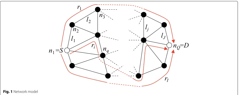
Figure1shows the network model with a defined bound-ary. Let G = (N,L) denote an undirected network, whereN andL ⊂ N ×N are sets of nodes and links, respectively1_{. The nodes and links are numbered such as} N = {n1,n2,· · ·,nq, · · ·,nQ} and L =

{l1,l2,· · ·,lj,· · ·,lJ}, where Q = |N| and J = |L|

denote the numbers of nodes and links, respectively. It is assumed that the topology is fixed while a tomography session defined below is conducted.

We consider delay tomography in a simple scenario [7,13] for an easy-to-understand explanation, where a sin-gle source node S and a single destination node D are assigned out of the boundary nodes, and S has estab-lished several routes to Dbefore a tomography session. We define a set of the routes asR= {r1,r2,· · ·,ri,· · ·,rI},

where I denotes the number of routes, and define a set of links which constitutesri asLi. In a tomography

ses-sion,S sequentially sends probing packets toDthrough the routes in the packet transmission interval of T_probe. Here, in order for a probing packet to traverse over each pre-selected route,Suses a source routing algorithm such as the dynamic source routing (DSR) [29].

For each of the probing packets, the corresponding end-to-end delay is calculated from the transmission time atS

and reception time atD. Note that, since the active prov-ing traffic increases the load of the network, its longer transmission interval is preferable not to interfere with normal data traffic; on the other hand, since the assump-tion of the staassump-tionarity in the network may be invalid for

a long duration, the tomography session should be per-formed in a short time. One of the reasons for utilizing compressed sensing is that it is possible to reduce the number of probing packets while keeping the identifiabil-ity of abnormal links.

In addition to the above definitions and notations, we assume that there areKabnormal links giving extraordi-narily large delays in the network. The abnormal links are distinguished from the other links referred to as normal links, and they are separated into different setsLAandLN withLA = K andLN = J−K, respectively. Finally, we define sets of routes containing and not containing abnormal links asRAandRN, respectively, and define the numbers of abnormal links and normal links overriasκi

(κi≤K) andρi, respectively.

3.2 Clock model

Figure2shows a clock model. On the basis of the clock ofS, the clocks ofSandDare written respectively as

tS = t (12)

tD = αt+Toff =( sk+1)t+Toff (13)

whereT_off and _sk =(α−1)are the time offset att=0 and the skew parameter, respectively. As an example of clock skew, in the IEEE 802.11 standard for wireless local area networks (WLANs) and the IEEE 802.15.4 standard for wireless personal area networks (WPANs), the physi-cal layer (PHY)/medium access control (MAC) protocols are designed to accept the clock error up to ±40 ppm [30,31]. In this paper, assuming that the clock frequency uniformly deviates in [− dev,+ dev], skfollows the

tri-angular distribution tritri-angular [−2 dev, 0,+2 dev] with

the following average and variance:

Fig. 2Clock model

E[ sk] = 0 (14)

E 2_sk = 2

3

2

dev (15)

whereE[(·)] is the ensemble average of(·).

3.3 Link delay model

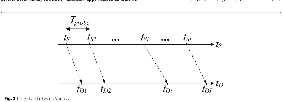
Figure3shows the time chart betweenSandD. Theith probing packet (i=1, 2,· · ·,I), which is transmitted from

S at time of tSion the basis of the clock of S, traverses

theith route and finally arrives atDat time oftDion the

basis of the clock ofD. It experiences the delay ofzi on

the basis of the clock of S, which is the sum of the link delays over the ith route. In [6], it is assumed that the normal link delay behaves stochastically according to an exponential distribution whereas the abnormal link delay behaves deterministically, irrespective of wired or wire-less networks. In this paper, we take the same approach as in [6], but we adopt a different model on the normal link delay suited for wireless sensor networks [32], that is Gaussian distribution. The reason is due to the cen-tral limit theorem, which asserts that the distribution of the sum of a large number of independent and identically distributed (i.i.d.) random variables approaches to that of

Gaussian random variable. This model will be appropriate if the link delays are thought to be the addition of numer-ous independent random processes. So whenljis a normal

link, that is,lj ∈LN, we assume that its delay is given as a

Gaussian random variableγj, and it is i.i.d. among links.γj

has the following statistical properties:

Eγj = ηN (16)

E

γ2

j

= η2

N+σN2 (17)

where ηN and σN2 are the average and variance of γj, respectively. On the other hand, for an abnormal

link lj ∈ LA, we assign a constant large delay of ηA

ηA ηN, η2A σN2

. Finally, as the statistical proper-ties of the link states, we assume that the link delays are stationary in a tomography session.

4 Conventional delay tomography scheme 4.1 Matrix/vector representation

The measured route delay overri(i = 1, 2,· · ·,I) can be written as

yi = tDi−tSi

= zi+Toff + sk(tSi+zi) (18)

zi =

lj∈Li

dj. (19)

Defining the link delay vectord∈RJ×1as

d=[d1,d2,· · ·,dj,· · ·,dJ], (20)

it can be decomposed into the following two vectors:

d = x+a (21)

x= [x1,x2,· · ·,xj,· · ·,xJ] (22)

a = [a1,a2,· · ·,aj,· · ·,aJ] (23)

where x ∈ RJ×1 and a ∈ RJ×1 are the link delay vec-tors containing only the abnormal link delays whereas the normal link delays, respectively, that is,

dj = xj+aj (24)

Furthermore, defining the measurement route delay vectory∈RI×1, the routing matrixB∈ {0, 1}I×J, theith

the measurement route delay vectoryis written as

y=Bx+Ba+v+w. (34)

Now, the purpose of the tomography is to estimate theK

non-zero elements ofx, so we distinguish betweenxand the other vectors which are the components oferror factor

vectordefined as

is the route delay vector contributed from normal links u∈RI×1. Consequently, we arrive at

y=Bx+e. (37)

4.2 Design for reducing the effect of the error factors Let us pay attention to the statistical properties of e. Regarding the each component ofe, from (16), (17), and (36), the statistical properties of theith element ofuare calculated as

from (32), the statistical properties of theith element ofv are written as

E[vi] = Toff (40)

Ev2_i = T_off2 (41)

and from (14), (15), and (33), the statistical properties of theith element ofware written as

E[wi]=0 (42)

Thus, taking into consideration

εww

where PA and PN are the probabilities that ri (i =

1, 2,· · ·,I) is included inRAandRN, respectively. From these, in order for a conventional scheme to perform the delay tomography accurately, in other words, to minimize the mean squared norm ofegiven by (46), there is no way except for selecting clock oscillators with high clock fre-quency stabilities dev≈0 and estimating the time offset

accurately to makeToff ≈0.

5 Subtractive scheme 5.1 Matrix/vector representation

The subtractive scheme is achieved by getting rid ofToff

completely, where themth row components ofy,B,u, and ware selected as references. Define a set of observation route indexes asIroute = {1, 2,· · ·,I}with |Iroute| = I.

Using Iroute, sets of selected reference route indexes Frefand not-selected (remaining) route indexesHremare

defined respectively as

route delay vector contributed from normal linksuref ∈

R(I−1)×1_{, the reference clock skew vectorw}

ref∈R(I−1)×1,

the remaining route delay vector yrem ∈ R(I−1)×1, the

remaining routing matrixBrem∈R(I−1)×J, the remaining

route delay vector contributed from normal linksurem ∈

R(I−1)×1_{, and the remaining clock skew vector w}

Therefore, we finally have the following new matrix/vector equation:

tractive routing matrix using themth route reference and v disappears completely in (68). Note that, in [13], the principle of the synchronization-free delay tomography corresponding to (65)–(67) was simply derived, but it seemed that mcan be neither 1 nor I. The expressions from (55) to (70) seem complicated but are more math-ematically strict and expandable for the case of multiple routes reference. When u(m) ≈ 0andw(m) ≈ 0, (65), (66), and (67) result in the equations which are indeed equivalent to those in [13].

5.2 Reference route selection preserving the identifiability

Assuminge(m) =0in (65), it becomes a simple equation of linear observation (see (5)). In [13], it is proven that, ifB is 1-identifiable, thenB(m) can be also 1-identifiable, and in this case, we can identify the abnormal link by solving the 1optimization problem (see (9)). Now, we add the

following two theorems to the synchronization-free delay tomography scheme.

Theorem 2If the subtractive routing matrix using the

m1th route reference is K-identifiable, then another

sub-tractive routing matrix using the m2th route reference is

also K-identifiable.

ProofSee the Appendix1.

Theorem 3If a subtractive routing matrix is K-identifiable and the number of abnormal links is more than K, then we can have the same possibility to identify them even when selecting any route as the reference.

ProofSee the Appendix2.

In reality, however, the assumption ofe(m) = 0cannot be held in (65), and in this case, we can identify the abnor-mal link by solving the1/2 optimization problem (see

(10)).e(m)varies according to the reference and order of the probing routes, so the solution is still affected by the design of the tomography session. In the following sub-sections, how to order the measurement routes and select a preferable reference is addressed to makeEe(m)e(m) closer to 0.

5.3 Reference route selection for reducing the error factors to (74) and (75), they can be approximated respectively as

εuu

Now, applying the Cauchy-Schwarz inequality to (76) results in

for (78), we can see that the followingρmminimizes the

error contributed from random delays in normal links:

I−1

On the other hand, applying the Cauchy-Schwarz inequality to (77) results in

so by finding the minimizer for (80) as well, we can see that the followingmminimizes the error contributed from clock skews:

5.4 Design for reducing the effect of the error factors Equation (79) means that the route whose number of links is closer to the average of those of links over all the routes should be selected as the reference. On the other hand, in terms of reducing the error contributed from the clock skew, (81) means that the route whose probing packet is transmitted at around the middle of tomography session should be selected as the reference. Consequently, one theoretical design strategy to jointly reduce the two error factors is to order the probing routes as below, send prob-ing packets accordprob-ing to the order, and use the delay as the reference which is measured over the route probed at the middle of the tomography session:

orderri(i=1, 2,· · ·,I)such that

In the following, we use the superscript “s” instead of

(m)to indicate the subtractive scheme.

6 Differential scheme

We can also select multiple routes as references in order to get rid ofToff. In this case, (55) is modified as

Any routes need to be included in either of a set of reference routes or a set of remaining sets, so (56) is modified as

Hrem =

hi|hi =fi,i=1, 2,· · ·,I−1

such that Fref∪Hrem=Iroute. (87)

From (76) and (77), the following conditions obviously minimize the error factors contributed from the random delays and clock skew

ρfi ≈ ρhi (88)

fi ≈ hi. (89)

This means that, as a matter of course, the error factor should be canceled by another error factor with a simi-lar value. Inspired by the workability of differential phase shift keying (DPSK) scheme in optical wired communica-tion system which is rich in phase noise [33], one design strategy for achieving (88) and (89) is to order the observa-tion routes with the numbers of links in an ascending (or descending) order and select theith route as the reference for the(i+1)th route (i=1, 2,· · ·,I−1), namely,

Following this, we propose a differential delay tomogra-phy scheme, and modify (65)–(70) respectively as

whereBdis referred to as the differential routing matrix and the superscript “d” is used instead of (m) to indi-cate the differential scheme. Similar to the discussion in Appendix1and2, we can derive

b(m1)

1 ,b(

m1)

2 ,· · ·,b(qm1),· · ·,b( m1)

1

η = 0

⇔bd₁,bd₂,· · ·,bd_q,· · ·,bd₁

η = 0 (99) y(m1)=_B(m1)_x⇔_yd=_Bd_{x, (100)}

so in terms of the identifiability of the differential routing matrix, there is no difference from the subtractive routing matrices, contrary to the better error factor cancelation than the subtractive scheme.

7 Methods

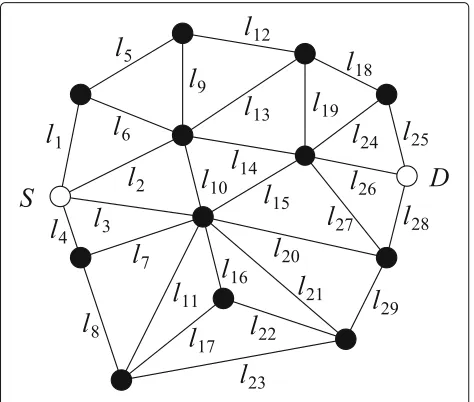
To guarantee the repeatability of simulation experiments, we will use the network with Q = 14 and J = 29 for performance evaluation, which is shown in Fig. 4. This network is generated according to the random graph the-ory [34], where the degree of the node is adjusted to be more than 2 for satisfying 1-identifiability, and the most left and most right nodes are selected asSandD, respec-tively. In addition, according to the method proposed in [7], 15 routes between S andDare selected, which are summarized in Table1. Note that we have the relation-ships amongQ,J, andIasQ ≈ J/2 andI ≈ J/2 for the network in Fig.4.

Furthermore, since the size of the network in Fig. 4 is limited, we will use other networks with larger sizes, which are also generated according to the same method for the one in Fig.4. Here, the performance depends on

J rather thanQ, so we will show the performance as the

Fig. 4Network withQ=14 andJ=29

Table 1Sets of routes

|Li| Li(i=1, 2,· · ·, 15)

3 L1= {l3,l15,l26},L2= {l2,l14,l26}

4 L3= {l4,l7,l20,l28}

5 L4= {l3,l16,l22,l29,l28},L5= {l2,l14,l19,l18,l25}, L6= {l2,l13,l18,l24,l26},L7= {l2,l10,l21,l29,l28}, L8= {l1,l5,l12,l18,l25}

6 L9= {l4,l8,l17,l16,l15,l26}, L10= {l4,l7,l21,l29,l27,l26}, L11= {l2,l9,l12,l19,l27,l28} 7 L12= {l3,l11,l23,l29,l27,l24,l25},

L13= {l1,l5,l9,l10,l20,l27,l26} 9 L14= {l1,l6,l14,l15,l11,l17,l22,l29,l28}

10 L15= {l4,l8,l23,l22,l16,l10,l13,l19,l24,l25}

function of J as the dependency on the network size, where we try to keep the relationships amongQ,J, andI

similar to those for the network in Fig.4.

In the simulation experiments, after settingηN =15 msec, σN = 3 msec [35, 36], and dev = 40 ppm [30, 31],

we selected K abnormal links out of 29 links randomly and evaluated the five schemes in 1000 tomography ses-sions. For each givenK, all combinations for the locations of abnormal links were realized, so the total tomogra-phy sessions resulted in29CK×1000. The thresholdθ in

(11) is set to 0.1, and the adjustable parameterξ in1/2

optimization is optimized.

For the evaluation, we define two metrics [37] to quan-tify two different types of errors that can occur in our identification problem. The first type of error corresponds to the case where normal links are falsely identified as abnormal links, and we refer to such errors as false pos-itives. We quantify the number of these errors using the false positive rate (FPR) defined (erroneous identification rate) as

FPR

ˆ

EA₌

EˆA_\EA

EˆA (101)

where EˆA _{is the set of the links identified to be}

abnor-mal links, andEAis the set of the actual abnormal links. On the other hand, the second type of error occurs when the abnormal links are not identified correctly. We refer to these errors as false negatives, and we quantify the num-ber of these errors using the false negative rate (FNR) defined (unidentified error rate) as

FNR

ˆ

EA₌

EA_{\ ˆE}A

We can evaluate a tomography scheme to be accurate if its errors in terms of the above two performance met-rics are suitably small. Especially when both the FPR and FNR equal zero, we can say that a perfect identifica-tion is accomplished, defining perfect identificaidentifica-tion ratio (PIR) as the ratio of the number of perfect identifications divided by the number of tomography sessions.

We will show the performance of the following five delay tomography schemes by simulation experiments; we refer to the subtractive delay tomography schemes with and without the route ordering in Section 5.4 as “Mid-Ave/Sub” and “Rand/Sub,” respectively, the differ-ential delay tomography schemes with and without (90) as “Order/Diff ” and “Rand/Diff,” respectively, and further-more, the conventional delay tomography scheme assum-ing a perfect clock synchronization betweenSandDonly at the beginning of the tomography session as “Conv.” If we can select aJ×Jfull-rank matrixBfor (37), we can per-form the non-compressed sensing-based abnormal link identification. However, noJ×J full-rank matrix always exists for a given network. In fact, for the network with

Q=14 andJ=29 in Fig.4, we can construct no 29×29 full-rank matrix.

8 Result and discussion

Figure5a,b, andcshow the dependencies of the PIR, FPR and FNR on the value of abnormal link delay (ηA),

respec-tively, for the network in Fig.4withTprobe=10 s andK =1.

We can see from these figures that the Conv scheme does not work well at all for smaller abnormal link delays due to the normal link delays and clock skew, even though perfect clock synchronization has been accomplished at the beginning of the tomography session. On the other hand, the Sub and Diff schemes have better performances than Conv scheme. The route ordering is effective for both schemes. In particular, the Order/Diff scheme out-performs the other four schemes in all the range ofηAand

especially when ηA is larger than 150 msec, which

cor-responds to be larger than around ten times the normal link delay (ηN = 15 msec), it can perfectly identify the

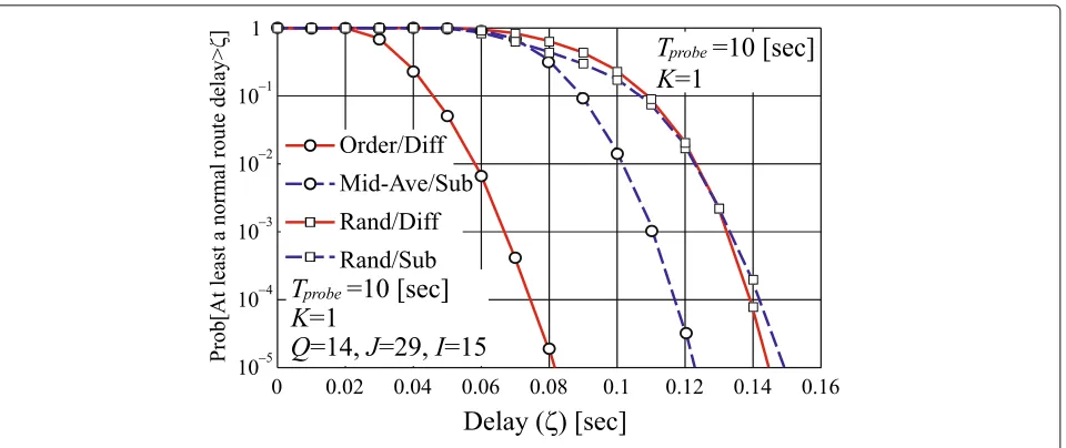
abnormal link. The performance of the Rand/Diff scheme is worse than the Sub schemes, especially for the smaller values of abnormal link delay. Let us discuss the reason for the phenomenon by an additional simulation experiment. SinceT_probe = 10 s in these figures, the magnitude of the clock skew is still less than 1 msec (= | _skT_probe| <

80×10−6_{×10= 0.8×10}−3_{), whereas that of the total}

normal link delays on a route is in the order of several tens of milliseconds from the system assumption. Therefore, the dominant source in es or ed can be the Gaussian-distributed normal link delays. If an abnormal link delay is much small, that is,x≈0, we haveys≈usoryd ≈ud. A false positive error occurs when the delay over at least one route which can be composed of only normal links reaches

a

b

c

Fig. 5Dependency on the abnormal link delay.aPIR,bFPR, andcFNR

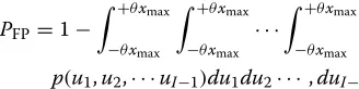
the identification threshold θxmax, so its probability is

given by

PFP=1−

( _+θxmax

−θxmax

( _+θxmax

−θxmax

· · ·

( _+θxmax

−θxmax

p(u1,u2,· · ·uI−1)du1du2· · ·,duI−1

(103)

wherep(u1,u2,· · ·,uI−1)is the joint probability density

function (pdf ) of u1,u2,· · ·, uI−1. Figure 6 shows the

Fig. 6Probability that a false positive error occurs

delay exceeds the delayζ seconds under the above condi-tion. From this figure, we can see that, forζ <0.13 s, the route delay for the Rand/Diff scheme exceedsζ more fre-quently than that for the Sub schemes, which meansPs_FP< P_FPd resulting in the superiority of the Sub schemes over the Rand/Diff scheme for the smaller values of abnormal link delay in Fig.5a.

Figure7a,b, andcshows the dependencies of the PIR, FPR, and FNR on the probing packet transmission inter-val (Tprobe), respectively, for the network in Fig. 4 with ηA = 1.0 s and K = 1. dev is extremely small

in the practical setting, so both Sub and Diff schemes are insensitive to the clock skew caused by dev when

Tprobe is smaller. However, these figures indicate the

superiority of the Diff schemes; the Diff schemes can perfectly identify the abnormal link keeping the FPR and FNR to zero even for larger Tprobe such as more

than 1000 s, while the Sub schemes incorrectly iden-tify an abnormal link when T_probe reaches around 300 s since the mismatch of clock frequency between S and

D keeps giving monotonously increasing bias to the route delay measurements during the tomography ses-sion. Furthermore, the Rand/Sub scheme corresponds to the one proposed in [13], so comparing the perfor-mances between the Rand/Sub and Mid-Ave/Sub schemes in Figs. 5 and 7, respectively, we can see that the route ordering/selection improves the performance of the Sub scheme.

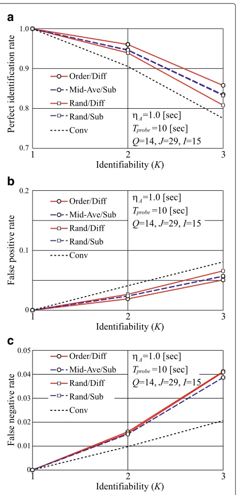
The routes were selected to be 1-identifiable, but Fig.8a, b, andcshows the dependencies of the PIR, FIR, and FNR on the identifiability (K), respectively, for the network in Fig.4withTprobe= 10sandηA=1.0 s. It is natural that

in Fig.8a, the PIRs of all the five schemes are one atK=1 and then they decrease asKincreases. The Sub schemes o

utperform the Rand/Diff scheme. Figure8bandcshows that the FPR dominates the degradation of the PIR, so this phe-nomenon comes from the same reason as that observed for the Sub schemes in Fig.5a, namely, the Diff schemes increase the probability that the delay of at least one nor-mal route exceeds the identification threshold. However, the most important fact is that the Order/Diff scheme shows the best performance.

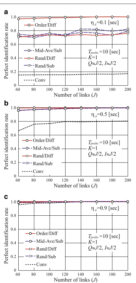
Figure9a,b, andcshows the dependencies of the PIR on the network size, assumingTprobe = 10 s andK = 1

forηA=0.1 s,ηA=0.5 s andηA=0.9 s, respectively. In

all the three figures, asJincreases, the PIRs tend to gradu-ally improve to 1.0, which means that larger size networks are more advantageous in terms of abnormal link iden-tifiability. This is because larger-size networks give more information on the single abnormal link through more dif-ferent measurement routes. It is obvious to see that the PIR more improves for largerηAfor all the five schemes,

but the superiority of the Order/Diff Scheme is outstand-ing; it can keep the PIR closer to 1.0 even for smallerηAin

smaller-size networks.

a

b

c

Fig. 7Dependency on the probing packet transmission interval. aPIR,bFPR, andcFNR

is important to note that the route ordering can be exe-cuted only once in an off-line manner before tomography session.

9 Conclusions

This paper proposed two kinds of synchronization-free delay tomography such as subtractive and differential schemes. We theoretically derived the optimal route refer-ence and ordering methods for the two schemes and then confirmed their robustness against clock asynchronism,

a

b

c

Fig. 8Dependency on the identifiability.aPIR,bFPR, andcFNR

a

b

c

Fig. 9Dependency on the network size.aηA=0.1,bηA=0.5, and cηA=0.9

Table 2Computational complexity

Scheme Route ordering Route delay subtraction

Conventional – –

Rand/Sub – O(I)

Mid-Ave/Sub O(I) O(I)

Rand/Diff – O(I)

Order/Diff OI2 O(I)

highest robustness against the clock asynchronism, clock skew, and normal link delays. The differential scheme can keep its identification accuracy even for much longer transmission interval of probing packet, so it is much harmless to normal sensor data traffic.

Compressed sensing-based delay tomography scheme is applicable for networks where non-compressed sensing-based scheme does not work, and it can identify abnormal links more accurately for larger-size networks. These two facts are its main advantages.

We have discussed the proposed schemes in a simple scenario, but we expect that they will be feasible in other scenarios such as passive proving strategy or where mul-tiple source and destination nodes are selected. We leave the application to other scenarios and real-world trace to verify the proposed schemes as our future works.

Endnote

1_{We intentionally useG=(N,L)instead ofG=(V,E)}

because we call the elements not “vertex” and “edge” but “node” and “link,” respectively, in this paper.

Appendix 1: Proof of Theorem 2

Define the subtractive routing matrices using the m1th

and m2th route references are B(m1) andB(m2),

respec-tively. When B(m1) _{is K-identifiable, SparkB}(m1) =

1 > 2K. Now, Spark

B(m1) = _{1 implies that the} smallest number of column vectors ofB(m1) _is1which are linearly dependent, so picking up different1column

vectors arbitrarily out of theJ−1 column vectors ofB(m1) asb(m1)

1 ,b

(m1)

2 ,· · ·,b

(m1)

q ,· · ·,b(m₁1)and a nonzero vector

asη= η1,η2,· · ·,ηq,· · ·,η1

, the following equation is satisfied:

b(m1)

1 ,b(2m1),· · ·,bq(m1),· · ·,b(m11)

η=0. (104)

Applying the fundamental manipulation on the addition of equations to (104), it can be converted to

⇒ b(m2)

1 ,b

(m2)

2 ,· · ·,b(qm2),· · ·,b(m12)

η=0 (105)

whereb(m2)

1 ,b(

m2)

2 ,· · ·,b(

m2)

q ,· · ·,b(m₁2)correspond to the

column vectors ofB(m2)_{. Conversely, we can derive}

b(m2)

1 ,b

(m2)

2 ,· · ·,b(qm2),· · ·,b(m22)

η = 0 (106)

⇒b(m1)

1 ,b(

m1)

2 ,· · ·,b(qm1),· · ·,b(m21)

η = 0. (107)

Appendix 2: Proof of Theorem 3

In this case, there is no guarantee that the abnormal links are correctly identified. However, applying the fun-damental manipulation on the subtractive matrix/vector equations, we have

y(m1)=_B(m1)_x⇔_y(m2)=_B(m2)_{x (108)}

that is, a set of solutions in selecting them1th route as the

reference is equivalent to that in selecting them2th route

as the reference.

Funding

This work was supported in part by the Japanese Ministry of Internal Affairs and Communications in R&D on Cooperative Technologies and Frequency Sharing Between Unmanned Aircraft Systems (UAS) Based Wireless Relay Systems and Terrestrial Networks, and JSPS KAKENHI grant numbers JP16K00124, and 18H01445.

Authors’ contributions

KN, SH, and TM contributed to the main idea and analyzed the results. KN and TN designed and carried out the simulation. KT, FO, and RM encouraged this whole work. All authors read and approved the final manuscript.

Competing interests

The authors declare that they have no competing interests.

Publisher’s Note

Springer Nature remains neutral with regard to jurisdictional claims in published maps and institutional affiliations.

Author details

1_{Wireless System Laboratory, Corporate Research & Development Center,}

Toshiba Corp., 212-8582 Kanagawa, Japan.2_{Graduate School of Engineering,} Osaka City University, 558-8585 Osaka, Japan.3Graduate School of Systems Design, Tokyo Metropolitan University, 191-0065 Tokyo, Japan.4_National Institute of Information and Communications Technology (NICT), 239-0847 Kanagawa, Japan.

Received: 4 February 2018 Accepted: 8 August 2018

References

1. M. H. Bhuyan, D. K. Bhattacharyya, J. K. Kalita, Network anomaly detection: methods, systems and tools. IEEE Commun. Surveys Tuts.16(1), 303–336 (2014)

2. J. N. Al-Karakim, A. E. Kamal, Routing techniques in wireless sensor networks: a survey. IEEE Trans. Wireless Commun.11(6), 6–28 (2004) 3. R. Castro, M. Coates, G. Liang, R. Nowak, B. Yu, Network tomography:

recent developments. Statist. Sci.19(3), 499–517 (2004)

4. M. Coates, A. O. Hero III, R. Nowak, B. Yu, Internet tomography. IEEE Signal Process. Mag.19(3), 47–65 (2002)

5. Y. Vardi, Network tomography: estimating source-destination traffic intensities from link data. J. Amer. Stat. Assoc.91(433), 365–377 (1996) 6. M. H. Firooz, S. Roy, Link delay estimation via expander graphs. IEEE Trans.

Commun.62(1), 170–181 (2014)

7. K. Takemoto, T. Matsuda, T. Takine, Sequential loss tomography using compressed sensing. IEICE Trans. Commun.E96-B(11), 2756–2765 (2013) 8. W. Xu, A. Tang, inProc. 48th Annu. Allerton Conf. Commun., Control,

Comput.: 29 Sept.-1 Oct. 2010. Compressive sensing over graphs: how many measurements are needed? (IEEE, Allerton, 2010), pp. 16–27 9. D. L. Donoho, Compressed sensing. IEEE Trans. Inf. Theory.52(4),

1289–1306 (2006)

10. Y. C. Eldar, G. Kutyniok,Compressed sensing: theory to applications. (Cambridge University Press, Cambridge, 2012)

11. J. Zhao, R. Govindan, D. Estrin, Sensor network tomography: monitoring wireless sensor networks. ACM SIGCOMM Comput. Commun. Rev.32(1), 64–64 (2002)

12. G. Hartl, B. Li, inProc. 3rd IPSN: 26 - 27 Apr. 2004. Loss inference in wireless sensor networks based on data aggregation (IEEE, Berkeley, 2004), pp. 396–404

13. K. Nakanishi, S. Hara, T. Matsuda, K. Takizawa, F. Ono, R. Miura, Synchronization-free delay tomography based on compressed sensing. IEEE Commun. Lett.18(8), 1343–1346 (2014)

14. K. Nakanishi, S. Hara, T. Matsuda, K. Takizawa, F. Ono, R. Miura, Reflective network tomography based on compressed sensing. Procedia Computer Science.52, 186–193 (2015)

15. T. Naka, S. Hara, Route selection algorithms utilizing the property of the ZDD for compressed sensing-based transmissive network tomography. Procedia Comput. Sci.109, 124–131 (2017)

16. I. F. Akyildiz, X. Wang, W. Wang, Wireless mesh networks: a survey. Comput. Netw.47(4), 445–487 (2005)

17. B. Sundararaman, U. Buy, A. D. Kshemkalyani, Clock synchronization for wireless sensor networks: a survey. Ad Hoc Netw.3(3), 281–323 (2005) 18. E. D. Kaplan, C. J. Hegarty,Understanding GPSP: principles and applications,

Second Edition. (Artech House, Norwood, 2012)

19. D. L. Mills, Internet time synchronization: the network time protocol. IEEE Trans. Commun.39(10), 1482–1493 (1991)

20. S. Ganeriwal, R. Kumar, M. B. Srivastava, inProc. First Int. Conf. Embedded Networked Sensor Syst.: 5–9 Nov.Timing-sync protocol for sensor networks (ACM, New York, 2003), pp. 138–149

21. K. Noh, E. Serpedin, inProc. IEEE Int. Symp. World Wirel., Mob. Multimedia Netw.: 18–21 June; Espoo. Pairwise broadcast clock synchronization for wireless sensor networks, (2007), pp. 1–6

22. Y. Zhang, T. Qiu, L. Liu, Y. Sun, A. Zhao, F. Xia, inProc. ICSN 2016: 23–26 May. Mac-time-stamping-based high-accuracy time synchronization for wireless sensor networks (IEEE, Jeju, 2016), pp. 1–4

23. V. F. Kroupa,Frequency stability: introduction and applications. (Wiley, Hoboken, 2012)

24. T Otsuka, S. Hara, T. Matsuda, K. Takizawa, F. Ono, R. Miura, inProc. WPMC 2015: 13–16 Dec. 2015. Path ordering and reference selection method for the differential delay tomography (IEEE, Hyderabad, 2015). in CD-ROM 25. M. Elad,Sparse and redundant representations: from theory to applications in

signal and image processing. (Springer, New York, 2010)

26. M. Zibulevski, M. Elad, L1-l2 optimization in signal and image processing. IEEE Signal Process. Mag.27(3), 76–88 (2010)

27. T. Matsuda, M. Nagahara, K. Hayashi, Link quality classifier with compressed sensing based on1-2optimization. IEEE Commun. Lett. 15(10), 1117–1119 (2011)

28. A. Beck, M. Teboulle, A fast iterative shrinkage-thresholding algorithm for linear inverse problems. SIAM J. Imaging Sci.2(1), 183–202 (2009) 29. D. Johnson, Y. Hu, D. Maltz,RFC: 4728, The dynamic source routing protocol

(DSR) for mobile ad hoc networks for IPv4. (IETF, Fremont, 2007) 30. IEEE: Std 802.11–2012 - Wireless LAN medium access control (MAC) and

physical layer (PHY) specifications (2012)

31. IEEE: Std 802.15.4–2011 - Low-rate wireless personal area networks (LR-WPANs) (2011)

32. K. L. Noh, Q. M. Chaudhari, E. Serpedin, B. W. Suter, Novel clock phase offset and skew estimation using two-way timing message exchanges for wireless sensor networks. IEEE Trans. Commun.55(4), 766–777 (2007) 33. G. P. Agrawal,Fiber-optic communication systems. (John Wiley & Sons,

Hoboken, 2010)

34. B. Bollobas,Random graphs, 2nd Ed. (Cambridge Univ. Press, Cambridge, 2001)

35. W. Zeng, X. Chen, X. Kim, Z. Bu, W. Wei, B. Wang, Z. J. Shi, inProc. IEEE MILCOM.: 18–21 Oct. 2009. Delay monitoring for wireless sensor networks: an architecture using air sniffers (IEEE, Boston, 2009), pp. 1–8

36. K. Liu, Q. Ma, H. Liu, Z. Cao, Y. Liu, inProc. IEEE MASS: 14–16 Oct. 2013. End-to-end delay measurement in wireless sensor networks without synchronization (IEEE, Hangzhou, 2013), pp. 583–591