Modified Kernel Functions by Geodesic Distance

Modified Kernel Functions by Geodesic Distance

Quan Yong

Institute of Image Processing & Pattern Recognition, Shanghai Jiaotong University, Shanghai 200030, China Email:[email protected]

Yang Jie

Institute of Image Processing & Pattern Recognition, Shanghai Jiaotong University, Shanghai 200030, China Email:[email protected]

Received 20 August 2003; Revised 9 March 2004

When dealing with pattern recognition problems one encounters different types of prior knowledge. It is important to incorporate such knowledge into the classification method at hand. A common prior knowledge is that many datasets are on some kinds of manifolds. Distance-based classification methods can make use of this by a modified distance measure called geodesic distance. We introduce a new kind of kernels for a support vector machine (SVM) which incorporates geodesic distance and therefore is applicable in cases where such transformation invariance is known. Experiments results show that the performance of our method is comparable to that of other state-of-the-art methods, such as SVM-based Euclidean distance.

Keywords and phrases:support vector machine, geodesic distance, kernel function.

1. INTRODUCTION

Support vector machine (SVM) is a new promising pattern classification technique proposed recently by Vapnik and coworkers [1,2]. Unlike traditional methods which mini-mize the empirical training error, SVM aims at minimizing an upper bound of the generalization error through control-ling the margin between the separating hyperplane and the data. This can be regarded as an approximate implemen-tation of the structure risk minimization principle. What makes SVM attractive is the property of condensing infor-mation in the training data and providing a sparse represen-tation by using a very small number of data points.

SVM is a linear classifier in the parameter space, but it is easily extended to a nonlinear classifier of theφ-machine type by mapping the spaceS = {x}of the input data into a high-dimensional feature space F = {φ(x)}. By choos-ing an appropriate mappchoos-ingφ, the data points become lin-early separable or nlin-early linlin-early separable in the high-dimensional space so that one can easily apply the struc-ture risk minimization. Instead of computing the mapped patternsφ(x) explicitly, we only need the dot products be-tween the mapped patterns. They are directly available from the kernel function which integratesφ(x). By choosing dif-ferent kinds of kernels, the SVM can realize radial basis func-tion (RBF) and polynomial and multilayer perceptron clas-sifiers. Compared with the traditional way of implementing them, the SVM has an extra advantage of automatic model selection, in the sense that both the optimal number and the

locations of the basis functions are automatically obtained during training.

Like neural networks, SVM also uses a distance function to determine how close an input vector xis to each stored data [3]. As mentioned in [4], a variety of distance functions are available for such use, including the Minkowski, Ma-halanobis, Camberra, Chebychev, and Chi-square distance metrics. Although there have been many distance functions proposed, by far the most commonly used is the Minkowski distance. Euclidean distance is the most special case of the Minkowski distance. The choice of distance function influ-ences the bias of a learning algorithm. A bias is a rule or method that causes an algorithm to choose one generalized output over another. A learning algorithm must have a bias in order to generalize, and it has been shown that no learning al-gorithm can generalize more accurately than any other when summed over all possible problems [5]. It follows then that no distance function can be strictly better than any other in terms of generalization ability, when considering all possible problems with equal probability. So, an appropriate distance function should be selected according to datasets. Especially for those data points which lie in a manifold, Euclidean dis-tance cannot reflect the real disdis-tance between two points.

In this paper, we focus on the design of SVM based on the geodesic distance. We first propose an improved geodesic distance to eliminate isolated embeddings, then the geodesic distance is applied to the kernel of SVM. Experiments show that good generalization can be obtained using the revised SVM.

2. MINKOWSKI METRIC AND ITS LIMITATIONS

The Minkowski metric [7] is widely used for measuring sim-ilarity between points. Suppose two pointsxandyare rep-resented by two p dimensional vectors (x1,x2,. . .,xp) and

wherer is the Minkowski factor for the norm. Particularly, whenr is set as 2, it is the well-known Euclidean distance; whenr is 1, it is the Manhattan distance (orL1distance). A point located a smaller distance from a query point is deemed more similar to the query point. Measuring similarity by the Minkowski metric is based on one assumption: the similar point should be close to the query point in all dimensions.

A variant of the Minkowski function, the weighted Minkowski distance function, has also been applied to mea-sure the point similarity. The basic idea is to introduce weighting to identify important features. By assigning each feature a weighting coefficientwi(i=1,. . .,p), the weighted Minkowski distance function is defined as

dw(x,y)=

By applying a static weighting vector for measuring sim-ilarity, the weighted Minkowski distance function assumes that similar points resemble the query points in the same fea-tures. However, in some cases, Minkowski distance does not reflect the geodesic distance between two points.Figure 1 il-lustrates how Euclidean distance exploits the distance for two points on a manifold.

AsFigure 1shows, for two arbitrary points (circled) on a nonlinear manifold, their Euclidean distance in the high-dimensional input space (length of dashed line) may not ac-curately reflect their geodesic distance, as illustrated by the solid curve.

3. REVISED GEODESIC DISTANCE

3.1. Constructing the geodesic distance path

Tenenbaum proposed a new algorithm for estimating geo-desic distances. The basic idea is that for a neighborhood of points on a manifold, the Euclidean distances provide a fair approximation of geodesic distance. For faraway points the geodesic distance is estimated by the length of the shortest path through neighboring points.

Figure1: Distance between two points on a manifold.

a

Figure2: Inaccuracy of Euclidean distance compared with geodesic distance.

Leta,b, andcbe given samples from a manifold struc-ture. One does not assume to know the true manifold which would be the curve in this example (see Figure 2). The geodesic distancesgabandgbc would be measured along the manifold, while dab,dbc, anddac denote the Euclidean dis-tance. When describing relations between the points, the aim is to take the assumed manifold structure into considera-tion. Therefore, one tries to estimate the geodesic distance for a given set of points. As one can see for this example, the geodesic distance between neighboring points can be ap-proximated fairly well by their Euclidean distances, so that

gab = dab andgbc = dbc. The geodesic distance betweena andcwould begac=gab+gbcfor whichgac =dab+dbcis a far better approximation thandac. So, for neighboring points the geodesic distance is approximated by Euclidean distances and for distant points one considers the length of the shortest path through neighboring points.

1

0.5

0

−0.5

−1

−1 −0.5 0 0.5 1

(a)

1

0.5

0

−0.5

−1

−1 −0.5 0 0.5 1

(b)

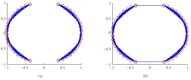
Figure3: Shortest paths on manifold.

points lie on a submanifold of Rn_{. In a first step, the} Eu-clidean distance matrixDi j =d(xi,xj) is computed and for eachxi ∈Xa set of neighboring pointsZ(xi) is determined by

Zxi =xj|xj∈Xis neighbor ofxj

. (3)

Several variants for defining neighborhood relations can be used, for example,k-nearest neighbors,ε-ball neighbor-hood. These relations are used to construct the undirected neighborhood path, which will be represented by an (m×m) adjacency matrix G. The adjacency matrix G is initialized with connections between neighbors, weighted by their Eu-clidean distance

Gi j=   d

xi,xj ifi∈Zxj or j∈Zxi ,

∞ ifxiandxjare not neighbored, (4)

where∞just denotes that two points are not connected. In this paper, we adopt thek-nearest neighbor algorithm to de-termine which points are neighbors on the manifold. Since the graph is undirected, the adjacency matrix has to be sym-metrizedGi j =min(Gi j,Gji), which clarifies the symmetry of the neighborhood relation.

In the second step, the geodesic distances for not directly connected points are estimated by the length of the shortest path inGbetween them. Computationally, this is a standard all-pairs-shortest-path problem for which several algorithms are available. In this paper, a Floyd-Warshall algorithm will be used. If we apply the algorithm toG, the resulting value of Gi jis the length of the shortest path and so the approximated geodesic distance between the vertices representingxiandxj, if such a path exists.

The accuracy of the estimated intrinsic geometry natu-rally depends on the density of the samples, errors in the data relative to the manifold, the smoothness of the manifold, and the way the neighborhood graph is constructed.

3.2. Connecting subgraphs

Problems arise when the graph is not connected, which can be a result of noncontinuous sampling, an inadequate con-struction of neighborhoods or structural breaks in the data. In that case, the construction of neighborhoods has to be modified or additional connections have to be made un-til the all-pairs-shortest-path procedure gives a connected graph adjacency matrix (∀i,j :Gi j = ∞), which then is the matrix of estimated geodesic distance.

Figure 3ashows that the resulting graph is unconnected. In this situation, Tenenbaum chooses only the largest com-ponent for embedding. This method works only when the largest component covers most of the training samples. Since this would imply that the remaining points would be dis-carded, this alternative will loose part of information. When the number of points that each subgraph contains is nearly equal, the largest component cannot substitute for the whole sample space. So, errors may occur. In this paper, we choose to link the subgraphs and take all points into consideration.

To link the subgraphs algorithmically, the simplest method to ensure the connectedness is the “single link-age” method. Suppose xi and xj are in two unconnected subgraphs, respectively, which show the smallest Euclidean distanceDi jamong all unconnected points, we link the two points. Their connection can be penalized by enlarging the corresponding length inG. For example, in this paper, we set its lengthLi j in proportion toDi j and the maximal valueg in every subgraph. Then we have to update the distance in G. Note that this does not require a full run of an all-pairs-shortest-path procedure, since if two points are newly con-nected, the shortest path between them must include the new connection betweenxiandxj. Thus, for all pairsxa,xbof pre-viously unconnected points we have to compute

Gab=minGai+Li j+Gjb,Ga j+Li j+Gib . (5)

3.3. Supervised geodesic distance

Until now, geodesic distance has been used as an unsuper-vised technique. However, we can take the classification in-formation into consideration. The geodesic distance prob-lem can easily be rephrased to use class label information, ωi ∈ Ω(|Ω| = c) with eachxi, during training. The idea is to find a mapping separating within-class structure from between-class structure. The easiest way to do this is to select the neighbors from just the class thatxiitself belongs to.

A slightly more complicated method would be by using the distance matrix formulation as in (5), but adding dis-tance between samples in different classes:

G=G+µmax(G)∆, (6)

where∆jm=1 ifωj=ωm, and 0 otherwise. In this formula-tion,µ∈[0, 1] controls the amount to which the class infor-mation should be incorporated. A dataset is created in which there arec“disconnected” classes, each of which should be connected fairly by geodesic distance. These added degrees of freedom are used to separate the classes.

4. TRAINING SVM WITH GEODESIC DISTANCE

SVMs [8] are a general class of learning architecture inspired from the statistical learning theory that performs structural risk minimization on a nested set structure of separating hy-perplanes. Given a training data, the SVM training algorithm obtains the optimal separating hyperplane in terms of gener-alization error.

The support vector algorithm

Suppose we are given a set of examplesx1,y1),. . ., (xl,yl)∈

RN_{. yi ∈ {−1, +1}. We consider functions of the form} sgn((w·x) +b). In addition, we impose the condition

inf i=1,...,l

_{w·xi +b=1. (7)}

We would like to find a decision function fw,b with the properties fw,b(xi)= yi;i =1,. . .,l. If this function exists, condition (7) implies

yiw·xi +b ≥1, i=1,. . .,l. (8)

In many practical situations, a separating hyperplane does not exist. To allow for possibilities violating equation (8), slack variables are introduced:

ξi≥0, to getyiw·xi +b ≥1−ξi, i=1,. . .,l. (9)

The support vector approaches to minimize the general-ization error consists of the following. Minimize

Φ(w,ξ)=(w·w) +γ l

i=1

ξi (10)

subject to the constraints (9).

It can be shown that minimizing the first term in (10) amounts to minimizing the VC-dimension, and minimizing the second term corresponds to minimizing the misclassifi-cation error [8]. The minimization problem can be posed as a constrained quadratic programming (QP) problem. The so-lution gives rise to a decision function of the form

f(x)=sgn

Only a small fraction of theaicoefficients is nonzero. The corresponding pairs ofxientries are known as support tors and fully define the decision function. The support vec-tors are geometrically the points lying near the class bound-aries. We use linear kernels for SVM, nonlinear kernels may also be used.

4.1. Geodesic distance for kernel functions

Kernel functions are used in SVM. A possible interpretation of their effects is that they represent dot products in some feature spaceF, that is,

kxi,xj =φ

xi ·φxj , (12)

whereφis a map from input (data) spaceXintoF. Another interpretation is to connectφwith the regularization prop-erties of the corresponding learning algorithm. These expen-sive calculations can be reduced significantly by using a suit-able functionk, leading to decision functions of the form

f(x)=sgn

Most popular kernels are translation invariant kernels

kxi,xj =k

xi−xj . (14)

Usually, the translation invariant kernels can be ex-pressed ask(xi,xj)= f(d(xi,xj)). Then the distancesDcan be used to compute a feature space Gram matrix by Ki j = f(Di j). Compared with Euclidean distance, the geodesic dis-tance reflects the true disdis-tance. In this paper, we use the geodesic distance to measure similarity. Thus, kernel func-tion becomesKi j = f(Gi j). In the experiments, RBF kernel is taken. So,

LetGlbe the matrix of estimated geodesic distances com-puted fromXl. The geodesic distances of the instancext to-wards all points inXlcan be estimated as follows. First, the (m×1) vectordtof Euclidean distances between the rest ob-servationxtand the points in the training setXlis calculated. Then, the neighborhoodZ(xt) ofxtis determined using the same neighborhood rule as was used for the initialization of Gl. So, the geodesic distance betweenxt andxi can be esti-mated by

gxt,xi = min j:xj∈Z

Gi j+dxj,xt . (16)

4.3. Computational complexity

What makes geodesic distance algorithm more practical in terms of processing time is that it can be optimized us-ing Dijkstra’s algorithm for computation of shortest paths in a graph. Compared to Euclidean distance, the standard geodesic distance algorithm tends to have more computa-tional complexity. One has to calculate the l×l shortest-path distance matrix Gl. The simplest way is Floyd’s algo-rithm with complexityO(l3_{). Dijkstra’s algorithm is very} sig-nificant, because this optimization reduces the processing time from the order of hours to the order of minutes, even to seconds. Such a reduction in time is explainable by ob-serving that the time complexity for Dijkstra’s algorithm is O(llogl+E), where l is the number of vertices andE is the number of edges. For meshes with O(103_{) vertices,} ex-act geodesics can be computed in about 25 seconds on a 633 MHz Celeron II PC.

Moreover, training an SVM requires the solution of a very large QP optimization problem. For datasets ofO(103₎ sam-ples, it will take nearly 163 seconds to solve the QP problem. So, the computational time of geodesic distance has a small part in the whole training time of SVM. Once the training process is finished, the SVM can be used in online classifica-tion tasks. One will have to compute the geodesic distances of a testing sample to all of the training samples. Instead of recomputing the geodesic distance matrix,Section 4.2 intro-duces a new method to solve this problem and speeds the computation greatly.

5. NUMERICAL RESULTS AND COMPARISONS

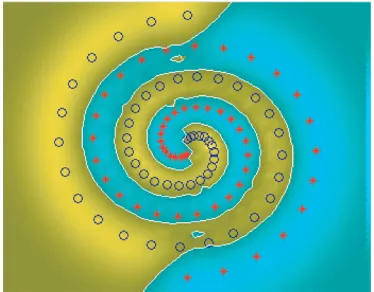
Experiment1 (a two-spiral problem). The two-spiral

prob-lem [9] is a well-known benchmark problem for testing the quality of neural network classifiers. In this experiment (Figure 4), we illustrate an using modified geodesic distance on a two-spiral problem. The training data are shown on

Figure 4 with two classes indicated by “” and “∗” (100 points with 50 for each class) in a two dimensional input space. Points in between the training data located on the two spirals are often considered as test data for this problem, but are not shown on the figure. The excellent generalization per-formance is clear from the decision boundaries shown on the figure. In this case,δ=1 andγ=10 were chosen as param-eters. This experiment shows that the SVM using modified geodesic distance can work well on complex datasets.

Figure4: A two-spiral classification problem with the two classes indicated by “” and “∗.”

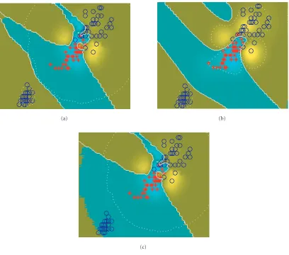
Experiment 2 (iris dataset problem). In the second

exper-iment, we compare the feature of the SVM using modi-fied geodesic distance proposed in this paper with the SVM using unmodified geodesic distance. Here, the unmodified geodesic distance means the geodesic distance implemented by Tenenbaum. The iris dataset problem [10] is also a well-known benchmark problem for testing the quality of neural network classifiers. In this experiment (Figure 5), we illus-trate the results of SVMs using modified geodesic distance (Figure 5a), unmodified geodesic distance (Figure 5b) and Euclidean distance (Figure 5c) on iris dataset problem. The training data are showing onFigure 5with two classes indi-cated by “” and “∗” in a two-dimensional input space. Like

Experiment 1, we take points in between the training data lo-cated on the plane as test data for this problem. In this case, δ=0.5 andγ=20 were chosen as parameters.

FromFigure 5bwe can see that many points are misclas-sified by the SVM using unmodified geodesic distance. For the iris dataset, there are two subgraphs when constructing geodesic distance path. The unmodified geodesic distance, implemented by Tenenbaum, is to choose only the largest subgraph for learning. So, only part of training examples is used, that is the reason why some important information contained in training examples may be lost. That leads to a disappointing result.

In our modified geodesic distance algorithm, we connect the subgraphs post. As a result, we take all training ex-amples into consideration when using SVM. FromFigure 5a

we can see that the SVM using modified geodesic distance can correctly classify the examples that is misclassified in

Figure 5b. This experiment shows that the SVM based on modified geodesic distance can take full advantage of all training examples and gain better classification results than that of the SVM based on unmodified geodesic distance.

From Figures 5a and 5c, we can see that when the structure of the training samples is simple, the SVM using modified geodesic distance can gain comparable results as that of the SVM using Euclidean distance. But when train-ing samples are in high-dimensional space, the structure is usually very complicated and the results are very different.

(a) (b)

(c)

Figure5: Iris dataset classification problem with the two classes indicated by “” and “∗.”

Experiment3 (real datasets). In order to compare the

classifi-cation accuracy of the SVM using modified geodesic distance proposed in this paper, the SVM using Euclidean distance on massive datasets, and the SVM using unmodified geodesic distance, we test this algorithm on three real-world datasets. Here, the proposed SVM means the SVM using modified geodesic distance proposed in this paper, the classical SVM means the SVM using Euclidean distance, and the geodesic SVM means the SVM using unmodified geodesic distance.

In this experiment, we adopt the same datasets used in [11], that is, we choose the Boston housing and the Abalone dataset from the UCI repository [Blake et al., 1998] and the USPS database of handwritten digits. The first data are of size 506 (350 training, 156 testing), the Abalone dataset of size 4177 (3000 training and 1177 test-ing). In the first two cases, the data were rescaled to zero mean and unit variance, coordinate-wise, while the USPS dataset remained unchanged. Its data size is 40337 (29463 training and 10874 testing). Finally, the gender en-coding in Abalone (male/female/infant) was mapped into {(1, 0, 0), (0, 1, 0), (0, 0, 1)}.

Table 1illustrates testing error rate, training set size, and the number of support vectors for classical SVM and the

pro-posed SVM algorithms. Here, we can see that in almost every dataset, the new proposed SVM can gain lower testing er-ror rate than the classical SVM and the geodesic SVM. When a dataset contains nonlinear structure, the geodesic distance reflects intrinsic relations in the data and contains proper-ties of the curvature of the manifold. Therefore, more prior knowledge about the training data is considered. Especially in large amount of datasets as shown inTable 1, the new pro-posed SVM can gain higher classification accuracy than that of the other two methods.

6. CONCLUSIONS

Table1: Comparison on various datasets.

Dataset SVM Classification_{accuracy (%)} Training

set size Number of SVs Training time (s)

SVM parameters

δ γ

Boston housing

Classical SVM 92.74±0.86 350 167±6 5.8±0.3 150 0.5

Geodesic SVM 93.26±0.47 350 153±4 6.3±0.2 150 0.5

Revised SVM 94.42±0.08 350 143±10 6.7±0.4 150 0.5

Classical SVM 87.44±1.01 3000 1317±15 378.8±13.1 500 20.0

Abalone Geodesic SVM 82.17±2.13 3000 932±26 307±21.6 500 20.0

Revised SVM 93.37±1.24 3000 1277±11 462.3±24.3 500 20.0

Classical SVM 91.1±0.64 29463 11533±5 8221.9±147.8 700 5.0

USPS Geodesic SVM 83.6±0.81 29463 9677±19 7994±152.4 700 5.0

Revised SVM 96.5±0.31 29463 9874±5 9186.3±276.4 700 5.0

ACKNOWLEDGMENTS

This work was Supported by the National Natural Science Foundation of China under Grant no. 50174038. The sec-ond author is now supported by the National Natural Science Foundation of China under Grant no. 30170274.

REFERENCES

[1] V. N. Vapnik, Statistical Learning Theory, John Wiley, New York, NY, USA, 1998.

[2] N. Cristianini and J. Shawe-Taylor,An Introduction to Support Vector Machines, Cambridge University Press, Cambridge, UK, 2000.

[3] B. Sch¨olkopf,Support Vector Learning, R. Oldenbourg Verlag, Munich, Germany, 1997.

[4] D. R. Wilson and T. R. Martinez, “Improved heterogeneous distance functions,” Journal of Artificial Intelligence Research, vol. 6, pp. 1–34, 1997.

[5] C. Schaffer, “A conservation law for generalization perfor-mance,” inProc. 11th International Conference on Machine Learning, pp. 259–265, Morgan Kaufmann, San Mateo, Calif, USA, 1994.

[6] J. B. Tenenbaum, V. D. Silva, and J. C. Langford, “A global ge-ometric framework for nonlinear dimensionality reduction,” Science, vol. 290, pp. 2319–2323, 2000.

[7] B. G. Batchelor,Pattern Recognition: Ideas in Practice, Plenum Press, New York, USA, 1978.

[8] C. J. C. Burges, “A tutorial on support vector machines,”Data Mining and Knowledge Discovery, vol. 2, no. 2, pp. 121–167, 1998.

[9] S. Ridella, S. Rovetta, and R. Zunino, “Circular back-propagation networks for classification,” IEEE Transactions on Neural Networks, vol. 8, no. 1, pp. 84–97, 1997.

[10] R. A. Fisher, “The use of multiple measurements in taxonomic problems,”Annals of Eugenics, vol. 7, no. 2, pp. 179–188, 1936. [11] A. J. Smola and B. Sch¨olkopf, “Sparse greedy matrix approxi-mation for machine learning,” inProc. 17th International Con-ference on Machine Learning, pp. 911–918, Morgan Kaufman, San Francisco, Calif, USA, 2000.

Quan Yong was born in Hei Longjiang province, China, in 1976. He received his B.S. and M.S. degrees in mechanical & elec-trical engineering from Harbin Institute of Technology, Harbin, China. Since 2000, he has been a Ph.D. candidate at the Institute of Image Processing and Pattern Recogni-tion, Shanghai Jiaotong University, China. His current research areas include machine learning and data mining.