Construction of a database for a dynamic CGE model for South Africa

(1)

Eleventh Floor, Menzies Building

Monash University, Wellington Road

C

LAYTON

Vic 3800 A

USTRALIA

Telephone:

from overseas:

(03) 9905 2398, (03) 9905 5112

61 3 9905 2398 or

61 3 9905 5112

Fax:

(03) 9905 2426

61 3 9905 2426

e-mail:

[email protected]

Internet home page:

http//www.monash.edu.au/policy/

Construction of a Database for a Dynamic

CGE Model for South Africa

by

L

OUISE

ROOS

Centre of Policy Studies

Monash University

General Paper No. G-234 May 2013

ISSN 1 031 9034

ISBN 978 1 921654 42 8

(2)

(3)

i

Construction of a database for a dynamic CGE model for South

Africa

Louise Roos

Centre of Policy Studies, Monash University, Australia, May 2013.

Abstract

This paper describes the construction of database constructed for a dynamic CGE model for South Africa (hereafter SAGE). The starting point for creating a database for a CGE model are official data from an Input/output (IO) table, or from a Supply Use Table (SUT), or from a Social Accounting Matrix (SAM). Often the structure of the published data is not in the required format of a CGE database, and so a major task is to transform the official data into a form required by a CGE database. Four characteristics of the SAGE database are noted:

1. It contains information regarding the structure of the South African economy in the base year (2002).

2. It is the initial solution to the SAGE model.

3. It has the same basic structure as the ORANIG and MONASH databases. 4. The basic database is supplemented by additional data relating to dynamics.

The database is organised in four parts. The first includes data on the coefficients that are computed from the input–output (IO) table. These coefficients represent the basic flows of commodities between users, commodity taxes paid by users, margin flows that facilitate the flow of commodities and valued added matrices. The second part of the SAGE database contains information on behavioural parameters. The elasticities influence the degree to which economic agents change their behaviour when relative prices change. The third part of the database contains information on government accounts, accounts with the rest of the world and industry-specific capital stocks and depreciation rates. The fourth part of this paper describes the tests undertaken to test for model validity.

This paper is set out as follows: Section 1 describes the structure of the IO database. Section 2 reviews the official data sources used to create the IO database. Section 3 describes the steps taken to transform the official data into the correct format. Section 4 describes the elasticities and parameters adopted in for SAGE. Section 5 describes additional information regarding industry-specific capital stocks and government accounts. Section 6 describes various tests that were conducted to ensure that the database is balanced. The paper ends with a conclusion.

Key words: Computable general equilibrium (CGE), Database, Africa, Supply Use Tables

(4)

(5)

iii

TABLE OF CONTENTS

LIST OF ABBREVIATIONS LIST OF SETS

LIST OF TABLES LIST OF FIGURES

1. Basic structure of a CGE database

1.1. Introduction……….……1

1.2. Parameters……….. 6

1.3. Data required for SAGE’s dynamic equations..……….……….… 6

2. Data sources……… 8

2.1. Note on the valuation of the tables……….……… 8

2.2. Basic structure of the Supply-Use Tables (2002) for South Africa……….. 8

2.2.1. The Supply table………. 9

2.2.2. The Use table……… 9

2.3. Other data sources………... 10

2.3.1. Social accounting matrix (2002)……… 10

2.3.2. South African Reserve Bank Quarterly Bulletin……….. 10

2.3.3. Government accounts………... 11

2.3.4. Use of GTAP data to specify land rents………... 11

2.3.5. Sector-specific data………..……. 11

3. Stages in the compilation of the SAGE database………. 11

3.1. Step 1: Data mapping and aggregation……….… 12

3.2. Step 2: Distribution of the residual……… 13

3.3. Step 3: Adjustments to the Supply and Use table………. 13

3.4. Step 4: Check that aggregate supply is equal to aggregate demand………... 15

3.5. Step 5: Creating land rentals………... 16

3.6. Step 6: Splitting flows into sources……….… 17

3.7. Step 7: Creating an Ownership of Dwellings commodity and industry……….. 18

3.7.1. Value of output……….….19

3.7.2. Sales structure……….… 19

3.7.3. Input structure……… 19

3.8. Step 8: Creating margin matrices……… 20

3.8.1. Calculation of aggregate margin matrices, by user………. 22

3.8.2. Creating margin matrices by type of margin commodity……….. 22

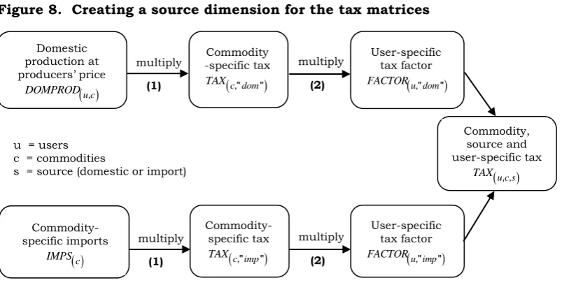
3.9. Step 9: Creating tax matrices……… 23

3.9.1. Defining the different taxes………. 23

3.9.2. Creating indirect tax matrices for all users……….……….. 25

3.9.3. Tax on production……….. 26

3.10. Step 10: Creating matrices for the basic flows……… 26

(6)

iv

3.11.1. Calculating industry-specific investment………..……… 27

3.11.1.1. Calculating industry-specific depreciation rates

 

d …….. 28

3.11.1.2. Calculating industry-specific capital growth rates

 

k ….. 30

3.11.1.3. Calculating industry-specific rates of return

 

R …………. 30

3.11.2. Completing the investment matrix………..…. 33

3.11.3. Determining industry-specific capital stocks………....33

3.12. Step 12: Final balancing of the SAGE database……….… 34

3.12.1. Condition 1: industry cost should equal industry output……….... 34

3.12.2. Condition 2: domestic commodity output equals domestic use…….… 34

4. Parameters and elasticities………..……….… 36

4.1. The substitution parameters between primary factors……….………….. 37

4.2. The CES substitution elasticities between labour occupations……….38

4.3. The elasticities of substitution between domestic and foreign sources of supply.. 38

4.4. The constant elasticity of transformation (CET elasticity)……….… 40

4.5. Export demand elasticities………..….. 40

4.6. The household expenditure and marginal budget shares……….…. 41

4.7. Frisch parameter……….. 42

5. Additional data required for the dynamic equations………. 43

5.1. Investment and capital stock……….……43

5.1.1. Difference between maximum and trend growth rate of capital………. 43

5.1.2. Real interest rate………. 43

5.1.3. Asset price of capital………..… 43

5.1.4. The average sensitivity of capital growth to changes in expected rates of return……….. 43

5.1.5. CPI and lagged CPI………. 43

5.2. Government accounts……….… 44

5.2.1. Revenue and expenditure items………. 44

5.2.2. Tax rates on labour and capital incomes……… 45

5.2.3. Transfers……… 46

5.2.4. Public sector debt and interest paid on public sector debt………...46

5.2.5. Government investment……… 46

5.3. Accounts with the rest of the world……… 46

5.3.1. Gross national product (GNP)………. 47

5.3.2. Foreign debt and the interest rate on foreign debt in the base year…. 47 5.3.3. Exchange rate……….. 47

6. Test for model validity……….. 47

6.1. Test 1: Real and nominal homogeneity tests……….. 47

6.2. Test 2: GDP from the income and expenditure side……….. 48

6.3. Test 3: Updated database should be balanced………... 48

6.4. Test 4: Repeat the above steps using a multi-step solution method……….. 48

6.5. Test 5: Explain the results………. 48

(7)

v REFERNCES

(8)

vi LIST OF ABBREVIATIONS

CAPM Capital Asset Pricing Model CES Constant elasticity of substitution CET Constant elasticity of transformation

CGE Computable General Equilibrium

IES Income and expenditure Survey

IMP Imports

IO Input-output

LFS Labour Force Survey

R Rand (South African currency)

RHS Right hand side

SAGE South African General Equilibrium model

SAM Social Accounting Matrix

SAQB South African Reserve Bank Quarterly Bulletin

SARB South African Reserve Bank

SIC Standard Industrial Classification of all economic activities

SNA System of National Accounts

StatsSA Statistics South Africa

SUT Supply-Use Tables

(9)

vii LIST OF SETS



COM Agricultural, Coal, Gold, Other mining, Food, Textiles, Petroleum, Other non-metallic mineral products, Basic iron/steel, Electrical machinery, Radio, Transport equipment, Other manufacturing, Electricity, Water, Construction, Trade, Hotels and restaurants, Transport services, Communications, Financial intermediation, Real estate, Other business activities, General government, Health and social work, Other activities, Owner Dwellings.

IND Agricultural, Coal, Gold, Other mining, Food, Textiles, Petroleum,

Other non-metallic mineral products, Basic iron/steel, Electrical machinery, Radio, Transport equipment, Other manufacturing, Electricity, Water, Construction, Trade, Hotels and restaurants, Transport services, Communications, Financial intermediation, Real estate, Other business activities, General government, Health and social work, Other activities, Owner Dwellings.

MAR Trade, Transport services.

OCC Legislators, Professionals, Technicians, Clerks, Service workers, Skilled agricultural workers, Craft workers, Plant and machine

operators, Elementary occupations, Domestic workers and

Occupations not else where specified.



(10)

viii LIST OF TABLES

Table 1. Contents of the SAGE Input-Output data files……….….…5

Table 2. Contents of the additional data files………. 7

Table 3. Different types of taxes (2002) (Rand millions)……….……. 24

Table 4. The values assigned to the risk index………..… 32

Table 5. Targets set for variables in the SAGE database……… 36

(11)

ix LIST OF FIGURES

Figure 1. The SAGE input-output database……….………. 2

Figure 2. The format of the published Supply table……….. 9

Figure 3. The format of the published Use table……… 10

Figure 4. Adjustment of purchases by residents abroad and non-residents domestically………...14

Figure 5. Creating land rentals………..16

Figure 6. Creating a source dimension: domestic and imports………..…17

Figure 7. Creating source dimensions for the margin matrices……….… 22

(12)

(13)

1

1. BASIC STRUCTURE OF A CGE DATABASE

1.1 Introduction

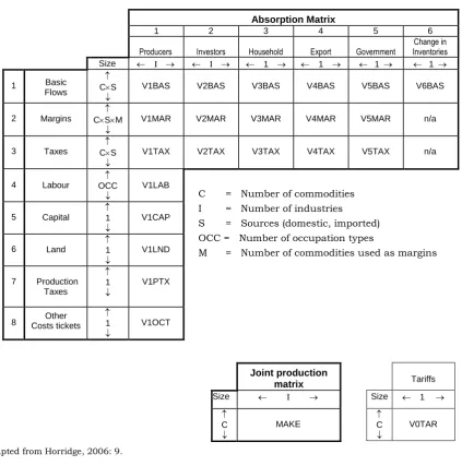
The SAGE model requires a database with separate matrices for basic, tax and margin flows for both domestic and imported sources of commodities sold to domestic and foreign users, as well as matrices for the factors of production. The structure of the IO database is illustrated in Figure 1 and the ingredients in the database are listed in Table 1. The first three rows form the absorption matrix, rows 4 to 8 the production matrix and the two satellite matrices are the multi-production matrix and the tariff matrix.

In the absorption matrix, users are identified in the column headings and denoted by a number:

1. domestic producers divided into i industries; 2. investors divided into i industries;

3. a single representative household;

4. an aggregate foreign purchaser of exports;

5. government demand; and

6. changes in inventories.

The matrices in the first row, that is, V1BAS to V6BAS, represent direct flows of commodities, from all sources to users valued at basic prices. The first matrix, V1BAS, can be interpreted as the direct flow of commodity c, from source s, used by industry i as an input into current production. V2BAS shows the direct flow of commodity c, from source s, used by industry i as an input to capital formation. V3BAS shows the flow of commodity c from source s that is consumed by a representative household. V4BAS is a column vector and shows the flow of commodity c to exports. V5BAS and V6BAS show the flow of commodity c from source s to the government and change in inventories respectively. In the IO database, no imported commodity is exported without being processed in a domestic industry. Hence, V4BAS has no import dimension.

(14)

2

the values, with the exception of V6BAS, are positive. V6BAS records the change in inventories, and thus can be positive or negative.

Figure 1. The SAGE input–output database

Absorption Matrix

1 2 3 4 5 6

Producers Investors Household Export Government Inventories Change in

Size I I 1 1 1 1 1 Basic

Flows

 CS



V1BAS V2BAS V3BAS V4BAS V5BAS V6BAS

2 Margins

 CSM



V1MAR V2MAR V3MAR V4MAR V5MAR n/a

3 Taxes

 CS



V1TAX V2TAX V3TAX V4TAX V5TAX n/a

4 Labour

 OCC



V1LAB

C = Number of commodities I = Number of industries

S = Sources (domestic, imported) OCC = Number of occupation types

M = Number of commodities used as margins 5 Capital

 1 

V1CAP

6 Land

 1 

V1LND

7 Production Taxes

 1 

V1PTX

8 _{Costs tickets}Other  1 

V1OCT

Joint production

matrix Tariffs

Size I  Size 1  C  MAKE   C  V0TAR 

The second row, V1MAR to V5MAR, represents the value of commodities used as margins to facilitate the basic flows in row 1. SAGE includes two margin commodities, trade and transport services. All margins are produced domestically. V1MAR and V2MAR are four-dimensional matrices and show the cost of margin service m used to facilitate the flow of commodity c, from source s to industry i. V3MAR and V5MAR are three dimensional and show the cost of margin service m that facilitates the flow of commodity c from source s to the representative household and the government respectively. V4MAR is a two-dimensional matrix and shows the cost of margin service m that facilitates commodities flows to exporters. There are flows that do not require any margins and therefore the values in these

(15)

3

matrices are zero or the matrices are omitted. This is mainly for services and inventories (unsold commodities) (United Nations, 1999: 33).

The third row represents the tax matrices, V1TAX to V5TAX. These matrices show the taxes paid in the delivery of domestic and imported commodities to the different users. Positive values refer to taxes and negative values to subsidies. For example, a positive element in V1TAX and V2TAX can be interpreted as the tax associated with the delivery of commodity

c from source s used by industry i as an input into current production and capital formation respectively. A negative value is interpreted as a subsidy paid on commodity c,

from source s, used by industry i. V3TAX and V5TAX are interpreted as the taxes associated with the delivery of commodity c from source s used by households and government. V4TAX is associated with the taxes paid for the delivery of commodities to exporters. Taxes are not paid on inventories and therefore there is no V6TAX matrix. It should be noted that tax rates may differ between users and sources.

Rows 4 to 6 contain matrices that provide a breakdown of the primary factors used by industry in current production. These matrices include the inputs of three factors of production: occupation-specific labour (V1LAB), fixed capital (V1CAP) and agricultural land (V1LND). For example, V1LAB shows the purchase of labour of skill o by industry i that is used as an input into current production. V1CAP contains the rental value of each industry’s fixed capital and V1LND shows the rental value of agricultural land used by each industry. Industry also pays production taxes such as business licences, payroll taxes and stamp duties (United Nations, 1999: 26). These taxes are contained in V1PTX in row 7. Other cost tickets are contained in matrix V1OCT in row 8. This is a useful device that allows for the cost of holding liquidity, cost of holding inventories and other miscellaneous production costs (Dixon et al., 1982: 70). The database shows that labour, capital, land, production costs and other cost tickets are only used in current production and therefore these matrices are absent from entries in the capital formation, household consumption, exports, government and change in inventories columns.

The satellite matrices illustrate the multi-production matrix (MAKE) and tariff matrix. Each element in the MAKE matrix refers to the basic value of commodity c produced by industry

(16)

4

produce a combination of output commodities that will maximise their revenue. For example, as the market price of commodity 1 increases relative to commodity 2, producers will shift their resources to producing more of commodity 1 and away from commodity 2.

The final matrix, V0TAR, contains tariff revenue by imported commodity. The tariff matrix is separate from the absorption matrix because the values of tariff revenues are already included in the basic price of imports, that is, they are already included in the basic flows in row 1. It enables the calculation of ad valorem rates as the ratio between tax revenues and the relevant basic flows of commodities on which the taxes are levied.

The interpretation of the columns and rows is important and should adhere to the following conditions:

 industry cost should equal industry sales (see Section 2.4.12). For all industries, the industry costs (sum across all inputs in column 1) should equal

the basic values of industry output

_{ }



 

 







, c i c COM

MAKE ;

 total domestic output should equal their total use (see Section 2.4.12). For non-margin commodities the domestic use of commodities (sum across all users in

row 1) should equal the basic value of industry output

_{ }



 

 







, c i i IND

MAKE . For

margin commodities, the use of commodity m should equal the sum of all direct usage of m (row 1 in Figure 1) plus the sum of all usage of m as a margin (row 2 in Figure 1); and

(17)

5

Table 1. Contents of the SAGE Input–Output data files

TABLO

name Name Dimension

1. Sets COM IND SRC MAR OCC

Set COM commodities Set IND industries Set SRC sources

Set MAR margin commodities Set OCC occupations

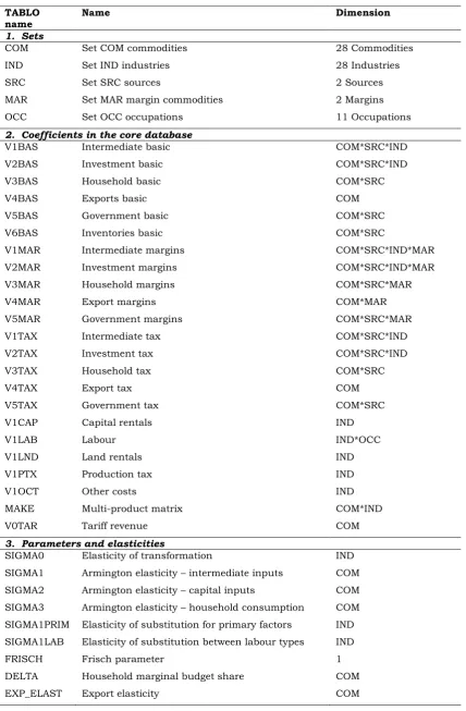
28 Commodities 28 Industries 2 Sources 2 Margins 11 Occupations 2. Coefficients in the core database

V1BAS V2BAS V3BAS V4BAS V5BAS V6BAS V1MAR V2MAR V3MAR V4MAR V5MAR V1TAX V2TAX V3TAX V4TAX V5TAX V1CAP V1LAB V1LND V1PTX V1OCT MAKE V0TAR Intermediate basic Investment basic Household basic Exports basic Government basic Inventories basic Intermediate margins Investment margins Household margins Export margins Government margins Intermediate tax Investment tax Household tax Export tax Government tax Capital rentals Labour Land rentals Production tax Other costs Multi-product matrix Tariff revenue COM*SRC*IND COM*SRC*IND COM*SRC COM COM*SRC COM*SRC COM*SRC*IND*MAR COM*SRC*IND*MAR COM*SRC*MAR COM*MAR COM*SRC*MAR COM*SRC*IND COM*SRC*IND COM*SRC COM COM*SRC IND IND*OCC IND IND IND COM*IND COM 3. Parameters and elasticities

SIGMA0 SIGMA1 SIGMA2 SIGMA3 SIGMA1PRIM SIGMA1LAB FRISCH DELTA EXP_ELAST

Elasticity of transformation

Armington elasticity – intermediate inputs Armington elasticity – capital inputs

Armington elasticity – household consumption Elasticity of substitution for primary factors Elasticity of substitution between labour types Frisch parameter

(18)

6

1.2. Parameters

In this section the parameters required by SAGE during simulations are listed. Elasticities govern the magnitude by which economic agents adjust their behaviour due to changes in for example relative price. A detailed explanation is included in Section 5.

SIGMA1PRIM denotes the constant elasticity of substitution (CES) between the three primary factors, labour, land and capital, while SIGMA1LAB denotes the CES elasticity between skills types in industry

i

. SIGMA0 represents the constant elasticity of transformation (CET) and governs the behaviour of multi-product industries that choose their output to maximise revenue. SIGMA1, SIGMA2 and SIGMA3 are the Armington elasticities and reflect the degree of substitution between domestic and imported commodities for use in current production, capital formation and household consumption.

The FRISCH parameter shows the relationship between households’ total expenditure and their luxury expenditure in the linear expenditure system (LES). DELTA denotes the household marginal budget shares. These are used to calculate the expenditure elasticities (EPS) in the household demand equations. EXP_ELAST is a vector of foreign-demand elasticities for South African commodities.

1.3. Data required for SAGE’s dynamic equations

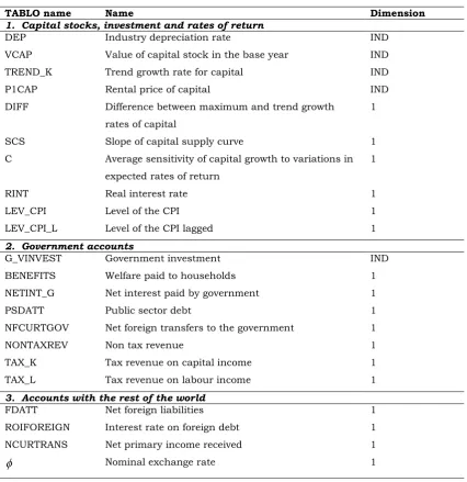
SAGE requires data for the model’s dynamic features. These data are summarised in Table 2. The first block of data lists the data and parameters required to use the rate of return and capital accumulation theory. Equations in the model require industry-specific depreciation rates, capital stock and trend growth rates for capital. Industry-specific depreciation rates are used in the capital accumulation equations as well as setting the maximum and minimum capital growth rates. DIFF is a parameter and is used to set the maximum industry capital growth rates. SCS is the reciprocal of the slope of the economy-wide capital supply curve. Kgr_i is the capital growth rate and RINT is the real interest rate.

The final two scalars relate to the inflation rate. LEV_CPI and LEV_CPI_L are calculated from the base data for the beginning and end of the base year and are used to calculate inflation. The compilation of the capital and investment data is explained in Section 2.11, Step 11.

(19)

7

(NONTAXREV). The final two data requirements are the tax rates on capital and income. The tax rates are used to calculate the direct tax revenue collected from capital and labour. The compilation of the government data is explained in Section 5.2.

Table 2. Contents of the additional data files

TABLO name Name Dimension

1. Capital stocks, investment and rates of return DEP VCAP TREND_K P1CAP DIFF SCS C RINT LEV_CPI LEV_CPI_L

Industry depreciation rate

Value of capital stock in the base year Trend growth rate for capital

Rental price of capital

Difference between maximum and trend growth rates of capital

Slope of capital supply curve

Average sensitivity of capital growth to variations in expected rates of return

Real interest rate Level of the CPI Level of the CPI lagged

IND IND IND IND 1 1 1 1 1 1 2. Government accounts

G_VINVEST BENEFITS NETINT_G PSDATT NFCURTGOV NONTAXREV TAX_K TAX_L Government investment Welfare paid to households Net interest paid by government Public sector debt

Net foreign transfers to the government Non tax revenue

Tax revenue on capital income Tax revenue on labour income

IND 1 1 1 1 1 1 1 3. Accounts with the rest of the world

FDATT ROIFOREIGN NCURTRANS



Net foreign liabilities Interest rate on foreign debt Net primary income received Nominal exchange rate

1 1 1 1

(20)

8

This concludes the description of the database requirements for the SAGE model. The remainder of this chapter describes the data sources and the steps taken to create each of the elements in the database.

2. DATA SOURCES

2.1. Note on the valuation of the tables

The 1993 System of National Accounts (SNA) recommends three ways in which production (output) of goods and services can be measured (Statistics South Africa, 2006c: 12; United Nations, 1999: 55). The definitions of these measures are given below.

Basic price: “The basic price is the amount receivable by the producer from the purchaser for a unit of a good or service produced as output, minus any tax payable (i.e. VAT and excise duties), and plus any subsidy receivable, on that unit as a consequence of its production or sale. Basic prices exclude any transport charges involved separately by the producer” (United Nations, 1999: 55).

Producers’ price: “The producers’ price is the amount receivable by the producer from the purchaser for a unit of a good or service produced as output, minus VAT, or similar deductible tax, invoiced to the producer. It excludes any transport charges invoiced separately by the producer” (United Nations, 1999: 55).

Purchasers’ price: “The purchasers’ price is the amount paid by the producer, excluding any deductible VAT or similar deductible tax, in order to take delivery of a unit of good and service at the time and place required by the purchaser. The purchasers’ price includes any transport charges paid separately by the purchaser to take delivery at the required time and place” (United Nations, 1999: 55).

2.2. Basic structure of the Supply–Use tables for South Africa (2002)

The primary source of data is the Supply–Use tables (SUTs), published in 2002 by Statistics South Africa (2006c).1_{The Supply table (ST) contains information on the supply of} commodities from all sources whereas the Use table (UT) shows the final users of these commodities.

1_{A new set of Supply-Use table for 2005 are available. A number of the data manipulating step described in this}

(21)

9

2.2.1. The Supply table (ST)

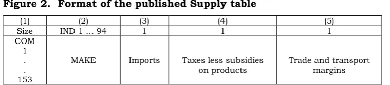
A simplified illustration of the Supply table is depicted in Figure 2. The first matrix, MAKE, shows the production of 153 domestic commodities (rows) and 94 domestic industries (columns) at basic price. The MAKE matrix is not diagonal, implying that an industry may produce more than one product and a product may be produced by more than one industry.

Figure 2. Format of the published Supply table

(1) (2) (3) (4) (5)

Size IND 1 … 94 1 1 1

COM 1

. . 153

MAKE Imports Taxes less subsidies

on products

Trade and transport margins

The next matrix (column 3), Imports, is a vector of 153 commodities supplied by imports again valued at basic price.Total supply valued at basic prices is calculated by adding the domestically produced commodities with the imported commodities.

Total supply valued at basic price is transformed into producers’ price by adding the next matrix (column 4), which contains net taxes on commodities. This is a vector of 153 commodities and consists of VAT, excise taxes, fuel levies and import duties. Subsidies on products are recorded in a similar way.

By adding column 5 (trade and transport margins), total supply at purchasers’ price is calculated. The total supply of commodities at purchases’ price is equal to the total use at purchases’ price. The total use of commodities valued at purchasers’ price is presented in the UT.

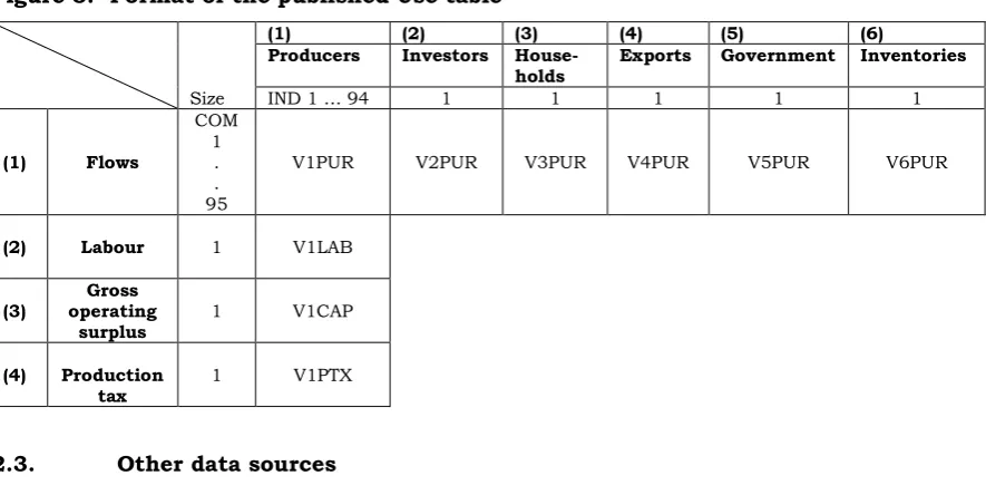
2.2.2. The Use table (UT)

(22)

10 Figure 3. Format of the published Use table

(1) (2) (3) (4) (5) (6)

Producers Investors

House-holds Exports Government Inventories

Size IND 1 … 94 1 1 1 1 1

(1) Flows

COM 1

. . 95

V1PUR V2PUR V3PUR V4PUR V5PUR V6PUR

(2) Labour 1 V1LAB

(3) operating Gross

surplus 1 V1CAP

(4) Production

tax

1 V1PTX

2.3. Other data sources

As well as the SUT, various other sources of data were used for verification, aggregation or disaggregation of data, or for borrowing shares to facilitate the creation of related matrices.

2.3.1. Social accounting matrix (2002)

In addition to the SUT, Statistics South Africa published the Social Accounting Matrix (SAM) for 2002. The SAM integrates the SUT and institutional-sector accounts into a single matrix format. The main focus of the 2002 SAM is on households and their income and expenditure patterns. The population is divided into four population groups and 12 household expenditure groups. Several additional labour matrices are introduced. These labour matrices provide additional information regarding the labour distribution across industry and occupation by persons and wage bills. It should be noted that the dimensions in the SUT and SAM are different. The SUT dimensions are mapped to the SAM dimensions. This is explained in Section 2.4.1, Step 1.

2.3.2. South Africa Reserve Bank Quarterly Bulletin

The South African Reserve Bank (SARB) publishes the Quarterly Bulletin (SAQB) which contains the National Accounts. These accounts were used to compare the values organised in the SUT with those published in the SAQB. Comparisons were made for value added by industry, capital formation, exports, imports, taxes and margins. The Quarterly Bulletin was also helpful in creating the government accounts. The data in the December (2005)

(23)

11

2.3.3. Government accounts

It was very difficult to find consistent government data. Treasury, Statistics South Africa and the Reserve Bank publish government data, but the data are not consistent, which makes comparison very difficult. The December 2005 Quarterly Bulletin contains information on government accounts which is broadly consistent with the government information in the SUT. The information in the SAQB is used to create the government accounts.

2.3.4. Use of GTAP data to specify land rents

The GTAP 6.0 database (Dimaranan, 2006) includes an extra factor of production, namely land. None of the above data sources explicitly provides data on land and therefore the GTAP database for South Africa is used to create land rentals for the agricultural and mining industries.

2.3.5. Sector-specific data

In the SUT and SAM, gross fixed capital-formation data is given as a vector. This vector shows which commodities are used for investment by a single aggregate investor. However, SAGE requires capital formation to be disaggregated by industry. Hence, industry-specific information is required so that the single investment column can be split into 28 industry columns. The Annual Financial Statistics Survey is used to obtain such industry-specific data (Statistics South Africa, 2006a).

3. STAGES IN THE CONSTRUCTION OF THE SAGE DATABASE

The core database required by SAGE is described in Section 1 and Figure 1. The final SAGE database, which fits this form, includes 28 commodities, 28 industries, 11 occupational groups, two margin commodities and two sources. The elements of the different dimensions (sets) are listed in Appendix 1. Although the SUT conforms to the international statistical standards for the measurement of an economy as set out in the 1993 System of National Accounts (SNA), it is not in the correct format needed for the SAGE database. Several steps were taken to convert the published data into the required format. These steps are discussed in this section.

(24)

12

manipulation process addresses a specific data query and the output of a step is used as an input in the next step. The process is as follows (Horridge, 2006):

 Data are converted from their original hard copy or Excel format into Header Array files;

 Each data manipulation process is programmed in a TABLO file. The TABLO file includes all the data manipulation equations, written in TABLO code, and uses the VIEWHAR files as input files; and

 To make sure that the balancing requirements are not violated test or check

commands are included in each step.

This automated process has a number of advantages. Firstly, each TABLO file serves as a record of the process used to manipulate the data. Secondly, adjustments and corrections to formulas can easily be made. Thirdly, the automation enables fast replications of the process when needed. This is very useful when new data becomes available. Finally, recording each step promotes transparency and avoids any “black box” issues, that is, the data programs become a permanent documentation of the data manipulation process. The next section describes the steps taken to convert the published data into the required IO database.

3.1. Step 1: Data mapping and aggregation

The dimensions of the SAGE database differ from those of the published data. SAGE includes an aggregated database with the dimensions of 28 commodities, 28 industries, 11 occupational groups, two margin commodities and two sources. There are several reasons to support a smaller, aggregated database. Firstly, the aggregated database ensures improved management of data. Secondly, most of the secondary data used to verify or compare data, are published either on a macro level or on a highly aggregated level. Thirdly, when it is necessary to disaggregate a commodity or industry, it is easier to adapt shares from other sources. Finally, it is not necessary to include a highly disaggregated database. The focus of this thesis is on the effects of HIV/AIDS on the labour market with specific emphasis on labour supply. The emphasis is to ensure that (1) the linkages between SAGE and the health extension are correct and (2) that the dynamic features are operational. If required, the core database can be disaggregated.

The commodities and industries, as they appear in the SUT, are mapped to 272_commodities and industries by using the Standard Industrial Classification of all Economic Activities (SIC) (Statistics South Africa). The GEMPACK program, VIEWHAR, was used to turn

2_{The final database includes 28 commodities and 28 industries. The additional commodity and industry (Owner}

(25)

13

spreadsheet data into entries in a single HAR file called FID.HAR. An additional file,

SETINFO, is also created where all the set information is organised. This file remains the same in all steps.

Firstly, the 153 commodities are mapped to 27 commodities and the 94 industries are mapped to 27 industries (Statistics South Africa, 2006c: 46). The mapping of commodities and industries is useful in identifying any misprints and irregularities that may be present in the data. Since, in this step, no data adjustment has occurred and in the absence of any irregularities, the mapped data should correspond to the published SAM data. No misprints or irregularities were noted.

3.2. Step 2: Distribution of the residual

The output files of Step 1, FID.HAR and SETINFO.HAR, are used as input files in Step 2. The Use tables include a commodity-specific residual. This residual is included because GDP calculated according to the production and income approach, differs from GDP calculated from the expenditure side. Firstly, the production and generation of income accounts are compiled for each industry. These accounts are consistent with both the production and income approach. GDP is therefore calculated from the supply side and then transferred to the demand side (Use table). Secondly, the values for the components of final demand, as they appear in the Use table, are then adjusted to be consistent with the values published by the South African Reserve Bank (SARB). The SARB calculates GDP using the expenditure approach. Their estimations allow for the compilation of the goods and services account in which the residual item can be calculated.

In the 2002 SUT the residual item is negligible and therefore allocated to the “change in inventories” vector. This ensures that commodity-specific aggregated supply is equal to commodity-specific aggregate demand with only the “change to inventory” vector changed.

3.3. Step 3: Adjustments to the Supply and Use table

(26)

14

To preserve the condition that commodity-specific aggregate supply should equal commodity-specific aggregate demand, the same commodity shares are used when the “purchases by residents abroad” is distributed. I use the commodity-specific household expenditure shares3_{, which are multiplied by 19,601 to determine the commodity-specific} purchases by residents abroad. These values are then added to the original commodity-specific household expenditure and commodity-commodity-specific imports (United Nations, 1999: 154). This is the first step illustrated in Figure 4.

“Purchases by non-residents” (R20,732 million) in South Africa are included in the household expenditure column. As this represents expenditure by foreigners, it should be deducted from domestic household expenditure and treated as exports (United Nations, 1999:33). To keep the SUT balanced, the same household expenditure shares, which are used to distribute the “purchases by residents abroad”, are used to adjust commodity-specific household expenditure and exports with the “purchases by non-residents”. Purchases by non-residents are added to exports and deducted from household expenditure. This is Step 2 in Figure 4.

Figure 4. Adjustment of purchases by residents abroad and non-residents domestically

3_{The commodity-specific household expenditure shares are calculated as}

      _  



c c c c COM HHEXP HH SHR HHEXP , with

commodities referring to all the commodities that households consume.

c = commodity

HH_SHR (c) H’hold expenditure share Purchases by residents abroad (c) add add (2) (3) minus minus (2) (1) (2) multiply multiply (1) Purchases by non-residents in South Africa Purchases by residents abroad V3PUR(c) Household expenditure IMPS(c) Imports CIF/FOB adjustment(c) Purchases by non-residents in South Africa (c)

(27)

15

The final adjustment is regarding imports and is shown in Step 3 in Figure 4. The imports of goods CIF includes the value of imported goods FOB and transport and insurance services rendered by both residents and non-residents. However, when the latter services are rendered by non-residents, they are already included in the imports of services. Similarly, when these services are rendered by residents they are considered to be domestic output and cannot be included in the imports column. If no adjustment is made, imports will be overestimated by the value of transport and insurance services rendered by both residents and non-residents. To adjust imports, adjustments are introduced to correct the two relevant service commodities. The adjustment value is the total value of transport services (R18,639 million) and insurance services (R2,093 million) rendered by both residents and non-resident producers. These values are deducted from the import value for that specific commodity (United Nations, 1999: 31).

3.4. Step 4: Check that aggregate supply is equal to aggregate demand

To ensure that the adjustments in the previous steps were correctly implemented, this step is introduced to confirm that the Input–Output table is still balanced, that is, aggregate demand is equal to aggregate supply when valued at the same price.

Commodity-specific supply valued at purchases’ price is given as:

 c  c i,  c  c  c

i IND

SUPPLY MAKE IMPORT MARGINS TAX 





   (E4.1)

where  MAKE

_{ }

_c is the domestic production of commodity c, summed across all

domestic industries i;

 IMPORT_{ }_c is the commodity-specific imports after the CIF/FOB adjustment;

 MARGINS

_{ }

_c refers to the margins associated with each commodity c; and

 TAX

_{ }

_c refers to commodity taxes less subsidies for each commodity c.

Commodity-specific demand valued at purchases’ prices is given as:

 

1

 

2

 

3

 

4

 

5

 

6

 

 









   

c c i c i c c c c

i IND i IND

DEMAND V PUR _, V PUR _, V PUR V PUR V PUR V PUR

(E4.2)

where  V PUR1

_{ }

_{c i}_, and V PUR2

_{ }

_{c i}_, are the commodity and industry-specific flow

(28)

16

production) and user 2 (investors). These flows are summed across industries;

 V PUR3

_{ }

_c is the commodity-specific flow values, after all adjustments have

been made for user 3 (households);

 V PUR4

_{ }

_c is commodity-specific flow values for user 4 (exports);

 V PUR5

_{ }

_c is commodity-specific flow values for user 5 (government); and

 V PUR6

_{ }

_c is commodity-specific flow values for user 6 (inventories).

This check confirms that the adjustment had been performed correctly.

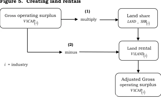
3.5. Step 5: Creating land rentals

SAGE distinguishes between three types of factors of production: labour, capital and land. The UT includes information on compensation of employees (COE), gross operating surplus (GOS) and production taxes. There are no values for land rentals. I therefore allocate some part of the gross operating surplus to land-using4_{industries. The share of land, as it} appears in the GTAP 6.0 database for South Africa, is used to determine the share of gross operating surplus allocated to land rentals (Dimaranan, 2006).

The industries that use land in the production process are agriculture, coal, gold, and other mining. The percentage of gross operating surplus that is allocated to land rentals, that is, the land share, is 15 per cent for agriculture and 30 per cent each for the remaining land-using industries. For non-land-land-using industries, none of the gross operating surplus was allocated to land.

Figure 5. Creating land rentals

4_{Land refers to cultivated land area, forests and natural resources such as minerals, gold and oil.}

i = industry

Land share

 i

LAND_SHR

multiply

Adjusted Gross

operating surplus

 

1 _i

V CAP

Gross operating surplus

 

1 _i

V CAP

minus

(1)

(2)

Land rental

 

1 _i

(29)

17

3.6. Step 6: Splitting total flows into sources

SAGE requires the VBAS, VMAR and VTAX flow matrices, the first three rows in Figure 4.1, to be split into domestic and imported flows. The task at hand is to distribute imports across users. However, this task is made difficult because I only know the commodity-specific import value. Since there is no information available on user-commodity-specific imports, I assume that the share of imports in total use of commodity c, is the same for all users. For example, if imported meat makes up 10 per cent of total sales (use) of meat from both domestic and imported sources, then all users of meat will use 10 per cent of imported meat in their meat purchases.

The commodity-specific flows, as they appear in the Use table, are valued at purchasers’ prices and include imports. Because it is assumed that (1) no imported commodity is re-exported and (2) the percentage of imports used by each user is the same as the share of imports in total use, the import share5_{of each commodity can be calculated. To determine} how much of each commodity is imported, this share is then multiplied by each user’s total use of a commodity. This is illustrated by the first step in Figure 6. The user-specific domestic flows are calculated by deducting the user-specific imported flow from the total use of that commodity. This is illustrated by Step 2 in Figure 6. Step 3 in Figure 6 illustrates the user-specific matrices including the source dimension.

Figure 6. Creating source dimensions: domestic and imports

5

 

0 ,

_ _c c c

c u u USERS

IMPORTS V TARf

IMP SHR

VPUR

  



where u refers to the following users, (1) current production, (2) investors,

(3) private consumption, (4) exports (5) public consumption and (6) change in inventories. Because no imported good is re-exported, there is no import dimension for any of the flows associated with exports.

(1) _minus

u = users

c = commodities

s = source (domestic or import)

i = industry

(1) (2)

(3)

Total user-specific flows at purchasers’

price VPUR_ S

_{ }

_{c u}_,

Import user share

 

IMP_ SHR_c

User-specific flows at purchasers’ price

including source



c s u



VPUR _{, ,}

multiply

Commodity-specific imports for every user



c IMP u



VPUR _, _,

Domestically produced commodities for every

user



c DOM u



VPUR _, _,

(30)

18

3.7. Step 7: Creating an “Ownership of Dwellings” commodity and industry

In the original SUT there was no explicit recognition of the imputed value of owner-occupied dwellings (OwnerDwel). Ownership of dwellings is an important component of household expenditure as it is closely linked to household income and as such can give additional insight into the economic wellbeing of the population. In a dynamic setting, we would also expect that as per capita income increases, the household budget share of dwellings will also increase. It is therefore important, for proper modelling of civil construction and non-dwelling consumption of commodities, to explicitly model household demand for non-dwellings.

According to the latest Income and Expenditure Survey (IES), 23.6 per cent6_{of total} household consumption is spent on housing, water, electricity, gas and other fuels (Statistics South Africa, 2008b). Housing includes the:

 annual rental value of a dwelling unit; or

 the annual estimated rental value of the dwelling unit if the unit was rented free in the case of rented dwelling units; or

 if it is an owner-occupied dwelling unit, 7 per cent of the value of the dwelling unit (Statistics South Africa, 2008b and United Nations, 1999: 134).

In this section the creation of the Owner Dwellings sector, with an appropriate cost and sale structure, is explained. In the SUTs, Owner Dwellings is originally included in the Real Estate7_{sector. This sector is disaggregated into a}_{Real Estate}_{sector, which mainly captures} fee-paying real estate activities, and an Owner Dwelling sector, which represents the housing stock.

There are two specific characteristics that distinguish the Owner Dwellings commodity from other commodities. Firstly, Owner Dwellings are only produced domestically. No Owner Dwellings are imported, and secondly, the commodity Owner Dwellings is only consumed by households. The industry, Owner Dwellings, only uses intermediate commodities and capital as a primary input in the construction of dwellings. No land or labour is used.

To disaggregate the Total Real Estate sector, the following information regarding Owner Dwellings is needed (1) the value of outputs, (2) input structure, and (3) sales structure.

6_{The 23.6 per cent includes: Actual rentals for housing (3.6%), Imputed rentals for housing (12.6%), Maintenance}

and repair of the dwelling (1.7%), Water supply and miscellaneous services relating to the dwelling (3.2%) and Electricity, gas and other fuels (2.4%) (Statistics South Africa, 2008: 46).

7_{Real Estate falls under major division 8 in the SIC, and consists of Real Estate Activities with own or leased}

(31)

19

3.7.1. Value of output

The National Accounts for 2002 shows the value of rents8_{as R65,633 million (SARB, 2005:} S–118). In the SUT, the value for Real Estate, which includes Owner Dwellings, is R62,508 million. This discrepancy may be due to the purchases by residents abroad and purchases by non-residents domestically.

Based on information in the IES and National Accounts data, I assumed that housing comprises approximately 8 per cent of total household expenditure as it appears in the SUT. This percentage is slightly higher than the 7.2 per cent share of Dwellings in the world’s private household consumption in the GTAP 6.0 database. The calculated value of output of the Owner Dwellings sector is R57,762 million, which is approximately 93 per cent of the total value of Real Estate in household expenditure. This share is used to split the Total Real Estate element into two separate elements called Owner Dwellings and Real Estate.

3.7.2. Sales structure

It is assumed that households are the only users who consume the commodity Owner Dwellings. Hence, the sales structure of Owner Dwellings is known. The sales structure of a commodity is indicated by row 1 in Figure 1. Households spend R57,767 million on the commodity, Owner Dwellings. This value is then subtracted from Total Real Estate to determine the Real Estate commodity dealing mostly with real estate services. This implies that:

3 ( ," ") ,57 762

V BAS OwnerDwel dom R million and

3 (Real ," ") = 3 ( Real ," ") 3 ( ," ")

V BAS Estate dom V BAS Total Estate dom V BAS OwnerDwel dom

(E4.3)

No other user buys the commodity Owner Dwellings, and therefore the corresponding flows from this commodity to those users are set to zero. For all other users the Real Estate value remains the same.

3.7.3. Input structure

The next step is to split the Total Real Estate column into an Owner Dwellings column and

Real Estate column. This is difficult because of (1) lack of information regarding industry-specific input and cost structures and (2) the input structure of the industries may differ.

(32)

20

Due to the lack of information, the cost structure for the Owner Dwellings industry is based on MONASH data. Hence, for each of the Owner Dwellings and Real Estate industries (1) the source-specific intermediate input commodities and (2) the share in which each of these commodities are used are borrowed from the MONASH database. The shares of the source-specific intermediate commodities used by the Owner Dwellings industry are listed in Appendix 4E.

The next step is to determine, for both the Real Estate and Owner Dwellings industry, what percentage of the cost structure will be allocated to source specific intermediate inputs and primary inputs. It is assumed that the Owner Dwellings industry only uses capital in the production process. For the cost shares pertaining to Owner Dwellings, I base my decision on the MONASH cost shares. In the MONASH database, 17 per cent of total cost are

allocated to domestic commodities used as intermediate

inputs



V BAS c dom1



," ","OwnerDwel"



, 1 per cent is allocated to imported commodities used

as intermediate inputs



V BAS c imp1



," ","OwnerDwel"



and 82 per cent are allocated to capital







V CAP1 "OwnerDwel"



. The cost structure9 of the Real Estate industry is the difference

between the values of the original Real Estate industry and Owner Dwellings, that is:

1 ,"Real Estate"  1 Real Estate"  1 ,"OwnerDwel"

V BAS c s(, ) V BAS c s(, ," ) (,V BAS c s ) (E4.4)

No other commodity is used by the Owner Dwellings industry as an input in current production and therefore all the remaining elements are set to zero. The elements of the commodity and industry sets have increased from 27 to 28.

After this split, the database is slightly unbalanced. This imbalance is corrected in Step 12.

3.8. Step 8: Creating margin matrices

The output of wholesalers and retailers is measured by the value of the trade margins realised on the goods they sell, that is, the difference between the sale value of products sold and the cost of purchasing these products. The reason for this is that the productive activity associated with distribution is understood to be the provision of services of displaying the goods in an informative and attractive way (Statistics South Africa, 2006c: 14).

Trade and transport margins are the difference between the purchasers’ price and the producers’ price of a product. It is therefore possible that a product can be sold at different

9_{The output value of the Owner Dwellings is R57,762 million. Seventeen per cent, R9,820, which is allocated to the}

(33)

21

purchasers’ prices due to differences in margins and net taxes (United Nations, 1999: 56). A clear distinction should be made between transport services and margins. Transport services move people, while transport margins move goods. Transport margins can be treated in two different ways. Firstly, when transport is arranged in such a way that the purchaser has to pay separately for the transport costs, that is, the transport costs are billed separately, it is identified as transport margins. The customer not only buys the goods, but also the transport services from producers. Secondly, if transport services are not billed separately, that is, the producer transports the goods without extra cost to the purchaser, transportation will appear as intermediate consumption to the producer and at the same time will be included in the basic price (Statistics South Africa, 2006c: 14; United Nations, 1999: 133).

For all agricultural, mining and manufacturing commodities, margins are given as the sum of trade and transport margins. The following should be noted:

 there are no margins for services provided because services are delivered directly from producers to consumers, and hence do not require margins;

 there are no margins on inventories because they comprise unfinished commodities and materials; and

 only domestically produced margins are used, i.e. margins are not imported.

Included in the margin column are two negative values. Values are negative for Trade and Transport services. The reason for this is that in the Use table, the values for trade and transport services (commodities 85 and 87) show only those that are consumed directly and do not include any margins. Instead, margins are included in the value of the goods at purchasers’ prices shown in the rest of the Use table. Consequently, in the Supply table, trade and transport margins should be deducted from the total supply of market services. This is done by entering trade and transport margins as a negative number in order to balance the supply and use of trade and transport services at purchasers’ prices (United Nations, 1999: 33).

(34)

22

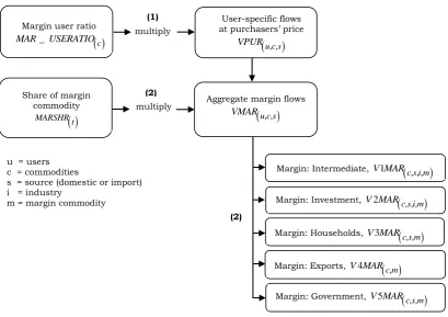
3.8.1. Calculation of aggregate margin matrices by user

In this step the margin matrices, V1MAR_M to V5MAR_M, are determined. This is done by calculating the margin-use ratio for each commodity. To create these matrices I assumed that the margin-use ratio is the same for all users, that is, if the margin-use ratio for commodity c is 8 per cent, it is 8 per cent for all users of commodity c. Secondly, the margin rate is the same for both domestic and imported commodities. Since the flows in the Use table are at purchasers’ prices, that is, include margin commodities, and given that the commodity-specific margins are given in the Supply table, the margin-use ratio is calculated.10_{The margin-use ratio is then multiplied with the user-specific flow valued at} purchasers’ prices to create the user-specific aggregate margins. This is illustrated by (1) in Figure 7.

Figure 7. Creating source dimensions for the margin matrices

3.8.2. Creating margin matrices by type of margin commodity

The next step is to distribute the aggregate user-specific margin for each commodity

10

 





 



 

c

u c s u USER s SRC

MARGIN

MAR USERATIO

VPUR _{, ,}

_ where u refers to the following users, (1) current production, (2)

investors, (3) private consumption, (4) exporters and (5) public consumption. Because inventories are unsold

commodities, there is no margin matrix associated with inventories.

(2)

u = users c = commodities

s = source (domestic or import) i = industry

m = margin commodity

User-specific flows at purchasers’ price



u c s, ,



VPUR

Margin user ratio

 

c

MAR_ USERATIO multiply

(1)

Aggregate margin flows



u c s



VMAR _{, ,}

Share of margin commodity

 

MARSHR_t

Margin: Intermediate, V MAR1

_

_{c s i m}_{, , ,}

_

Margin: Households, V MAR3

_

_{c s m}_{, ,}

_

Margin: Exports, V MAR4

_{ }

_{c m}_,

Margin: Government, V MAR5

_

_{c s m}_{, ,}

_

Margin: Investment, V MAR2

_

_{c s i m}_{, , ,}

_

(2)

(35)

23

between transport and trade margins. Since the total value of trade and transport margins is known, the share of trade and transport in total margin is calculated.11_{Again, it is} assumed that the all users use the same proportion of trade and transport margins. The margin commodity share is then multiplied with the aggregate user-specific margin. This yields margin matrices by commodity, source and user for all margin commodities. This is illustrated by (2) in Figure 7.

3.9. Step 9: Creating tax matrices

3.9.1. Defining the different taxes

Indirect taxes includes taxes on products that are payable by the user and taxes on production that are paid by producers. The SUT contains information on both these types of taxes. Commodity-specific taxes, payable by users, are recorded in the Supply table while industry-specific production taxes, payable by producers, are recorded in the Use table.

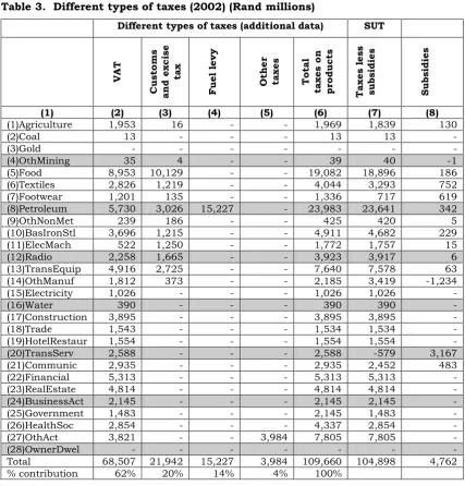
Taxes on products are payable on goods and services when they are produced, delivered, sold, transferred or otherwise disposed of by their producers and are proportional to their production values (United Nations, 1999: 26). There is only one column in the Supply table that reports commodity-specific taxes on products. SAGE requires the creation of user-specific tax matrices, V1TAX to V5TAX, which implies that the values in the tax column have to be distributed across users. This proves to be difficult because we do not know who is responsible for the tax. Additional data breaks this column into four different types of commodity taxes: VAT, customs and excise taxes, fuel levies and other taxes (Statistics South Africa, 2007). Table 3 lists these taxes and subsidies paid on each commodity. The row totals of the net taxes (column 7) are consistent with the data in the SUT. The elements in columns 2 to 5 are based on expert knowledge and the column total in column 6 is consistent with data published by the SARB (South African Reserve Bank, 2005: S-136).

VAT is by far the most important indirect tax source and contributes 62 per cent to net taxes on products. VAT is a consumption-type tax and the revenue is raised for the government by certain traders. These trades are registered and charge VAT on taxable supplies for goods and services on behalf of the government. The tax burden of the tax falls on the final consumer.

11

 

2

1 





t t

MARGIN MARSHR

MARGINS

(36)

24

Excise duties contribute 12 per cent to net taxes on products and can be levied on both domestic and imported goods.12_{Excise duties are levied on alcoholic beverages, tobacco} products and petroleum. They are also sometimes imposed to reduce consumption of certain goods (Black et al., 2007: 201).

Table 3. Different types of taxes (2002) (Rand millions)

Different types of taxes (additional data) SUT

VAT C u st o ms a nd e x c ise tax Fu e l le vy Ot he r ta xe s T o ta l ta xe s o n pr o du c ts T a xe s le ss su bsidie s S u bsidie s