5-11-2012 12:00 AM
Software Size and Effort Estimation from Use Case Diagrams
Software Size and Effort Estimation from Use Case Diagrams
Using Regression and Soft Computing Models
Using Regression and Soft Computing Models
Ali Bou Nassif
The University of Western Ontario Supervisor
Dr. Luiz Fernando Capretz
The University of Western Ontario
Graduate Program in Electrical and Computer Engineering
A thesis submitted in partial fulfillment of the requirements for the degree in Doctor of Philosophy
© Ali Bou Nassif 2012
Follow this and additional works at: https://ir.lib.uwo.ca/etd
Part of the Other Electrical and Computer Engineering Commons
Recommended Citation Recommended Citation
Bou Nassif, Ali, "Software Size and Effort Estimation from Use Case Diagrams Using Regression and Soft Computing Models" (2012). Electronic Thesis and Dissertation Repository. 547.
https://ir.lib.uwo.ca/etd/547
This Dissertation/Thesis is brought to you for free and open access by Scholarship@Western. It has been accepted for inclusion in Electronic Thesis and Dissertation Repository by an authorized administrator of
i
(Thesis Format: Integrated Article)
by
Ali Bou Nassif
Graduate Program in Electrical and Computer Engineering
A thesis submitted in partial fulfillment
of the requirements for the degree of
Doctor of Philosophy
The School of Graduate and Postdoctoral Studies
Western University
London, Ontario, Canada
ii Supervisor
______________________________ Dr. Luiz Fernando Capretz
Co-Supervisor
______________________________ Mr. Danny Ho
Supervisory Committee
______________________________
Examiners
______________________________ Dr. Abdallah Shami
______________________________ Dr. Abdelkader Ouda
______________________________ Dr. Nazim Madhavji
______________________________ Dr. Khalil El-Khatib
The thesis by
Ali Bou Nassif
entitled:
Software Size and Effort Estimation from Use Case Diagrams Using
Regression and Soft Computing Models
is accepted in partial fulfillment of the requirements for the degree of
Doctor of Philosophy
Date: May 11, 2012 _______________________________
iii
case diagrams. The main advantage of our model is that it can be used in the early stages
of the software life cycle, and that can help project managers efficiently conduct cost
estimation early, thus avoiding project overestimation and late delivery among other
benefits. Software size, productivity, complexity and requirements stability are the inputs
of the model. The model is composed of six independent sub-models which include
non-linear regression, non-linear regression with a logarithmic transformation, Radial Basis
Function Neural Network (RBFNN), Multilayer Perceptron Neural Network (MLP),
General Regression Neural Network (GRNN) and a Treeboost model. Several
experiments were conducted to train and test the model based on the size of the training
and testing data points. The neural network models were evaluated against regression
models as well as two other models that conduct software estimation from use case
diagrams. Results show that our model outperforms other relevant models based on five
evaluation criteria. While the performance of each of the six sub-models varies based on
the size of the project dataset used for evaluation, it was concluded that the non-linear
regression model outperforms the linear regression model. As well, the GRNN model
exceeds other neural network models. Furthermore, experiments demonstrated that the
Treeboost model can be efficiently used to predict software effort.
Keywords: Software Size and Effort Estimation, Use Case Diagrams, Regression
iv
encouragement, guidance and support through my entire Ph.D. program. Their
constructive feedback motivated me to conduct my research efficiently and challenged
me to publish my work in reputable conferences and journals.
I would also like to thank my wife Adeeba for her patience, support and tireless
v
Acknowledgements ... iv
Table of Contents ...v
List of Tables ... ix
List of Figures ... xii
Glossary of Terms ... xix
Chapter 1 ...1
1. Introduction ...1
1.1 Motivation ...1
1.2 Research Questions ...9
1.3 Research Contributions ... 13
1.4 Thesis Structure ... 15
References ...16
Chapter 2 ...19
2. Background ...19
2.1 Fuzzy Logic ... 19
2.2 Neural Network ... 20
2.2.1 Multilayer Perceptron (MLP) ... 22
2.2.2 Radial Basis Function Neural Network ... 23
2.2.3 General Regression Neural Network ... 25
2.3 Evaluation Criteria ... 26
2.4 Literature Review ... 29
2.4.1 Algorithmic Models ... 31
2.4.1.1 COCOMO ... 31
2.4.1.2 SLIM ... 33
2.4.1.3 Function Point Model ... 35
2.4.1.4 Use Case Point Model ... 36
vi
Chapter 3 ...60
3. MLP and Linear Regression Models ...60
3.1 Introduction... 60
3.2 Research Methodology and Models’ Evaluation ... 61
3.2.1 Regression Model ... 61
3.2.2 Fuzzy Logic Approach ... 74
3.2.3 Neural Network Model ... 77
3.3 Models Assessment and Discussion... 83
3.3.1 Testing the Proposed Models ... 83
3.3.2 Comparison Among Different Models ... 87
3.3.3 Discussion ... 88
3.4 Threats to Validity ... 88
3.5 Conclusion ... 90
References ...92
Chapter 4 ...94
4. Regression, RBFNN and GRNN ...94
4.1 Introduction... 94
4.2 Model’s Input Factors and Effort-Size Relationship ... 95
4.2.1 Size Estimation ... 96
4.2.2 Project Complexity ... 98
4.2.3 Productivity ... 100
4.2.3.1 Calibration of Productivity Factor ... 103
4.2.4 Requirements Stability ... 106
4.2.5 Effort-Size Relationship ... 108
4.3 Non-linear Regression Model ... 109
4.4 Linear Regression Model with a Logarithmic Transformation ... 118
4.5 Radial Basis Function Neural Network ... 126
vii
4.8 Models verification ... 135
4.8.1 Non-Linear Model Verification ... 136
4.8.2 Linear Model Verification ... 137
4.8.3 Neural Network models verification ... 138
4.9 Models Evaluation and Comparison ... 140
4.9.1 Project Dataset ... 140
4.9.2 Models Evaluation... 141
4.9.3 Comparison Between Models ... 151
4.9.3.1 Comparison With All Data Points ... 151
4.9.3.2 Comparison With Small Data Points ... 152
4.9.3.3 Comparison With Medium-Sized Data Points ... 152
4.9.3.4 Comparison With Large Data Points ... 153
4.10 Threats to Validity ... 154
4.11 Conclusions... 155
References ...158
Chapter 5 ...161
5. A Treeboost Model for Software Effort Estimation ...161
5.1 Introduction... 161
5.2 Decision Tree Model ... 162
5.3 Model’s Inputs ... 164
5.4 The Treeboost Model ... 166
5.5 Multiple Linear Regression Model ... 172
5.6 Model Evaluation ... 173
5.7 Discussion ... 176
5.8 Threats To Validity ... 176
5.9 Conclusions... 178
References ...180
viii
Appendix B ...192
Appendix C ...195
Appendix D ...197
Appendix E ...201
Appendix F ...203
Appendix G ...207
Appendix H ...208
ix
Table 1-2 Use case description... 8
Table 2-1 Software project types [12] ... 33
Table 2-2 Use case scenario (description)... 38
Table 2-3 Complexity weights of use cases [20] ... 38
Table 2-4 Complexity weights of actors [20]... 38
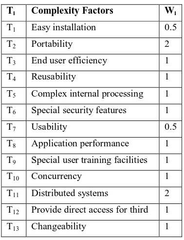
Table 2-5 Technical factors ... 41
Table 2-6 Environmental factors ... 41
Table 3-1 ANOVA for Equation 3.5 ... 72
Table 3-2 Model parameters for Equation 3.5 ... 72
Table 3-3 ANOVA for Equation 3.8 ... 72
Table 3-4 Model parameters for Equation 3.8 ... 72
Table 3-5 Productivity factor ... 75
x
Table 3-9 Results using small projects ... 85
Table 3-10 Results using large projects ... 86
Table 4-1 Use case complexity ... 98
Table 4-2 Productivity factor ... 103
Table 4-3 New productivity factor ... 106
Table 4-4 Non-linear equations ... 111
Table 4-5 Linear model parameters ... 119
Table 4-6 RBFNN parameters... 130
Table 4-7 GRNN spread value ... 132
Table 4-8 Non-linear regression verification ... 137
Table 4-9 Linear regression verification ... 138
Table 4-10 Neural network models verification ... 139
xi
Table 4-14 Models evaluation- large range... 144
Table 5-1 Model's Parameters ... 170
Table 5-2 Evaluation results ... 174
xii
Figure 1-2 Use case diagram [6] ... 5
Figure 2-1 Activation functions [3] ... 21
Figure 2-2 Schematic diagram of a MLP model ... 23
Figure 2-3 Schematic diagram of a RBFNN model [5] ... 24
Figure 2-4 Schematic diagram of a GRNN model [7] ... 25
Figure 2-5 Putnam’s time-effort graph based on Rayleigh distribution [13] ... 34
Figure 2-6 High level view of the function point model ... 36
Figure 3-1 Histogram of size ... 64
Figure 3-2 Histogram of effort ... 64
Figure 3-3 Histogram of ln(Size) ... 65
Figure 3-4 Histogram of ln(Effort)... 65
Figure 3-5 Comparison between software size and software effort ... 67
xiii
Figure 3-9 Mamdani output membership Function ... 75
Figure 3-10 Neural network model ... 79
Figure 3-11 Performance graph... 82
Figure 3-12 Regression graph ... 82
Figure 3-13 MMER interval plot ... 85
Figure 3-14 MMER interval plot for small projects ... 86
Figure 3-15 MMER interval plot for large projects ... 87
Figure 4-1 Mamdani input membership function ... 104
Figure 4-2 Mamdani output membership function ... 104
Figure 4-3 Requirements stability ... 107
Figure 4-4 Comparison between UCP model and actual data ... 109
Figure 4-5 Polynomial, all data ... 112
xiv
Figure 4-9 Polynomial, small data ... 114
Figure 4-10 Exponential 1, small data ... 114
Figure 4-11 Exponential 2, small data ... 114
Figure 4-12 Exponential 3, small data ... 115
Figure 4-13 Polynomial, medium data ... 115
Figure 4-14 Exponential 1, medium data ... 115
Figure 4-15 Exponential 2, medium data ... 116
Figure 4-16 Exponential 3, medium data ... 116
Figure 4-17 Polynomial, large data ... 116
Figure 4-18 Exponential 1, large data ... 117
Figure 4-19 Exponential 2, large data ... 117
Figure 4-20 Exponential 3, large data ... 118
xv
Figure 4-24 Effort, small data ... 121
Figure 4-25 Size, medium data ... 121
Figure 4-26 Effort, medium data ... 121
Figure 4-27 Size, large data... 122
Figure 4-28 Effort, large data ... 122
Figure 4-29 ln (Size_All_Data) ... 122
Figure 4-30 ln (Effort_All_Data) ... 122
Figure 4-31 ln (Size_Small_Data)... 122
Figure 4-32 ln (Effort_Small_Data) ... 122
Figure 4-33 ln (Size_Medium_Data) ... 123
Figure 4-34 ln (Effort_Medium_Data) ... 123
Figure 4-35 ln (Size_Large_Data)... 123
xvi
Figure 4-39 ln(size/effort), medium data ... 124
Figure 4-40 ln(size/effort), large data ... 125
Figure 4-41 Size/effort, all data... 125
Figure 4-42 Size/effort, small data ... 125
Figure 4-43 Size/effort, medium data ... 126
Figure 4-44 Size/effort, large data... 126
Figure 4-45 Size/ effort relationship ... 128
Figure 4-46 Number of neurons ... 129
Figure 4-47 Actual versus predicted effort ... 130
Figure 4-48 Actual versus predicted target (GRNN) ... 132
Figure 4-49 MMRE, all data ... 145
Figure 4-50 MMER, all data ... 145
xvii
Figure 4-54 Mean error, small data ... 147
Figure 4-55 MMRE, medium data ... 148
Figure 4-56 MMER, medium data ... 148
Figure 4-57 Mean error, medium data ... 149
Figure 4-58 MMRE, large data ... 149
Figure 4-59 MMER, large data ... 150
Figure 4-60 Mean Error, large data ... 150
Figure 5-1 Decision tree model ... 164
Figure 5-2 Data points used in training and the learning curve ... 171
Figure 5-3 Actual versus predicted effort ... 171
Figure 5-4 Number of trees, training and validation curves ... 172
Figure 5-5 MMRE interval plot ... 174
xix
f-test to learn the significance of the independent variables
CI Confidence Interval: It is a statistical term to measure the
reliability of a result. In statistics, A 95% confidence level is used
frequently. This means if an experiment is conducted over and
over, 95% of the time the true parameter will fall in the interval
FP Function Points. It is a unit of measurement to express the
business functionalities of an information system. This method
was introduced by Allan Albrecht at IBM in 1979
GRNN General Regression Neural Network. It is a type of artificial
neural network models that has four layers. The GRNN model
was proposed by DF Specht in 1991
ISBSG International Software Benchmarking Standards Group: It is a
non-profit organization that maintains a repository of IT projects
MAE Mean Absolute Error: It is an evaluation criterion which is the
mean of the absolute error between the difference of the predicted
xx
MLP Multilayer Perceptron: It is one of the traditional artificial neural
network models. It is composed of an input layer, output layer and
one or more hidden layers
MMER Mean of the Magnitude of Error Relative to the estimate. It is an
evaluation criterion which is the mean of the absolute value of the
difference between the actual effort and the predicted effort
divided by the predicted effort
MMRE Mean of the Magnitude of Relative Error: It is an evaluation
criterion which is the mean of the absolute value of the difference
between the actual effort and the predicted effort divided by the
actual effort
NFR Non-Functional Requirements: These are also called quality
attributes. In this thesis, NFR are used as independent variables
such as productivity, complexity and requirements uncertainty
PRED Prediction Level. It is an evaluation criterion which was used in
xxi
RBF Radial Basis Function: It is a real-valued function that satisfies the
condition ( )x ( x )
RBFNN Radial Basis Function Neural Network. It is a type of artificial
neural network models that has three layers. The RBFNN model
was proposed by Broomhead and Lowe. The hidden layer contains a
set of neurons that use Radial Basis Function (RBF) as activation
functions
Spread The spread is the radius or width of a RBF function which is denoted by
― ‖
UCP Use Case Points. It is a model introduced by G. Karner in 1993 to
Chapter 1
11.
Introduction
1.1
Motivation
Estimation is part of our daily lives. When we plan to go to work, we estimate the time
needed to get there. This estimated time fluctuates according to some external factors,
such as the weather conditions, traffic jams, and so forth. If we want to build a house, we
estimate the cost and the schedule needed to complete its construction. Sometimes we
conduct estimation intentionally, but often it occurs naturally. We instinctively enhance
our estimation based on past experience and historical data.
Likewise, software estimation has become a crucial task in software engineering and
project management. Old estimation methods that have been used to predict project costs
1
Part of this chapter was published in the International Conference on Emerging Trends in Computer Science, Communications and Information Technology, and in the Journal of Global Research in Computer Science.
1. Ali Bou Nassif, Luiz Fernando Capretz and Danny Ho: Software Estimation in the Early Stages of
the Software Life Cycle, International Conference on Emerging Trends in Computer Science, Communications and Information Technology (CSCIT 2010), January 2010, Nanded, India (Published)
2. Ali Bou Nassif, Luiz Fernando Capretz and Danny Ho: Enhancing Use Case Points Estimation
Method using Soft Computing Techniques, Journal of Global Research in Computer Science,
developed using procedural languages are becoming inappropriate methods of estimation
for the more recent projects being created with object-oriented languages. This in turn,
may lead to project failures and has spawned the need for developing new approaches to
software estimation.
The Standish Group [1] states that 44% of IT projects were delivered late and over
budget. This indicates that the role of project management has become increasingly more
important [2][3]. The International Society of Parametric Analysis (ISPA) identified the
main reasons behind project failures [4]. These reasons can be summarized as follows:
Lack of estimation of the staff’s skill level
Lack of understanding the requirements
Improper software size estimation
Another study was conducted by the Standish Group International [1] to determine the
main factors that lead to project failures. These factors include:
Uncertainty of system and software requirements
Unskilled estimators
Budget limitation
Optimism in software estimation
Ignoring historical data
In a nutshell, many software projects fail because of the inaccuracy of software
estimation and misunderstanding or incompleteness of the requirements. This fact
motivated researchers to conduct research on software estimation for better software size
and effort assessment. One of the early stages of project management is planning; and in
that stage, software developers begin to perform software size and effort estimation to
calculate the budget, schedule and number of people required to develop the software.
According to Kotonya and Sommerville [3], the requirements engineering stage is mainly
composed of four interleaved activities. These activities include Requirements
Elicitation, Requirements Analysis and Negotiation, Requirements Documentation and
Requirements Validation. Figure (1-1) shows the requirements engineering process [3].
As software estimation becomes critical to prevent or reduce project failures, estimation
in the early stages of the software life cycle has become imperative. The earlier the
estimation is, the better project management will be. The importance of early estimation
is exposed when it is required to bid on a project or commit to a contract between a
customer and a developer. The early software estimation is conducted at a point when the
details of the problem are not yet disclosed; this is called the size estimation paradox [2] .
The software size should first be estimated in the early stages. In general, the early stage
Figure 1-1 Requirements Engineering process [3]
Software estimation can be conducted at any activity within the requirements engineering
process. However, performing estimation in the early activities stage, such as
Requirements Elicitation means that the requirements of the software are not complete
and more assumptions will need to be made in the estimation process. This could lead to
poor results. On the other hand, if software estimation is done during or after the
validation activity, fewer assumptions are needed and consequently, estimation results
will be more accurate.
UML diagrams, proposed by Jacobson et al. in 1992 [5], such as use case diagrams,
activity diagrams, collaboration diagrams, class diagrams and sequence diagrams are
used in the requirements, analysis and design stages in the software life cycle. As UML
diagrams have become popular in the last decade, software developers have become more
use case diagrams. The use case diagram as shown in Figure (1-2), is a set of use cases
and actors that represents the functional requirements of a system and it is usually
included in the Software Requirements Specification (SRS) documents.
This thesis focuses on developing a novel model to calculate software size and effort
from use case diagrams. Our model can be used in the early stages of the software life
cycle (requirements stage) and results show that the proposed model is a competitive one
to alternative models that predict software effort from use cases.
The model introduced in this thesis is geared toward estimating software effort of
UML-based projects. For projects that do not contain use case diagrams and only contain
textual representation of the functional requirements, we propose the following algorithm
to map textual representation of the functional requirements to use case descriptions.
After the mapping, our model can be used for software effort estimation. Please note that
the validation of this algorithm is out of the scope of this thesis. The mapping algorithm
is presented as follows:
1- Each main functional requirement is mapped to a use case
2- Each sub-requirement that deals with a condition or alternative flow is mapped to
a transaction in the Extension (aka Alternative) scenario
3- Each sub-requirement that deals with a simple statement which represents an
interaction between an actor and the system is mapped to a transaction in the
Success (aka Main Flow) scenario
4- Each sub-requirement which is a mix between the above second and third steps is
mapped to Success as well as Alternative transactions
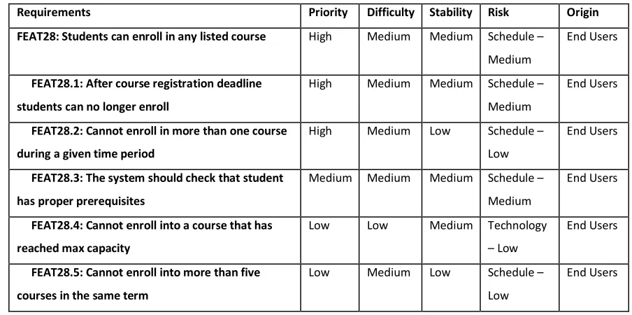
Table 1-1 is an example for a textual functional requirement in a University Course
Online Registration System project written using the RequisitePro tool. In this example,
the main functional requirement is FEAT28 and there are five sub-requirements which
Table 1-1 Functional Requirement Example
Requirements Priority Difficulty Stability Risk Origin
FEAT28: Students can enroll in any listed course High Medium Medium Schedule –
Medium
End Users
FEAT28.1: After course registration deadline
students can no longer enroll
High Medium Medium Schedule –
Medium
End Users
FEAT28.2: Cannot enroll in more than one course
during a given time period
High Medium Low Schedule –
Low
End Users
FEAT28.3: The system should check that student
has proper prerequisites
Medium Medium Medium Schedule –
Medium
End Users
FEAT28.4: Cannot enroll into a course that has
reached max capacity
Low Low Medium Technology
– Low
End Users
FEAT28.5: Cannot enroll into more than five
courses in the same term
Low Medium Low Schedule –
Low
End Users
With respect to the functional requirement listed in Table 1-1, the main requirement
FEAT28 is mapped to a use case named ―Enroll a Course‖. The sub-requirement
FEAT28.1 describes three main transactions. The first transaction is that the student
should select the course he or she wishes to enroll in. This is mapped to a transaction in
the Success scenario. The second transaction is that student enrolls in the course which is
also a transaction in the success scenario. The third transaction describes a condition that
students should register before the deadline which should be listed under the Extensions
(Alternative Scenario). The sub-requirement FEAT28.2 states a condition that students
cannot enroll in two or more courses that run on the same time period. FEAT28.2 should
be treated as a transaction under the Extensions. FEAT28.3 is mapped to a transaction in
the Extensions scenario which checks if the prerequisites of the course are fulfilled.
Scenario) to describe the condition if the course prerequisites are not satisfied. FEAT28.4
describes a condition to check the maximum capacity of a course, which will be mapped
to a transaction under the Extensions. Finally, FEAT28.5 also states a condition to check
the number of courses registered by a student. Based on the above mapping description,
the use case description (aka use case scenario) of the use case ―Enroll a course‖ is
presented in Table 1-2.
Table 1-2 Use case description
Use Case Title: Student Enrolls in a Course
Actors: Student, Admin
Precondition: The student is not enrolled in a course
Main Success Scenario (Main Flow):
1. The student chooses the course he or she wishes to enroll in 2. The student enrolls in the course
Extensions (Alternative)
2a: The student does not have permission (e.g. the student has not paid the tuition) 2a1: Notify the student to contact the administrator
2b: The deadline has passed
2b1: An error message will be displayed 2c: The prerequisite of the course is not fulfilled
2c1: The student is advised to contact the professor to obtain permission 2d: Two courses have the same schedule
2d1: The student is advised to choose one or the other 2e: The number of the enrolled courses has been exceeded
2e1: An error message will be displayed 2f: The course is full
2f1: An error message will be displayed
1.2
Research Questions
This research focuses on predicting software effort from use case diagrams. The use case
point model [7] was the first model to deal with software effort prediction from use case
diagrams. There are many limitations to the use case point model such as the complexity
weights assigned to use cases and the description of these weights are not satisfactory,
and the weights of the technical and environmental factors are outdated. There is several
related work that addressed the issues of the use case model. Authors in [8] and [9]
worked on adjustment factors, while others in [9] and [10] highlighted the discrepancies
in designing use case models. Researchers in [11], [12] and [13] proposed different size
metrics such as Transactions, TTPoints and Paths, while others [14], [15], [16], [17],
[18], [19] and [20] went further to extend the UCP model by providing new complexity
weights or by modifying the method used to predict effort.
Based on the above literature, we highlighted some research gaps. First, none of the
above work used neural network models to predict software effort from use case
diagrams. Second, the above work used linear regression for software effort estimation.
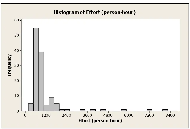
Third, the size of the projects used in most datasets is small (less than 4,000
person-hours). As well, the influence of non-functional requirements was not addressed
adequately. Thus, we ask seven relevant questions:
1. How can we measure the size of a use case and how can we estimate the size of a
use case diagram?
3. To what degree can software effort estimation be influenced by project
complexity?
4. How will unstable requirements affect the accuracy of software effort estimation?
5. To what degree can software effort prediction from use case diagrams be affected
by non-functional requirements (productivity, complexity and requirements
stability combined)?
6. What is the nature of the relationship between software effort and size?
7. What type of models can be used to predict software effort from use case
diagrams?
Regarding the first question, we conducted two experiments. In the first experiment
described in Chapter 3, we used the method proposed by the use case point (UCP) model
(this model is described in Chapter 2). We found that this model is inadequate,
specifically regarding large use cases. In the second experiment, which is presented in
Chapter 4, we proposed a new method to calculate the size of a use case, and
consequently the size of the use case diagram.
The second question is addressed in Chapters 3 and 4. In Chapter 3, we used the
environmental factors with their default weights proposed by the UCP model to calculate
productivity. However, these factors were filtered and new weights were proposed in
Chapter 4. Moreover, we used a fuzzy logic technique to calibrate the proposed
The third question is tackled in Chapter 4, as we proposed a new method to calculate the
complexity of a project.
The fourth question is addressed in Chapter 3 and Chapter 4. In Chapter 3, we used
requirements stability as one of eight factors that contribute to productivity. However, we
found that the requirements stability factor plays an important role in estimating software
effort. For this reason, we eliminated the requirements stability factor from the eight
factors that contribute to productivity and proposed requirements stability as one of the
independent factors that affect software estimation, which is also presented in Chapter 4.
The fifth question deals with the influence of non-functional requirements (NFR) on
software estimation. Many published work ignore the impact of NFR on effort
estimation. The UCP model [7] states that the NFR can increase the effort by about 30%.
However, others argue that NFR can represent more than 50% of the total effort [21].
This indicates that NFR can double the predicted effort. In our research, we found that
NFR can increase software effort by a factor of 2.6 (160%). In our model, we represent
NFR through three main factors, which include productivity, complexity and
requirements uncertainty. The productivity factor itself can increase the effort by 42%
which corresponds to the lowest degree of team productivity. However, the complexity
factor and requirements stability factors can increase software effort by 30% and 40%,
respectively which correspond to the highest complexity degree and to the highest
requirements uncertainty factors (this combination represents the NFR), the effort can be
increased to a factor of 2.6 (1.42*1.3*1.4) or by 160%.
In research question six, we ask about the relationship between software size and effort.
All researchers agree that software effort is correlated to software size. This means, when
software size increases, software effort will increase. However, many models including
the UCP claim that the relationship between software effort and size is linear. Other
prominent cost estimation models such as COCOMO claims that this relationship is
log-linear and it is represented asEfforta Size* b. In Chapters 3 and 4, we argue that this
relationship is non-linear. Specifically, we introduced three types of non-linear models in
Chapter 4 and we showed by experiments that these models outperform the log-linear
model especially for large projects. This is a breakthrough in the field of software
estimation.
In question seven, we investigate different models to see which one is suitable for
software effort prediction from use case diagrams. We show in Chapters 3 and 4 that
linear and non-linear regression models can be used for software effort estimation.
Furthermore, we assert that neural network models and especially MLP, RBFNN and
GRNN can also be used as alternatives to regression models. In Chapter 5, we present a
Treeboost model to predict software effort from use case diagrams based on three
1.3
Research Contributions
This thesis focuses on creating a model to predict software size and effort from use case
diagrams. Research contribution can be mainly summarized as follows:
1- Several experiments were conducted to figure out the nature of the relationship
between software effort and size. Results concluded that this relationship is
non-linear, although the degree of non-linearity varies based on how large the software
size is. For instance, this non-linear relationship is insignificant with small
projects. However, this non-linearity becomes evident with mid-sized projects and
stands out with large projects.
2- Six different levels of complexity for use cases were identified. These include
Very Low, Low, Normal, High, Very High and Extra High. This classification is
based on the number of transactions of each use case by giving the Success
scenario more weight than the Extension scenario.
3- A new method to calculate the productivity of the team developing a project was
proposed. The overall productivity factor is based on five factors; each has five
levels (Level-1 which corresponds to very low, to Level-5 which corresponds to
very high). These factors include team experience about the problem domain,
team motivation, experience in the programming language used, experience in the
object oriented language and the level of the analytical skills of the team.
Additionally, we propose a weight to each of these five factors that contribute to
of the five factors. Furthermore, we used a fuzzy logic technique to calibrate the
proposed productivity factor.
4- A new method to calculate the project complexity factor was put forward based
on five levels. A weight was assigned to each complexity level.
5- Five levels of requirements uncertainty were proposed. Requirements uncertainty
includes the increase in the number of requirements as well as the change of the
requirements during the software development life cycle.
6- Six different models were put forward to estimate software effort from software
size, productivity, complexity and requirements uncertainty. These models
include linear regression, non-linear regression, Multilayer Perceptron neural
network, Radial Basis Function Neural Network, General Regression Neural
Network and Treeboost. Four experiments were carried out to evaluate and test
the proposed models with two other models that conduct software estimation from
use case diagrams. In the first experiment, all models were tested using 65 data
points of effort ranging between 120 person-hours and 224,890 person-hours.
After that, the 65 testing data points were divided into three categories: Small
Dataset, which contains 25 projects of effort ranging between 120 person-hours
and 3,000 person-hours; Medium Dataset which contains 21 projects of effort
ranging between 3,000 person-hours and 10,000 person-hours; and Large Dataset
which contains 19 projects of effort greater than 10,000 person-hours. In the
second experiment, all models were tested using the Small Dataset; however, in
the Large Datasets respectively. A thorough comparison among all models was
carried out based on each experiment and recommendations on how to use each
model were proposed. Additionally, the proposed model was evaluated against
models that conduct software estimation from use case diagrams. The
experiments show that the proposed model outperforms other models based on
different evaluation criteria.
1.4
Thesis Structure
This thesis is organized as follows. Chapter 2 defines the terms used in this work, and
then presents a literature review, followed by related work. Chapter 3 introduces the
linear regression model and the Multilayer Perceptron neural network model. In Chapter
4, we elaborate on the linear and non-linear regression models, as well as the Radial
Basis Function Neural Network model and the General Regression Neural Network
Model. Chapter 5 proposes a Treeboost model to estimate software effort based on three
References
[1] J. Lynch. Chaos manifesto. The Standish Group. Boston. 2009[Online]. Available:
http://www.standishgroup.com/newsroom/chaos_2009.php.
[2] O. Demirors and C. Gencel, "A Comparison of Size Estimation Techniques Applied
Early in the Life Cycle," Software Process Improvement, vol. 3281, pp. 184-194, 2004.
[3] G. Kotonya and I. Sommerville, Requirements Engineering: Processes and
Techniques. Chichester; New York: John Wiley, 1998.
[4] D. Eck, B. Brundick, T. Fettig, J. Dechoretz and J. Ugljesa, "Parametric estimating
handbook," The International Society of Parametric Analysis, Fourth Edition. 2009.
[5] I. Jacobson, M. Christerson, P. Jonsson and G. Overgaard, Object-Oriented Software
Engineering: A use Case Driven Approach. Addison Wesley, 1992.
[6] J. Rumbaugh, I. Jacobson and G. Booch, "Use cases," in UML Distilled, 3rd ed., M.
Fowler, Ed. Pearson Higher Education, 2004, pp. 103.
[7] G. Karner, "Resource Estimation for Objectory Projects," Objective Systems, 1993.
[8] S. Diev, "Use cases modeling and software estimation: applying use case points,"
[9] B. Anda, H. Dreiem, D. I. K. Sjoberg and M. Jorgensen, "Estimating software development
effort based on use cases-experiences from industry," 4th International Conference on the Unified
Modeling Language, Modeling Languages, Concepts, and Tools, 2001, pp. 487-502.
[10] M. Arnold and P. Pedross, "Software size measurement and productivity rating in a
large-scale software development department," in Proceedings of the 20th International
Conference on Software Engineering, 1998, pp. 490-493.
[11] G. Robiolo and R. Orosco, "Employing use cases to early estimate effort with simpler
metrics," Innovations in Systems and Software Engineering, vol. 4, pp. 31-43, 2008.
[12] G. Robiolo, C. Badano and R. Orosco, "Transactions and paths: Two use case based
metrics which improve the early effort estimation," in International Symposium on
Empirical Software Engineering and Measurement, 2009, pp. 422-425.
[13] M. Ochodek and J. Nawrocki, "Automatic transactions identification in use cases,"
in Balancing Agility and Formalism in Software Engineering, B. Meyer, J. R. Nawrocki
and B. Walter, Eds. Berlin, Heidelberg: Springer-Verlag, 2008, pp. 55-68.
[14] K. Periyasamy and A. Ghode, "Cost estimation using extended use case point model," in
International Conference on Computational Intelligence and Software Engineering, 2009.
[15] F. Wang, X. Yang, X. Zhu and L. Chen, "Extended use case points method for
software cost estimation," in International Conference on Computational Intelligence
[16] G. Schneider and J. P. Winters, Applied use Cases, Second Edition, A Practical
Guide. Addison-Wesley, 2001.
[17] M. R. Braz and S. R. Vergilio, "Software effort estimation based on use cases," in
COMPSAC '06, 2006, pp. 221-228.
[18] A. B. Nassif, L. F. Capretz and D. Ho, "Estimating software effort based on use case
point model using sugeno fuzzy inference system," in 23rd IEEE International
Conference on Tools with Artificial Intelligence, Florida, USA, 2011, pp. 393-398.
[19] P. Mohagheghi, B. Anda and R. Conradi, "Effort estimation of use cases for
incremental large-scale software development," in Proceedings of the 27th International
Conference on Software Engineering, St. Louis, MO, USA, 2005, pp. 303-311.
[20] M. Ochodek, J. Nawrocki and K. Kwarciak, "Simplifying effort estimation based on
Use Case Points," Information and Software Technology, vol. 53, pp. 200-213, 2011.
[21] Y. Ossia. IBM haifa research lab. IBM Haifa Research Lab [Online]. 2011.
Available: https://www.research.ibm.com/haifa/projects/software/nfr/index.html.
Chapter 2
2.
Background
In this chapter, we define the terms used in this thesis such as fuzzy logic, neural network
and its types, as well as the criteria used to evaluate our work. Moreover, a literature
review and the related work are presented.
2.1
Fuzzy Logic
Fuzzy logic is derived from the fuzzy set theory that was proposed by Lotfi Zadeh in
1965 [1]. As a contrary to the conventional binary (bivalent) logic that can only handle
two values True or False (1 or 0), fuzzy logic can have a truth value which is ranged
between 0 and 1. This means that in the binary logic, a member is completely belonged or
not belonged to a certain set, however in the fuzzy logic, a member can partially belong
to a certain set. Mathematically, a fuzzy set A is represented by a membership function as
follows:
[ ] ( ) : [0,1].
z A
F xA x (2.1)
Where A is the degree of the membership of element x in the fuzzy set A.
A fuzzy set is represented by a membership function. Each element will have a grade of
membership that represents the degree to which a specific element belongs to the set.
linguistic variables are used to express a rule or fact. For example, ―the temperature is
thirty degrees‖ is expressed in fuzzy logic by ―the temperature is low‖ or ―the
temperature is high‖ where the words low and high are linguistic variables. In fuzzy
logic, the knowledge based is represented by if-then rules. For example, if the
temperature is high, then turn on the fan. The fuzzy system is mainly composed of three
parts. These include Fuzzification, Fuzzy Rule Application and Defuzzification.
Fuzzification means applying fuzzy membership functions to inputs. Fuzzy Rule
Application is to make inferences and associations among members in different groups.
The third step in the fuzzy system is to defuzzify the inferences and associations, make a
decision and provide an output that can be understood. In this thesis work, fuzzy logic is
used to calibrate the productivity factor of the regression model.
2.2
Neural Network
Artificial Neural Network (ANN) is a network composed of artificial neurons or nodes
which emulate the biological neurons [2]. ANN can be trained to be used to approximate
a non-linear function, to map an input to an output or to classify outputs. There are
several algorithms available to train a neural network but this depends on the type and
topology of the neural network. The most prominent topology of ANN is the
feed-forward networks. In a feed-feed-forward network, the information always flows in one
direction (from input to output) and never goes backwards. An ANN is composed of
weighted inputs are aggregated, thresholded and inputted to an activation function to
generate an output of that node. Mathematically, this can be represented by:
0 1
( ) [ ].
n i i i
y t f w x w
(2.2)Where xi are neuron inputs, wi are the weights and f[.] is the activation function. There
are many types of activation functions as shown in Figure (2-1) [3].
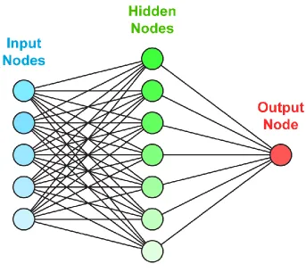
Feed-Forward ANN layers are usually represented as input, hidden and output layers. If
the hidden layer does not exist, then this type of the ANN is called perceptron. The
perceptron is a linear classifier that maps an input to an output provided that the output
falls under two categories. The perceptron can map an input to an output if the
relationship between the input and output is linear. If the relationship between the input
and output is not linear, one or more hidden layers will exist between the input and output
layers to accommodate the non-linear properties. Several types of feed-forward neural
networks with hidden layers exist. These include Multilayer Perceptron (MLP), Radial
Basis Function Neural Network (RBFNN) and General Regression Neural Network
(GRNN).
2.2.1
Multilayer Perceptron (MLP)
A MLP is a feed-forward neural network model that contains at least one hidden layer
and each input vector is represented by a neuron. The main difference between the MLP
and the Perceptron is that in the Perceptron, there are no hidden layers. In general, the
neurons in the hidden layer use non-linear activation function such as the sigmoid
function (logistic). The output layer node usually uses a linear activation function. The
number of hidden neurons varies and can be determined by trial and error so that the error
is minimal. MLPs are usually trained using the backpropagation algorithm which is a
type of gradient decent algorithm. Another algorithm can be used to train a MLP which is
the conjugate gradient algorithm [4]. The applications of the MLP model include image
the schematic diagram of a MLP that has five input vectors, seven neurons and one
output.
Figure 2-2 Schematic diagram of a MLP model
2.2.2
Radial Basis Function Neural Network
A Radial Basis Function Neural Network (RBFNN) was introduced by Broomhead and
Lowe [5]. A RBFNN is a feed-forward network that has three layers; an input layer, a
Figure 2-3 Schematic diagram of a RBFNN model [5]
The first layer is the input layer that represents the input vectors (in this chapter, there are
four input vectors; software size, team productivity, project complexity and requirements
stability). The hidden layer contains a set of neurons that use Radial Basis Function
(RBF) as activation functions. An RBF function depends on the distance from its center
Ci to the input X. Each RBF function has a radius or width (also called spread) which is
denoted by ― ‖. The width might be different for each neuron. The Gaussian function is
the most commonly used in RBF as shown in Equation (2.3):
2
2
( ) exp( ).
2
i i
X C
f x
(2.3)
Where Ci is the center and iis the width of the ith neuron in the hidden layer. The
of the RBFNN over other feed-forward neural networks include fast learning and not
suffering from problems such as local minima and paralysis [6].
2.2.3
General Regression Neural Network
The General Regression Neural Network (GRNN) is a type of neural networks that
performs regression on continuous target (output) variables. The GRNN was proposed by
Specht in 1991 [7]. A GRNN is composed of four layers as depicted in Figure (2-4).
Figure 2-4 Schematic diagram of a GRNN model [7]
The first layer is the input layer in which each independent variable (predictor) has a
The second layer contains pattern neurons such that each training row in the training
dataset has a neuron. Each neuron computes the Euclidean distance from the input vector
X to the neuron’s center, then applies the RBF function using the sigma ― ‖ values. The
resulting value is then passed to neurons in the third layer (summation neurons).
The third layer only contains two neurons. One neuron is called the denominator
summation which adds the values of the weights coming from each of the pattern neurons
(second layer). The other neuron is the numerator summation that adds the weights
multiplied by the actual output (target) value of each pattern neurons.
The fourth layer contains the output neuron in which the value stored in the numerator
neuron is divided by the value stored in the denominator neuron. The output is the
predicted target value.
The GRNN has several advantages such as they learn faster and are more accurate than
other neural network models. Moreover, GRNN models are fairly insensitive to outliers.
The main disadvantage of GRNN is that it requires more memory space to store the
model and it becomes inapplicable if the number of the training project datasets is very
huge.
2.3
Evaluation Criteria
Several methods exist to compare cost estimation models. Each method has its
advantages and disadvantages. In our work, five different evaluation methods have been
Mean of Magnitude of error Relative to the Estimate (MMER) the Prediction Level
(PRED), the Mean Error at 95% Confidence Interval (CI) and the Mean Absolute Error
(MAE).
MMRE: This is a very common criterion used to evaluate software cost
estimation models [8]. The Magnitude of Relative Error (MRE) for each
observation i can be obtained as:
| |
.
i i
i
i
Actual Effort Predicted Effort
MRE
Actual Effort
(2.4)
MMRE can be achieved through the summation of MRE over N observations:
1 1 . N i MMRE MRE N
(2.5) MMER: Another method can be used as an alternative to the MMRE which is the
Magnitude of Error Relative to the estimate (MER) [9]. MER is similar to MRE
with a difference that the denominator is the predicted effort instead of the actual
effort. Consequently, the equations for MER and MMER are:
| |
.
i i
i
i
Actual Effort Predicted Effort
MER
Predicted Effort
(2.6)
1 1 . N i MMER MER N
(2.7)As seen from Equations (2.4) and (2.6), improving one method might adversely affect the
denominator of MER is the predicted effort. Nevertheless, it is important that MMRE and
MMER are both used for evaluation. For instance, if the MMRE is large and the MMER
is small, this indicates that the average actual effort of the projects is less than the average
estimated effort. On the contrary, large MMER values indicate that the average estimated
effort is less than the average actual effort.
PRED(x): PRED (x) can be described as:
. kPRED x n
(2.8)
where x is the maximum MMRE (or MMER) of a selected range, n is the total number of
projects, and k is the number projects in a set of n projects whose MMRE (or MMER) <=
x. PRED calculates the ratio of a project’s MMRE (or MMER) that falls into the selected
range (x) out of the total projects. For example, PRED (30) gives the percentage of
software projects that were estimated with MMRE (or MMER) less than or equal to 0.3.
The estimation accuracy is proportional to PRED (x) and inversely proportional to
MMRE or MMER.
CI: The equation of the mean error confidence interval is:
* SD .
CI x t
N
(2.9)
Where xis the mean error, SD is the standard deviation, N is the number of projects and t
is a constant called the test statistic that depends on the number of the samples (projects)
table. The 95% confidence level becomes standard to many disciplines. For example, the
value of t is 2.042, 2, 1.98 and 1.96 if the number of projects is 30, 60, 100 and 1,000
respectively at the 95% confidence level. For instance, the value (SD/√N) is called the
standard error of the mean.
The equation for the mean error for each observation i and total number of observations
N is: 1 . 1 N i i x x N
(2.10)Where xi (Actual Effort iPredicted Efforti)
The equation of the standard deviation can be seen as:
2 1 1 ( ) . 1 N i i
SD x x
N
(2.11) MAE: The Mean Absolute Error (MAE) is the average of the absolute errors
between the actual and the predicted effort as shown in Equation (2.12).
1 1 | | . N a p i
MAE E E
N
(2.12)Where Ea is the actual effort and Ep is the predicted effort.
2.4
Literature Review
Software estimation can be affected by several parameters [10] . These parameters
Size: The effort and cost of a software project depends on the size of the project.
The larger the size is, the higher effort and cost will be needed. Software size
estimation will first be performed if the size of the project is unknown upon
conducting effort estimation. The size of a project can be measured in Source
Lines of Codes (SLOC) or Function Points (FP).
Category: The category of a project is important in software estimation. Examples
of project categories include Development, Maintenance, Migration, etc.
Personnel Attributes: The experience and the productivity of a team affect
software estimation.
Domain: The domain of the project might affect software estimation. The effort to
build a human resources management system is different from the effort needed to
develop an accounting and stock management system. Examples of domain
categories include finance, insurance, retail and manufacturing.
Complexity: the complexity of a project plays an important role in software
estimation. Examples of complexity include mission-critical (will the application
be used in a healthcare system to monitor the heartbeats and the blood pressure of
a person?), architecture (is the architecture 2 tiers, 3 tiers or multi-tiers?) and
Service Level Agreement (will there be a strict SLA that should be met?).
There are several models for software effort and cost estimation. These include
algorithmic models, expert judgement models, estimation by analogy models and soft
2.4.1
Algorithmic Models
This is still the most popular category in the literature [11]. These models include
COCOMO [12], SLIM [13], Function Point, Use Case Points [20] and SEER-SEM [14].
The main cost driver of these models is the software size. In COCOMO and SLIM
models, the size is measured in Source Lines of Code (SLOC). However, the function
point and the use case point models take software size in function points (FP) and use
case points (UCP) respectively. Algorithmic models either use a linear regression
equation, the one used by Kok et al. [15] or non-linear regression equations, those which
are used by Boehm [12].
2.4.1.1 COCOMO
The COnstructive COst MOdel (COCOMO) is an algorithmic model used to predict
software cost. It was developed by Barry Boehm in 1981 [12], and it was known as
COCOMO 81. COCOMO uses a simple regression formula. The model’s parameters are
derived from historical projects and current project characteristics. There are three main
types of COCOMO 81. These include Basic COCOMO, Intermediate COCOMO and
Detailed COCOMO. The Basic COCOMO equations are as follow:
.
b
Effort a Size (2.13)
Where Effort is measured in person-months and Size is measured in KSLOC. The
constants ―a‖ and ―b‖ are determined based on the project type as seen in Table (2.1).
_ d.
Development Time c Effort (2.14)
Where Development_Time is measured in months. The constants ―c‖ and ―d‖ are also
shown in Table (2.1). Equation (2.15) shows the number of people required for the
project development.
_ Re .
_ Effort
People quired
Development Time
(2.15)
The constants ―a‖, ―b‖, ―c‖ and ―d‖ are determined based on three categories of projects
which are Organic, Semi-detached and Embedded as shown in Table (2-1). Organic
projects are projects where small teams with good experience are working with non-strict
requirements. Projects are classified as Semi-detached when medium teams with mixed
experience are working with requirements which are mixed between strict and non-strict.
Embedded projects are those that have tight constraints.
Intermediate COCOMO is an advanced model of the Basic COCOMO where software
effort is a function of software size and 15 other cost-driver attributes. These attributes
represent the non-functional requirements of the project. Each attribute has a rate on a
six-point scale ranging from ―very low‖ to ―extra high‖.
Detailed COCOMO incorporates the characteristics of the Intermediate COCOMO with
Table 2-1 Software project types [12]
Software Project a b c D
Organic 2.4 1.05 2.5 0.38
Semi-detached 3.0 1.12 2.5 0.35
Embedded 3.6 1.20 2.5 0.32
Boehm introduced COCOMO II model [16] which is an advanced model of COCOMO
81. COCOMO II is more suitable for estimating modern software development projects.
The main differences between COCOMO II and COCOMO’81 can be summarized as:
COCOMO II takes into account requirements volatility.
Estimation is adjusted for software reuse and re-engineering when automated
tools are used.
Cost drivers were updated.
COCOMO II has more data points (161 data points as opposed to 63 in
COCOMO’81.
COCOMO II uses logical SLOC where COCOMO’81 uses physical SLOC. One
logical SLOC (if-then-else) might contain several physical SLOC.
2.4.1.2 SLIM
The Software LIfecycle Management (SLIM) model, which is also known as the Putnam
model was developed by Lawrence Putnam in 1978 [13]. The SLIM describes the effort
follows the Rayleigh distribution as shown in Figure (2-5). The effort required to develop
a project is as follows:
3
4/3 .
Pr
Size
Effort B
oductivity Time
(2.16)
Where Effort is measured in person-years and Size in SLOC. Productivity is the process
productivity which is the ability of a software organization to develop software of a given
size at a certain defect rate. Time is measured in years where B is a scaling factor and it is
a function of project size.
2.4.1.3 Function Point Model
Function Points measure the functionality of software as opposed to SLOC which
measures the physical components of software. The function point method was proposed
by Allan Albrecht in 1979 [17] [18]. There are a few methods to count function points
but the standard method is the one that is maintained by the Function Points Analysis
(FPA) which is based on the International Function Point Users Group (IFPUG) [19].
FPA defines five parameters that the size of software depends on. These parameters
include inputs, outputs, inquiries, internal files and external interfaces. It is clear that
these parameters are touchable by the end user. Figure (2-6) shows the function points
parameters within an application [18]. These parameters are discussed as the following:
Inputs: These are inputs from the user to the application. For example, create,
delete, update and read are considered as inputs.
Outputs: This is an output of a certain process in the application. For example a
financial report in an organization. The financial report is considered as an output
if it is printed, or stored in a database or external media storage, or even if it is just
displayed on the screen.
Inquiries: These are queries executed by the user to fetch some data stored in the
database. The output of an inquiry is similar to the output discussed above, except
that business information is not processed in this case. Information is sorted or
Internal files: These files store all the data of the application. Internal files belong
to the application and are maintained by the application owner or the
administrator.
Interfaces: This is the interface of external applications by which transactions can
be made to the main application. The function point model defines interface as
files that belong to external applications and are supported by those applications,
however these files contribute to the size of the main application. For example,
the main application might request a file that contains important information and
this file is maintained and updated by other applications.
Users Internal Logical Files Measured Application External Interface Files Application Boundary Other Applications Internal Logical Files External Inputs External Outputs External Inquiries External Inputs External Outputs External Inquiries
Figure 2-6 High level view of the function point model
2.4.1.4 Use Case Point Model
The Use Case Point (UCP) model [20] is based on mapping a use case diagram to a size
metric called use-case points. A use case diagram shows how users interact with the
functional requirements where an actor is a role played by a user. Figure (1-2) is an
example of a use case diagram. Each use case is represented by a use case scenario
(description). The use case scenario (description) is mainly composed of a Success
scenario and an Extension (Alternative) scenario as shown in Table (2-2).
The use case point model was first described by Gustav Karner in 1993 [20]. This model
is used for software cost estimation based on the use case diagrams. First, the software
size is calculated according to the number of actors and use cases in a use case diagram
multiplied by their complexity weights. The complexity weights of use cases and actors
are presented in tables (2-3) and (2-4) respectively.
As shown in Table (2-3), the complexity of a use case is determined by the number of its
transactions as shown in the use case description of each use case. The software size is
calculated through two stages. These include the Unadjusted Use Case Points (UUCP)
and the Adjusted Use Case Points (UCP). UUCP is achieved through the summation of
the Unadjusted Use Case Weight (UUCW) and Unadjusted Actor Weight (UAW).
Table 2-2 Use case scenario (description)
Use Case Title: Student Enrolls in a Course
Actors: Student, Admin
Precondition: The student is not enrolled in a course
Main Success Scenario (Main Flow):
1. The student chooses the course he or she wishes to enroll in 2. The student enrolls in the course
Extensions (Alternative)
2a: The student does not have permission (e.g. the student has not paid the tuition) 2a1: Notify the student to contact the administrator
2b: The deadline has passed
2b1: An Error message will be displayed 2c: The prerequisite of the course is not fulfilled
2c1: The student is advised to contact the professor to obtain permission 2d: Two courses have the same schedule
2d1: The student is advised to choose either one 2e: The number of the enrolled courses has been exceeded
2e1: An error message will be displayed 2f: The course is full
2f1: An error message will be displayed
Post condition: The student has enrolled in a course
Table 2-3 Complexity weights of use cases [20]
Use Case Complexity
Number of Transactions Weight
Simple Less than 4 (should be realized by less than 5 classes)
5
Average Between 4 and 7 (should be realized between 5 and 10 classes)
10
Complex More than 7 (should be realized by more than 10 classes)
15
Table 2-4 Complexity weights of actors [20]
Actor Complexity Description Weight
Simple Through an API 1
Average Through a text-based user interface 2
![Figure 1-2 Use case diagram [6] ](https://thumb-us.123doks.com/thumbv2/123dok_us/7794890.1292872/27.612.165.487.333.643/figure-use-case-diagram.webp)
![Figure 2-1 Activation functions [3] ](https://thumb-us.123doks.com/thumbv2/123dok_us/7794890.1292872/43.612.208.439.298.666/figure-activation-functions.webp)
![Figure 2-3 Schematic diagram of a RBFNN model [5] ](https://thumb-us.123doks.com/thumbv2/123dok_us/7794890.1292872/46.612.193.461.120.339/figure-schematic-diagram-of-rbfnn-model.webp)
![Figure 2-4 Schematic diagram of a GRNN model [7] ](https://thumb-us.123doks.com/thumbv2/123dok_us/7794890.1292872/47.612.201.454.319.596/figure-schematic-diagram-of-grnn-model.webp)
![Figure 2-5 Putnam’s time-effort graph based on Rayleigh distribution [13] ](https://thumb-us.123doks.com/thumbv2/123dok_us/7794890.1292872/56.612.153.496.358.615/figure-putnam-time-effort-graph-based-rayleigh-distribution.webp)
![Table 2-4 Complexity weights of actors [20] ](https://thumb-us.123doks.com/thumbv2/123dok_us/7794890.1292872/60.612.103.545.129.467/table-complexity-weights-actors.webp)