A toolbox for software optimization of QC-MDPC code-based cryptosystems

QC-MDPC code-based cryptosystems

Nir Drucker1,2 _{and Shay Gueron}1,2 1

University of Haifa, Israel 2

Amazon Web Services Inc., Seattle, WA, USA [email protected],[email protected]

Abstract. The anticipated emergence of quantum computers in the foreseeable future drives the cryptographic community to start consider-ing cryptosystems, which are based on problems that remain intractable even with strong quantum computers. One example is the family of code-based cryptosystems that relies on the Syndrome Decoding Prob-lem (SDP). Recent work by Misoczki et al. [34] showed a variant of McEliece encryption which is based on Quasi Cyclic - Moderate Density Parity Check (MDPC) codes, and has significantly smaller keys than the original McEliece encryption. It was followed by the newly proposed QC-MDPC based cryptosystems CAKE [9] and Ouroboros [13]. These motivate dedicated new software optimizations.

This paper lists the cryptographic primitives that QC-MDPC cryptosys-tems commonly employ, studies their software optimizations on modern processors, and reports the achieved speedups. It also assesses methods for side channel protection of the implementations, and their perfor-mance costs. These optimized primitives offer a useful toolbox that can be used, in various ways, by designers and implementers of QC-MDPC cryptosystems.

1

Introduction

Strong quantum computers are believed to emerge in some foreseeable future. Their potential existence threatens the security current public key cryptosys-tems that rely on the difficulty of factorization (e. g., RSA) and the discrete log problem (e. g., ECDSA/ECDH), and this has already driven the cryptographic community to start planning for new standardized cryptosystems [1]. Families of problems that are believed to provide an adequate basis for quantum safe cryptosystems are based on codes, lattices, hash functions, and multivariate polynomials. It is conceivable that future standards would include representa-tives from each family, as a safe strategy for the ecosystem. This paper focuses on code-based cryptography.

keys, and are therefore considered less practical (e. g., [12,29,39]). Introducing some structure to the codes, reduces the key sizes (e. g., [5,10,32]), but may also lead to some security issues (e. g., [14,36]). For example, Low Density Parity Check (LDPC) codes [15] can leverage the structure to improve performance and decrease the key sizes, but seem to be insecure (e. g., [4,6,7,35]).

A recent study by Misoczki et al. [33,34] suggests that using QC-MDPC codes with a McEliece encryption type cryptosystems enjoy relatively short keys (shorter than McEliece). However, as an encryption scheme, it was shown to be susceptible to an attack [24] by an adversary with some budget of chosen decryp-tion queries. The attack leverages the fact that there is some probability, termed (by [34]) Decoding Failure Rate (DFR), that the decoding may fail to compute the errors. Indeed, [24] showed that merely knowing if decoding failed with some adversary-crafted ciphertexts, allows the adversary to reveal the private key. Nevertheless, a corresponding Key encapsulate Mechanism (KEM) scheme can still be secure, if ephemeral public-private key pairs are used for each exchange, as proposed by the recent KEM scheme CAKE [9]. For 128=bits quantum se-curity, CAKE is estimated to have a DFR of 10−7_{. Ouroboros [13] is a different} QC-MDPC code based KEM scheme. It has the same parameters, almost the same decoding as MDPC McEliece, and a security reduction to decoding ran-dom quasi-cyclic codes in the Ranran-dom Oracle Model [3]. It also has a public key which is roughly 2xsmaller than that of CAKE and an estimated DFR varying between 10−5 _{to 10}−7 _{(depending on the parameters).}

The proposed QC-MDPC codes McEliece-style encryption [33,34] sparked the study of the practical aspects of such cryptosystems, with a thorough study by Maurich et al. [30]. This comprehensive work covers a variety of optimiza-tions, from FPGA’s, lightweight architectures (IoT), ARMs Cortex-M4 micro-controller, and vectorization features of modern general-purpose x86 architec-tures, specifically for a) 80 bits classical security (FPGA/IoT/ARM); b) 40/64/ 128-bit quantum security (x86 platforms).

In this paper, we investigate general software optimizations for QC-MDPC codes cryptosystems, focusing mainly on 128 bits quantum security parameter as the primary motivation.

Our contribution. We study several software optimizations that leverage special features of modern processor architectures, and compare our results to those achieved in [30]. By listing the main primitives that are needed for the related protocols, we explain these software optimizations can be used (beyond the McEliece-type encryption) for general QC-MDPC codes cryptosystems, such as CAKE [9], and Ouroboros [13]. We show how different parameter choices af-fect the performance, demonstrate techniques for side channel protection of such implementations, and analyze their costs.

2

Preliminaries and notation

2.1 QC-MDPC

Letn, rbe positive integers. A binary (n, r) linear-codeCof lengthn, dimension k = n−r, and codimension r is a (n−r) dimension vector subspace of Fn2. It can be defined, equivalently, by either: 1) a generator-matrix G ∈ F₂k×n, where C = {mG ∈ Fn2|m ∈ Fk2}; 2) a parity check matrix H ∈ F

r×n 2 , where C={c∈Fn2|HcT = 0}. The syndromes∈Fr2 ofx∈Fn2 is defined by s=HxT, wheres= 0 iffx∈ C.

An (n, r)-linear code is called Quasi Cyclic (QC) if there exists an integer n0, such that every cyclic shift by n0 positions, of a codeword c ∈ C, is also a codeword in C. If n = n0p for some integer p ≥1, then both the generator and the parity-check matrices are composed of p×p circulant blocks. These matrices are uniquely defined by the first row of each circulant block. With such interpretation, this row can be viewed as a polynomial in_Fn

2[x]

(xr_{+ 1). These} equivalent interpretations are used hereafter interchangeably.

LDPC and MDPC codes are (n, r, w)-codes that are defined by a parity-check matrix where the Hamming weight of each row isw. Whilewis small for LDPC codes (e. g., less than 10), MDPC codes typically have w = O(pnlogn). An (n, r, w)-QC-MDPC code is an (n, r, w)-MDPC code that is QC where n=n0r (typically,n0= 2).

2.2 Choices of parameters

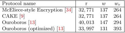
To illustrate the parameters’ range we are interested in, Table 1 shows a few QC-MDPC codes protocols choices, aiming at λ = 128-bit quantum security. Table 1 unifies the notation of [13,33,34] as follows:wis the weight of a sparse r-bits vector, and weis the weight of the error vector (their values are derived fromr andλ). The usage and rationale behind these choices, are given therein.

Protocol name r w we

McEliece-style Encryption [34] 32,771 137 264

CAKE [9] 32,771 137 264

Ouroboros [13] 40,013 147 294 Ouroboros (optimized) [13] 33,997 131 393

Table 1: Some QC-MDPC parameter choices that correspond to λ = 128-bit quantum security. Here, r defines an (2r, r)-code with 2 circulant blocks, w is the weight of a sparse vector, andwe is the weight of the error vector.

We also note that r needs to be a prime, and that it is convenient to also impose the following condition [9,34]: (xr_{+1)/(x+1) is an irreducible polynomial} (of degree r−1). This allows for efficient selection of an invertible element of F2[x]/(xr_{+ 1), by simply taking any polynomial with odd weight.}

2.3 Definitions and notation

QC-MDPC cryptosystems operate on polynomials inFr2

(xr+ 1). We view poly-nomials and strings of bits, interchangeably, as follows.

Definition 1 (Bit strings, polynomials.). A string is a finite sequence of bits (symbols in {0,1}). Letr >0 be an integer, and letA be a string of length

r, A=ar−1ar−2. . . a0, where, for 0 ≤j ≤r−1,aj is the bit in position j of A. We call ar−1 the most significant bit (of A) and a0 the least significant bit

(of A). By convention, the most significant bit is the bit in the leftmost position (in A), and the least significant bit is the bit in the rightmost position. LetA= ar−1ar−2. . . a0 be a string ofr bits, and let a(x) =ar−1xr−1+. . . a1x+a0 be

a (formal) polynomial of degree r−1. We view Aanda(x), interchangeably, as the same entity, depending on the context.

Example 1. The length of the string A = 10010100 is r = 8 (bits), a7 = 1, a6 = 0, a4 = 1, a2 = 1, a0 = 0. The polynomial a(x) = x7_+x4_+x2 _{can be} viewed (identified), interchangeably, as the stringA= 10010100.

For designing concrete QC-MDPC implementations, where the polynomials have degreer−1 and 86 |r, it is useful to embed the associated strings in arrays of bytes. This allows for conveniently carrying out some operations on the embedding arrays. If B is an array of sbytes, then itsjth _{byte (0≤j≤s−1) is denoted} by B[j]. By convention, values of bytes are hereafter written as (exactly) two hexadecimal digits.

Definition 2 (Embedding in an array of bytes.). Let A=ar−1ar−2. . . a0

be a string, where 86 |r. The following procedure embeds A in an array ofNB=

r/8

bytes,A¯ = ¯aNB−1¯aNB−2. . .a¯0. Writer= 8u+δwithu≥0 and0< δ <8.

Pad A, from the left, with 8−δ zero bits, so that it has 8(u+ 1) bits. Let A0

denote the result, i. e.,

A0=a0_8u+7. . . a0₀= 00. . .0 | {z } 8−δ bits

ar−1ar−2. . . a0

The bytes of Aare defined, bitwise, as ¯aj =A[k] =a0_8k+7. . . a0_8k, k= 0, . . . , u. We say that (the bits string) Ais embedded in (the array of bytes) A¯.

Example 2. The polynomialx20_+x16_+x2_{+x+ 1 corresponds to the bits string} 100010000000000000111 of length r = 21 bits. Write r = 21 = 8×2 + 5, pad A withδ = 8−5 = 3 zero bits, to 000100010000000000000111 (of 21 + 3 = 24 bits). Then,Ais embedded in the array ofNB=

21/8

Definition 3 (Redundant representation of strings of bits.). Let A = ar−1ar−2. . . a0be a string of bits. The redundant representation ofAis the array ˜

A, of rbytes, whereA[˜i] =01ifai= 1 andA[˜ i] =00otherwise, 0≤i≤r−1.

Example 3. LetAbe the string of bits 1011 (i. e., the polynomialA=x3_+x+1). Its redundant bytes representation isA˜ =01000101

Definition 4 (Blocks.). An array of 16bytes (a string of128 bits) is called a block. Every integer0≤j≤2128_{−1can be encoded as a block, which is denoted}

by encode128(j).

Example 4. encode128(256) =00000000000000000000000000000100. encode128(2128−5) =fffffffffffffffffffffffffffffffb.

Definition 5 (Leftwise cyclic rotation.). Let B be an array of sbytes and let0≤i≤s−1be an integer. The (leftwise) cyclic rotation ofB, byipositions, is the array rotl(B,i) of s bytes, where rotl(B,i)[j] = B[(i+j) (mods)], j = 0, . . . , s−1.

Example 5. Let A be the bytes array 11100100 of size 4. Then rotl(A,3) = 00111001

Finally, for two integers x1, x2, we define the function compare(x1, x2) to return a single bit: 1 if x1 = x2, and 0 otherwise, denote concatenation by k, and denote thej’s column ofH byhj↓.

3

The QC-MDPC based cryptographic primitives and

their optimizations

3.1 The cryptographic primitives

QC-MDPC code-based cryptosystems can be implemented with (combinations of) the following primitives.

1. A constrained pseudorandom bits stream generator: A PRF that uses a seed and generates a stream of bits that satisfies some constraints.

2. A hash function: used for compressing a sampled value of a random variable into a (short) seed/key.

3. Polynomial multiplication in_F2, and reduction moduloxr+ 1.

4. Decoding: an algorithm used for computing an unknown error from a given syndrome.

Note that some primitives (e. g., decoding) can be optimized ”unilaterally” by one of the protocol’s participants, and other optimizations (e. g., deriving a shared secret) need to be agreed at the protocol level, for interoperability. In addition, the cryptographic components themselves should the quantum safe (we useAES256, andSHA384)

3.2 Side channel considerations

We consider here two types of side channel adversaries that collect information on code that is executing on a given platform.

– Traffic analysis eavesdropper: this adversary has (passive) access to the net-work that the platform is using, and can collect timing information of dif-ferent steps of the protocol, based on the observed traffic.

– A spy program adversary: this adversary is running on the same platform, in parallel to the execution of the victim code, and at the same (or lower) privilege level. It can collect micro-architectural information such as memory access patterns and code and taken (not taken) branches.

We assume that both adversaries obtain their information with absolute accu-racy. This implies (for a traffic analysis eavesdropper) that the execution time of protocol steps, of a side channel protected code, should not reveal any secret in-formation, and for a spy program, that the timing, memory access patterns, and the branches of a protected code should not reveal secret information. For short, we call such protected code a ”constant time” implementation. Mitigation meth-ods against both adversaries are more expensive than mitigation against traffic analysis eavesdropper alone. Therefore, an implementation needs to choose the appropriate threat model that it needs to address.

3.3 A constrained pseudorandom bits stream generator

We handle three types of pseudorandom bits stream generation z ←− {0$ ,1}α (for an integerα >0): a) No constraints onz(Alg. 1); b)zhas odd weight (Alg. 2); c)z has weightw, for some a-priori prescribed weightw(Alg. 3).

An example for Algorithm 1 is given in Appendix B. Algorithm 2 is then self explanatory. We explain some details of Algorithm 3.

Generating a bit streamAwith a pre-defined weightw. This is equivalent to generating a list ofweightrandom positions (wlist) where the bits in the target string oflenbits are set. Each entry inwlistis an integer between 0 andlen. When log₂(len) is not an integer, as in the cases of interest here, we first consume a sample of b =

log₂(len)

bit from the AES-CTR-PRF. Note that reducing it modulolendoes not give a uniform random distribution (small values are more frequent). Therefore, Alg. 3 uses the rejection method: samples that are smaller thanlenare considered, and other samples are rejected (see also [30]). Since the rejection probability isp= 1−len

2b <

1

2, the expected number of samples needed to collect w valid values is at most 2w. Note that the rejection probability is larger whenlenis slightly larger thanb. For example, iflen= 32,771 = 215+ 3 then p ≈0.5, and if len = 32,749 = 215_{−19, p ≈0.0006. Sampling for cases} wherelenis not close to a power of two, is optimized in [23], as in the following example.

Example 7. Let w= 90,len= 9,602. Then, b=

log₂(len)

= 14,p= 0.41, so the expected number of samples (14 bits) is 90×1/0.59≈153 (153×14 = 2142 bits). However, choosing an upper bound of 3×len = 28,806 (a sample may require reduction modulo len), and consuming b = 15 pseudorandom bits at a time, gives a rejection rate ofp= 0.12, and reduces the expected number of such samples to 90×1/0.88 = 103 (103×15 = 1545 bits).

Side channel considerations for Algorithms 2 and 3. Alg. 2 runs in constant time, except for step 3. However, the information that step 3 reveals is not confidential. Alg. 3 generates awlist(in constant time), with set bit positions for the target string. However, na¨ıvely starting from a zero string and flipping the bits in the relevant positions (perwlist) is not secure against a spy program, because the memory access pattern may leak sensitive information (e. g., the secret key in CAKE and Ouroboros). To this end, we propose Alg. 4.

Algorithm 1 z=GenPseudoRand(seed,len) Input:seed(32 bytes)

Output:z(pseudorandom stream oflenbitsz embedded in an array of bytes). Exception:SeedOverUseError(seed overused).

1: procedureGenPseudoRand(seed,len) 2: s= AES-CTR-PRF-Initseed,0,232−1

3: z =truncatelen AES-CTR-PRF (s,len)

Algorithm 2 z=GenPseudoRandOddWeight(seed,len) Input:seed(32 bytes),len

Output:z(pseudorandom stream oflenbitsz with odd weight, embedded in an array of bytes).

Exception:SeedOverUseError(seed overused). 1: procedureGenPseudoRandOddWeight(seed,len) 2: z = GenPseudoRand(seed,len)

3: if weight(z) iseven then 4: z[0] = z[0]⊕1

5: returnz

Algorithm 3 wlist=GenPseudoRandWeightList(s,weight,len)

Input:s(AES-CTR-PRF state),weight(32 bits),len

Output:A list (wlist) ofweightbit-positions in [0, . . . ,len−1], updateds. Exception:SeedOverUseError(seed overused).

1: procedure_{GenPseudoRandWeightList}(s,weight,len)

2: wlist=φ

3: valid ctr= 0

4: whilevalid ctr<weightdo 5: (pos,s) = AES-CTR-PRF(s,4)

6: if ((pos<len) AND (pos6∈wlist))then

7: wlist=wlist∪ {pos}

8: valid ctr=valid ctr+ 1

9: returnwlist,s

Algorithm 4 A=ApplyWlist(wlist,len)

Input:A list (wlist) ofweightbit-positions in [0, . . . ,len−1]

Output:Aa stream oflenbitsAwith weightwembedded in an array of bytes. 1: procedureApplyWlist(wlist,len)

2: A[len:0] = 0

3: foriin 0. . .(len−1)do

4: forwinwlistdo

5: A[i] =A[i]BitWiseOr compare(i,w) 6: returnA

3.4 Efficient hashing

A cryptographic hash function is used as a one way function that generates a seemingly uniform random digest from a sampled random variable that has sufficient (min-)entropy. For efficiency, we use a parallelization technique that is designed to convert serial hashing to a parallelizable process (see [18,19,22]).

Lethash be a hash function with digest length of ld bytes. Suppose that it uses a compression function compress that consumes a block of size hbs bytes. Its associated ”parallelized hash”, ParallelizedHashhash

Algorithm 5 digest=ParallelizedHashhash

s,srem(array,la)

1: Input:an array oflabytesarray[la−1 : 0], such thatla≥s>0 2: Output:digest(ldbytes)

3: Context:hash,srem

4: procedureComputeSliceLen(la) 5: tmp :=jla

s

k −srem

6: α:=jtmp hbs

k

7: returnα×hbs+srem

8:

9: procedure_{ParallelizedHash}(array,la) 10: ls:= ComputeSliceLen(la)

11: lrem:=la- (ls×s) 12: fori:= 0 to (s-1)do

13: slice[i] =array[(i+ 1)×ls−1 :i×ls] 14: X[i] =hash(slice[i])

15: Y =array[la−1:ls×s]

16: YX=YkX[s−1]kX[s−2]. . . kX[0] 17: returnhash(YX)

The input to ParallelizedHash is an array of la bytes, array[la−1 : 0]. It is assumed that 0 <s ≤la. The array is split, logically, to s contiguous disjoint slices of equal (positive) length ls, and (potentially) a remainder buffer Y of lengthla−ls×sbytes (if this value equals 0, it means thatY is ignored). The length of a slice isls=α×hbs+srem where

α=      j

la s k

−srem

hbs    

 (1)

The slices are denotedslice[s−1],slice[s−2], . . . ,slice[0]. Thesslices are hashed, independently, andssub-digestsX[s−1], X[s−2], . . . , X[0] are computed, by

X[j] =hash(slice[j]) j = 0, . . . ,s−1 (2) Finally, the output ofParallelizedHashisdigest, where

digest=hash(Yk X[s−1]k X[s−2]k . . . k X[0]) (3)

A specific instantiation of ParallelizedHash. This paper uses

ParallelizedHashSHA384_8,111 . This implies ld= 48 andhbs= 128. A concrete example is given in Appendix C.

2 invocations of SHA384Update. The 8 (independent) slices can be hashed in parallel. This requires 2×8 = 16 parallelizable invocations of SHA384Update, generating 8 digests of 48 bytes, each. The remainder block has 2,000−239×8 = 88 bytes. Together with the 8 digests of the slices, the final step is hashing an array of bytes with 384 + 88 = 472 bytes. This requires 3 + 1 = 4 invocations of SHA384Update. The total number ofSHA384Updateinvocations of is 16+4 = 20. For comparison, note that the serialSHA384of 2,000 bytes, requires 16 serialized invocations of SHA384Update. However, on modern platforms, computing 20 calls toSHA384Update, of which 16 can be parallelized, can be optimized (using SIMD architectures), and be faster than 16 serial invocations ofSHA384Update.

Remark 1 (The choice of srem = 111). To motivate the choice srem = 111, compare it to the choices= 8 and srem= 0, applied to an array of la= 2,000 bytes. Here, ls= 128, lrem= 2,000−8×128 = 976. Therefore, the number of SHA384Updateinvocations is 8×2 + 8 = 24 (of which 16 can be parallelized). The number ofSHA384Updateinvocations withsrem= 111, is only 20.

3.5 Polynomial multiplication

Modern general-purpose processors are equipped with the ”carry-less multipli-cation” instruction PCLMULQDQ [20,21]: it computes the product of two bi-nary polynomials of degree 63. The operands of PCLMULQDQ are two xmm registers, an ”immediate” byte, and a destination register. The value of the im-mediate byte specifies which 64-bit halves (low/high) of the input registers are the multiplicands. The result, which is a polynomial of degree 126, is placed in the destination register. An appropriate software flow can usePCLMULQDQin order to multiply polynomials with any degree.

to revert to the schoolbook multiplication for the final step, as shown in the following example.

Example 9. For r = 4×64 a na¨ıve schoolbook algorithm uses 4×4 = 16 PCLMULQDQinstructions and 3×4 = 12 additions (XORs), and requires 8×64 bits of storage. A recursive Karatsuba calls itself three times with polynomials of degree 2×64−1 each call uses 3 PCLMULQDQ instructions and 5 XORs. This totals 9 PCLMULQDQ and 15 XORs, plus 10 extra XORs for the parent Karatsuba. The required memory is (8 + 2 + 4)×64 bits. On modern processors PCLMULQDQ has throughput 1 cycle and latency 7 cycles. When the school-book multiplication is pipelines (PCLMULQDQs invoked in parallel to XORs), it can theoretically end within 16 + 7 + 1 = 24 cycles (ignoring memory access overhead). On the other hand, a recursive Karatsuba would complete within 9 + 7 + 10 = 27 cycles (with more memory access overhead).

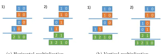
The final Schoolbook multiplication. We compare two methods, ”Horizon-tal” and ”Vertical”, for schoolbook multiplication of two polynomials p1, p2 of degreer−1, each one padded into aq=ceil((r−1)/64) 64-bit container. They are illustrated in Fig. 1.

1. Horizontal multiplication (a variant of this method is used in the gf2x library [37] that NTL library [38] users can choose to link): calculate p3[q : 0] = p1[0]×p2[q: 0]. Then, performp3[i+q:i] =p3[i+q:i]+ p1[:i]×p2[q: 0]

, fori= 1, . . . , q−1.

2. Vertical multiplication (our proposal): for 0 ≤ i, j, k ≤q−1, calculate (in parallel):

p3[2k+ 1 : 2k] = X

i+j=2k

p1[i]×p2[j]

Then, fork= 0, . . . , q−2, perform:

p3[2k+ 2 : 2k+ 1] =p3[2k+ 2 : 2k+ 1] + X i+j=2k+1

p1[i]×p2[j]

Polynomial reduction moduloxr+1inF2. Reducing a polynomialp∈F2[x] of degreer0,r≤r0≤2rmoduloxr+1 can be efficiently carried out by calculating p[r−1 : 0] = p[r−1 : 0]⊕p[r0 : r]. Software implementations on modern-processors can be vectorized by using AVX2/AVX512 extensions [26].

3.6 Decoding

(a) Horizontal multiplication (b) Vertical multiplication

Fig. 1: Schoolbook multiplication (2×2): Horizontal and Vertical. See details in the text.

vectorefromx, as the output. Note that other variants (e. g., in [13]) inherit the same general structure. Excluding the first syndrome calculation, Alg. 6 is built upon three repeated main steps: I) For i = 0, . . . , r−1, calculate the number of unsatisfied parity-checksupci (step 7); II) Find and compare the thresholds -fori= 0, . . . , r−1, flip the bit in positioni ofeifupci ≥τ for some threshold τ (steps 8-9); III) Addetoxand recalculate the syndromes(step 11). Steps I, II, III are repeated untils= 0 or until a maximal allowed number of iteration is attained, in which case the algorithm returns a ”decoding failure” flag.

Note that there are multiple options to chooseτ (the threshold that is used in Alg. 6), and they lead to different DFR and a different number of iterations (i. e., overall performance). Three examples are: 1) a predefined value as in [15]; 2) max

i upci as in [25]; 3) a small value below maxi upci as in [34].

In general, the decoding DFR and performance depend on multiple factors. This has led to various decoding algorithms, and new improved algorithms/-choices are still expected to emerge. We propose below separate optimizations for Steps I and III. Vectorization of Step II is straightforward. Consequently, our optimizations can be used by many variants of the BitFlip decoding algorithm.

BitFlip optimization. Maurich et al. [30] compare several decoders that do not require polynomial multiplications for updating the syndrome (Step III). They all take one of two approaches: a) When finding a bit j for which upcj > τ, flipe[j], update the syndrome tos=s+hj↓, and continue to the next bit. b)

Find and correct all the potential error bits ine, and update the syndrome to s=s+hj↓ for all the affected bits. The performance of a decoder that utilizes

the first approach, on an x86 platform, was reported in [30]. This implementation keeps a copy ofhj↓ in memory, and rotates and adds it (sometime masked) tos,

for each iteration. In this paper, we study decoders that use the second approach.

Optimizing Step I.: Alg. 7 shows our implementation of Step I. The inputs arewlist - a compact representation of hj↓ with windices, and˜s- a redundant

Algorithm 6 e=BitFlip(x,H)

Input:Parity-check matrixH∈Frxn2 ,x∈Fn2,maxIter(maximal # of iterations). Output:The errore∈Fn

2.

Assumption:A thresholdτ is either input or calculated dynamically. Exception:”decoding failure”

1: procedureBitFlip(x,H) 2: s =HxT_;

3: e = 0; 4: itr = 0;

5: while(s6= 0) and (itr<maxIter)do 6: fori in 0. . . n−1do

7: Computeupci .Step I

8: if upci> τ then

9: e[i] =e[i]⊕1 .Step II

10: itr = itr + 1

11: s =H(xT+eT) .Step III

12: if itr =maxIterthen 13: return”decoding failure” 14: returne

result of (up to 254) additions in each of the ˜s bytes. Note that in practice, w < 254 for QC-MDPC cryptosystems. The output of Alg. 7 is an array of bytes, U, where U[i] = upci. To speed up rotl(˜s,i), we duplicate ˜s in memory, into the duplicated syndrome ˜s×2 _{=˜sk˜s. The rotation rotl(˜s,i) is the memory} contents of the rbytes starting from the address of thei-th position, as shown in Fig. 2.

An implementation of Step I can choose two ways to compute the sum of upci, i= 0, . . . , r−1: a) Sum for each i separately (”Vertical”; b) sum for all i’s in parallel (”Horizontal”). Alg. 7) uses the Vertical summation. To explain why this approach is efficient on modern architectures, letM denote the overall number of bytes that can be stored in the processor’s wide-registers. Specifically, M = 29 bytes for AVX2, and M = 211 bytes for AVX512 architectures. When r > M, the array˜sis too large to fit in these registers. In this case, Horizontal summation needs to read, accumulate, and store intermediate results in some memory location (for each of thew iterations). This involves 2r memory reads plus r memory writes for each iteration - a total of 3wr memory operations. By comparison, Vertical summation accumulates the intermediate results in the wide registers, and stores them only in the end of each of the

r/M

iterations. This involvesw×M memory reads andM memory writes (for each iteration) -a tot-al of only 2w+M×

r/M

≈2wr/M memory operations. The difference becomes even more noticeable when 2r+M bytes do not fit in the last level cache of the processor, which is indeed the case for the typical QC-MDPC r values.

Fig. 2: rotl(˜s,i) example:˜s =˜s[3]k˜s[2]k˜s[1]k˜s[0]. Duplicating˜s in memory helps fast rotation (see explanation in the text)

.

Algorithm 7 U=CountUPC(˜s,wlist)

Input:˜s- a redundant representation ofrbits syndromes,wlist- awelements of the compact representation ofh0↓.

Output:U an array ofrbytes. 1: procedureCountUPC(˜s,wlist)

2: U=0

3: fori = 0, . . . , r−1do 4: forj = 0, . . . , w−1do

5: U[i] = U[i] +rotl(˜s,wlist[j])[i] 6: returnU

SIMD (AVX2 / AVX512) architectures, and parallelize part of the computations. To this end, it needs to operate on

r/M

chunks ofM bytes, and then handle the remainder ”tail” oftail=r−(r/M×M) bytes separately. We propose to avoid the cumbersome special handling by padding the duplicated syndrome˜s×2 (from the left) withM−tailadditional zero bytes, and working on the artificially longer array. Obviously, shorter padding leads to smaller overheads, and this makes some values ofrpreferable over other close values. For example, consider r = 32,771 = 215_{+ 3 (see Table 1), which is slightly above a multiple of M.} Padding˜s×2 _{to the next boundary ofM = 2}9_{bytes (for AVX2), or to M = 2}11 bytes (for AVX512) adds, respectively, 29_{−3 = 509 or 2}11_{−3 = 2,045 bytes.} By comparison, consider the close value r0 = 32,749 = 215_{−19 (smaller than} r by only 22), which is slightly below a multiple ofM. Here, the padding adds only 19 bytes. This is not saving only memory and memory accesses, but also saves one iteration of the algorithm. It can theoretically improve the performance by (32,771 + 2,045)/(32,749 + 19) = 1.06x. Similarly, r00= 32,719 = 215−49 (smaller thanrby only 52), requires padding of only 49 bytes, leading to savings in memory and computations. Remarkably, it turns out that r0 and r00, which are the two largest primes smaller than 215, also satisfy the requirement that (xr _{+ 1)/(x+ 1) is irreducible (The suggested value r}0 _{is due to P. S. L. M.}

Barreto).

r0₁= 22,511 = 214_{−17, which also satisfies the requirements. Here, the potential} speedup in the computations is (22,531 + 2,045)/(22,511 + 17) = 1.09x.

We point out that the performance gains from usingr0 orr00instead of using r, for QC−M DP C, should be weighed against the resulting DFR with these values. This DFR is reported in Section 4 (Table 3).

Reduced Weight optimization. We explore the following optimization, called hereafter ”Reduced Weight”, as an interesting tradeoff between performance and DFR: replace Step 4 of Alg. 7 fromfor j= 0, . . . , w dotofor j= 0, . . . , w−α do, for some nonnegative integer α. To not skip the same unsatisifed parity checks in each invocation of the algorithm, we rotateh0↓ (by a random index)

before using it. This reduces the number of iterations by α, and speeds up the CountUPCalgorithm by a factor of w/(w−α). For example, with w = 137 and α = 5, the speedup is 137/132 = 1.037x. This comes at the expense of a higher DFR because some parity checks are ignored. This is different from the optimization of [34], where all the unsatisfied parity checks are taken into account, and the threshold is max

i upci−δ. We note that the two optimizations can be applied simultaneously.

3.7 Constant time decoding

Constant time BitFlip. The BitFlip algorithm 6 handles the secret valuesH (input) ande, s(intermediate results). As a result, memory accesses, conditional execution, and latencies of operations can inadvertently leak information on the weights ofe,s. and on the positions of the set bits inH,e,s(e. g., through the number of errors fixed in a specific iteration and the number of iterations). A secure (”constant time”) implementation needs to prevent such potential leaks. Note that the number of iterations (either fixed of or variable) is implementation-dependent (e. g., [11]), and we keep it out of our scope.

CountUPC in constant time. The inputs of the CountUPC algorithm (Alg. 7) are H and s. A na¨ıve constant time implementation holds H in memory (entirely), and accesses it accordingly. Here, the required memory can be large: with n0 = 2 and 215 < r < 216 H occupies n0r2/23 > (228) ≈ 268 million bytes. The memory requirement can be reduced by storing onlyh0↓ in memory,

at the expense of some performance penalty (h0↓ needs to be rotated during

each of ther iterations). A different memory-performance trade off is obtained by duplicating h0↓ in memory, which speeds up the rotation (similarly to the

way sis treated, above). We pursue a faster solution for large values ofr. Alg. 8 introduces a new optimization for a constant time implementation of Alg. 7. A parameter w0 < r−w is determined (an appropriate choice is proposed below). Then, we choose, uniformly at random, w0 positions in h0↓, where the

bits are not set, call them ”fake” bits. We set the bits of h0↓ in these positions,

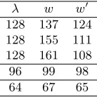
Unlike the list wlist, which is secret, we can choose w0 in a way that the list wlist0 is not secret (provided thatb remains confidential). This can be achieved if w0_w+w> 22λ. Such a selection is shown in Table 2, for λ= 128. With this approach, a secure implementation needs to protect only operations that involve b, which is hopefully efficient because |b| << r. Indeed, this allows us to keep only the compact representation ofh0_0↓in memory, and perform (in Alg. 8) only |b|iterations. This costs |b| ×r memory accesses (to bytes), instead ofr×r as with the alternative.

λ w w0

128 137 124 128 155 111 128 161 108

96 99 98

64 67 65

Table 2: Examples forw0 such that w0_w+w >22λ_.

Remark 2. Our method needs to make a uniform random selection from the set of size w0_w+w

, of allw+w0 indices (positions between 0 andr−1) from which whichw0positions are labeled as ”fake”. In practice, we use Alg. 3 to choose (in constant time) the positions of the w+w0 bits. Subsequently, we use Alg. 3 to determine thew0 positions (inb) that are labeled as ”fake”.

Algorithm 8 U=CountUPCConstantTime(˜s,wlist, b)

Input:˜s- a redundant representation ofrbits syndromes,wlist0 - aw0 elements of the compact representation ofh00↓.ba flags list of lengthw+w0.

Output:U an array ofrbytes.

1: procedureCountUPCConstantTime(˜s,wlist0,b)

2: U=0

3: fori = 0, . . . , r−1do 4: forj = 0, . . . , w0−1do

5: U[i] = U[i] + (rotl(˜s,wlist0[j])[i] &b[wlist0[j]]) 6: returnU

Step III. (Recalculate the syndrome) in constant time. The straightforward im-plementation recalculates the syndrome (in a (n0r, r)-code) by means ofn0 poly-nomial multiplications (modulo xr_{+ 1) plusn}

add all the columns while masking out the ”unnecessary” ones, to execute in con-stant time. We point out that applying the fake bits technique toe, introduces additional overheads that, by our experiments, make it non competitive.

4

Results

This section provides the performance results of our study. For this study, we wrote new optimized code for all the algorithms discussed above.

The core functionality was written in x86 assembly, and wrapped by assisting C code. The implementations use thePCLMULQDQ,AES−NIand the AVX2 and AVX512 architecture extensions. The code was compiled with gcc (version 5.4.0) in 64-bit mode, using the ”O3” Optimization level, and run on a Linux (Ubuntu 16.04.3 LTS) OS.

The experiments were carried out on a platform equipped with the latest 8th Generation IntelR _CoreYT M _{processor (”Kaby Lake”) - Intel}R _XeonR Plat-inum 8124M CPU at 3.00 GHz CoreR _{i5−750. The platform has 70 GB RAM,} 32K L1d and L1i cache, 1,024K L2 cache, and 25,344K L3 cache. It was con-figured to disable the IntelR _{Turbo Boost Technology, and the Enhanced Intel} SpeedstepR _Technology.

The performance is reported in processor cycles counts or in cycles per byte (C/B), where lower is better, reflecting the performance per a single core. The results were obtained with the same measurement methodology, as follows. Each measured function was isolated, run 25 times (warm-up), followed by 100 itera-tions that were clocked (using the RDTSC instruction) and averaged. To mini-mize the effect of background tasks running on the system, each such experiment was repeated 10 times, and the minimum result was recorded.

Estimating the DFR To estimate the DFR, we generated (ephemeral) CAKE keys, encrypted a pseudorandom message, and rand the decoder code. This was done for the three values of interest r = 215_−49,215_−19,215_{+ 3. For each} r, the experiments were repeatedN times, and recorded the number (nf ail) of decoding failures. Aiming for 95% confidence interval, our estimated DFR upper bound is 3/Nwhennf ail/N = 0, andχ2

2nf ail,0.025/(2N) when 0< nf ail/N <20.

Detailed explanations are given in Appendix D.

Obviously, the DFR depends on the actual decoding algorithm. We used here the decoding algorithm of [34], and also a version optimized by incorporating the Reduced Weight optimization. The results are summarized in Table 3. The DFR upper bounds are roughly the same (around 10−7), with both decoders, for the close r values. This implies that, given the specific decoder(s), it is reasonable to prefer the value ofrwhich also leads to the best decoding performance. This aspect is discussed below.

Efficient hashing Fig. 3 compares OpenSSL’s [2] performance for serial SHA384 (and SHA256), to ourParallelizedHashSHA384

111,8 (andParallelizedHashSHA25655,16 ), for dif-ferent message lengths. It includes results from both AVX2 and AVX512 versions for the algorithms. The choices= 8 yields the bestParallelizedHashSHA384

Decoder r nf ail DFR bound (N = 108)

[34]

32,719 0 3×10−8 32,749 1 3.369×10−8 32,771 2 5.57×10−8

[34] with

Reduced Weight optimization

32,719 7 1.3×10−7 32,749 4 8.76×10−8 32,771 2 5.57×10−8

Table 3: DFR estimations (95% confidence interval) for r = 215_−49,215₋ 19,215_{+ 3. The first three rows result from implementing the decoder of [34].} The last three rows result from the same decoder, combined with the Reduced Weight optimization.

and a zmmregister can accommodate 8 lanes, the full capabilities of AVX512 can be realized withs= 8. Similarly,s= 16 yields the best AVX2 performance forParallelizedHashSHA256

55,16 . The graphs show that parallelizing SHA384 (SHA256) contributes significant speedups for sufficiently long messages, e. g., 3.5xfor a 8KB message (with SHA384). In our context, withr≈215_{, the QC-MDPC} pro-tocols indeed hash messages of such lengths (or more), and the savings can be of∼20,000 cycles.

AES-CTR-PRF Alg. 1 usesAES256. An optimizedAES256code, that pipelines AES−NIinstructions efficiently, can produce output at 0.91 C/B. Thus, the task of generating roughly 4KB of pseudorandom data (for the relevant r values in our context) consumes approximately≈3,700 cycles. This is much faster than invoking the RDRAND instruction, as proposed in [30], as this instruction has guarantee throughput of 200 cycles [27]. It is also faster than hashing, repeatedly, a 256-bit seed concatenated with a (short) counter (even if this computation is parallelized).

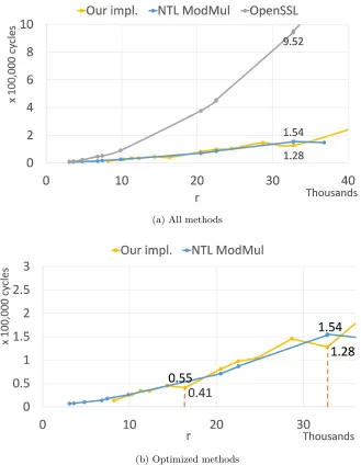
Polynomial multiplication Fig. 4 shows the performance results of our op-timized polynomial multiplication (modulo xr+ 1), compared to OpenSSL [2] (latest development version), and to NTL [38] (latest version) compiled with the GF2X library [37]. Panel (a) shows all the tested implementations and Panel (b) zooms into the two fastest ones.

(a) SHA256

(b) SHA384

Fig. 3: The performance (in C/B) of OpenSSL’s [2] serial hashing com-pared to ParallelizedHash AVX512 and AVX2 implementations. Top panel: serial SHA256 vs. ParallelizedHashSHA256_55,16 . Bottom panel: serial SHA384 vs. ParallelizedHashSHA384

111,8 .

Finally, we comment the following. We tested our optimized multiplications forr= 2α_{(2p+ 1)×64 and 2p+ 1≤11. These use recursive Karatsuba up to the} point where the degree of the polynomials is (2p+ 1)×64−1, and then switch to the schoolbook multiplication (see Section 3.5). We tried both horizontal and vertical methods. The horizontal schoolbook is faster in all cases, except for the casep= 0. Here, we found that the vertical schoolbook is faster for polynomials of degree 4×64−1.

Decoding The two time consuming steps of the BitFlip algorithm are ”Cal-culate the unsatisfied bits” and ”Recal”Cal-culate the syndrome”. Table 4 shows the performance of our AVX2 and AVX512 implementations of the first one. For each of these two architectures, we wrote an optimized code (CountUPC) and an optimized constant time implementation (CountUPCConstantTime). Two conclusion can be deduced: 1) AVX512 implementations are consistently∼1.5x faster than the AVX2 implementations; 2) The added overheads of incorporating side channel protection are 100−120% (AVX2) and 76−98% (AVX512), and increase withr.

Table 4 also shows that close values ofrmay lead to different performance. Consider the case where r1 = 211_{×p1, and r2 = 2}11_{×p2, where p1 <2}11 _< p2<212_{. The AVX512 implementation withr1performs better than withr2. A} similar phenomenon occurs with the AVX2 implementations, forr1= 29_{×p1, and} r2= 29_{×p2, andp1<2}9_{< p2<2}10_{. For example, the AVX512 implementation} withr1 = 22,511, is 1.09x faster than withr2= 22,531 (q= 43, p1= 211₋₁₇ andp2= 211+ 3).

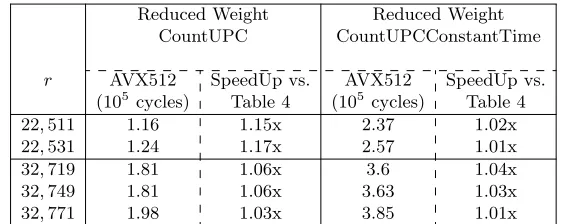
Section 3.6 proposed the Reduced Weight heuristic optimization. The results of this optimization, for an AVX512 implementation, are reported in Table 5, showing both CountUPC and CountUPCConstantTime with Reduced Weigh-tapplied. We choose α = 5 as a good balance point between performance and DFR.

CountUPC CountUPCConstantTime

r AVX2 AVX512 AVX2 AVX512

(105_{cycles) (10}5_{cycles) (10}5_{cycles) (10}5_cycles)

20,483 2.04 1.38 3.53 2.42

22,511 2.12 1.33 3.76 2.4

22,531 2.18 1.45 3.86 2.61

32,719 2.98 1.91 5.88 3.75

32,749 2.98 1.91 5.88 3.75

32,771 3.04 2.03 5.91 3.91

36,821 3.48 2.32 6.92 4.6

(a) All methods

(b) Optimized methods

Reduced Weight Reduced Weight CountUPC CountUPCConstantTime

r AVX512 SpeedUp vs. AVX512 SpeedUp vs. (105 _{cycles) Table 4 (10}5_{cycles) Table 4} 22,511 1.16 1.15x 2.37 1.02x 22,531 1.24 1.17x 2.57 1.01x

32,719 1.81 1.06x 3.6 1.04x

32,749 1.81 1.06x 3.63 1.03x 32,771 1.98 1.03x 3.85 1.01x

Table 5: Cycles comparison of CountUPC and CountUPCConstantTime imple-mented with the Reduced Weight optimization measured for different rvalues. We compare it to the ”normal” implementation in AVX512 (reported in Table 4) for calculating the speedup.

A somewhat surprising result was obtained for step III (Recalculate the syn-drome). The AVX2 optimized non-constant time implementation turned out to be slightly faster than the optimized AVX512 implementation. This happens because this step involved many memory accesses. To estimate the latency of step III, note that the performance of both implementations is proportional to the number of the corrected error bits. For example, with r=32,719, correcting 100 error bits consumes ∼270×100 = 27,000 cycles, which is almost 10x less than the latency of the matching constant time implementation. For constant time implementation of step III, our experiments showed that the fastest method is simply a direct calculating. For example, in CAKE (with r = 32,719), step III requires two polynomial multiplications and two additions. These consume roughly 2×120,000 = 240,000 cycles for the multiplication plus some (small) overhead for the two additions.

5

Conclusion

This paper offers a toolbox of primitives that can be leveraged towards ef-ficient and constant time implementations of QC-MDPC cryptosystems. The comparison of our implementations to alternative open source libraries (NTL and OpenSSL), indicates the functionalities that are improved. For example, our polynomial multiplication for degrees 214−1 and 215−1 is 1.34x and 1.2x faster than that of NTL, respectively, and our ParallelizedHashSHA384

8,111 is almost 3x faster than that of SHA384 in OpenSSL for large enough sizes.

We point out that the implementation described in [30] can also enjoy AVX512 capabilities, by using the instruction VPOPCNTQfor counting the upci (instead of usingPOPCNT).

As we notice, a proper choice of parameters can contribute to the resulting performance. Here are a few examples. With r = 32,719 = 215−49 optimal memory alignment led to a fast polynomial multiplication and decoding.

To achieve 128-bit quantum pre-image resistance, it is possible to use one of SHA512, SHA384, SHA256, or their parallelized variant, and the optimal choice depends on the length of the hashed buffer. Computing ParallelizedHash384

111,8 is faster than computingParallelizedHash512

111,8(due to the length of the final hash). Furthermore, a sparse buffer (e. g., in the last step of CAKE) can be compressed prior to hashing, in order to optimize the performance. Of course, in such cases, the cost of compression (which can be significant, especially if it needs to be carried out in constant time) needs to be weighed against the potential reduction in the hashing time.

The paper discusses optimization techniques for different building blocks of generic decoding algorithms. Our results can be used for enhancing the perfor-mance of a class of decoding algorithms. Given an algorithm, it is possible to predict the performance results by analyzing the cost of one decoding iteration, and multiplying it by the maximum number of iterations, that the algorithm defines. We provide one example.

Example 10. Consider the caser= 32,719 = 215_{−49 andw= 137. A decoding} iteration consists of the above three steps, and the performance cost of each iteration is the corresponding sum. We provide the performance of each step, for a constant time implementation (the numbers in parentheses correspond to non-constant time implementations), based on our results: ”CountUPC” performs at 375,000 (191,000) cycles, ”Find and compare the threshold” at 375,000 (20,000) cycles, and ”Recalculate the syndrome” at 250,000 (∼27,000) cycles. The sum is 1,000,000 (238,000) cycles per iteration.

In this example, we use the decoder of [34] and a constant time implementa-tion. Note that the performance of such implementation depends on themaximal

number of iterations, whereas a non-constant time implementation depends on theaveragenumber of iterations. To estimate the maximum / average number of iterations (withr= 32719), we setδ= 6 and ran it on 2×106 _{encoded random} inputs. The observed maximum and average number of iteration was 20 and 8, respectively. We can therefore estimate that constant-time decoding with this al-gorithm, choice of parameters, and 20 iterations which leads toDF R∼1.5×10−6 would perform at ∼20,000,000 cycles (8×238,000 = 1,904,000 cycles with a non-constant time implementation), on the ”Kaby Lake” platform. Our actual measurements agree with this estimation.

when run on an AVX2 platform 3_{. Our∼9x speedup is due to the optimized} primitives that leverage the capabilities of the AVX512 features.

Our choice of 20 iterations is a property of the algorithm in [34], and our the experiments. However, other decoding algorithms can optimize for a reduced maximum number of iteration, and achieve better constant time performance. One example is the result in [11] that reports an optimization of (9,602,4, 801)-codes with w = 90, where DFR of 0.150 ×10−6 _{is achieved with maximum} number of iterations set to 7. A different trade off between performance and DFR is proposed by our Reduced Weightoptimization (see Table 3)).

Acknowledgments

This research was supported by the PQCRYPTO project, which was partially funded by the European Commission Horizon 2020 research Programme, grant #645622, by the Israel Science Foundation (grant No. 1018/16), by the BIU Center for Research in Applied Cryptography and Cyber Security, in conjunction with the Israel National Cyber Bureau in the Prime Minister’s Office, and by the Center for Cyber Law and Policy at the University of Haifa.

Opinions, findings, conclusions, and recommendations, expressed in this ma-terial, are those of the author(s), and do not necessarily reflect the views of their employers and the granting agencies.

References

1. −: Nist:post-quantum cryptography - call for proposals (September 2017),https:

//csrc.nist.gov/Projects/Post-Quantum-Cryptography

2. −: OpenSSL, Commit: 2dbfa8444bdf7669a54006c4a83d1e60ba374528. https://

github.com/openssl/openssl(Sep 2017)

3. Aguilar, C., Blazy, O., Deneuville, J.C., Gaborit, P., Z´emor, G.: Efficient encryption from random quasi-cyclic codes. arXiv preprint arXiv:1612.05572 (2016)

4. Baldi, M., Chiaraluce, F., Garello, R., Mininni, F.: Quasi-cyclic low-density parity-check codes in the McEliece cryptosystem. In: 2007 IEEE International Conference on Communications. pp. 951–956 (June 2007)

5. Baldi, M., Bianchi, M., Chiaraluce, F., Rosenthal, J., Schipani, D.: Using LDGM Codes and Sparse Syndromes to Achieve Digital Signatures, pp. 1–15. Springer Berlin Heidelberg, Berlin, Heidelberg (2013), https://doi.org/10. 1007/978-3-642-38616-9 1

6. Baldi, M., Bodrato, M., Chiaraluce, F.: A new analysis of the McEliece cryp-tosystem based on QC-LDPC codes. Security and Cryptography for Networks pp. 246–262 (2008)

7. Baldi, M., Chiaraluce, F., Garello, R.: On the usage of quasi-cyclic low-density parity-check codes in the McEliece cryptosystem. In: 2006 First International Con-ference on Communications and Electronics. pp. 305–310 (Oct 2006)

3 IntelR

Core 4770M CPU at 3.40 GHz CoreR

8. Barker, E.B., Kelsey, J.M.: SP 800-90A. recommendation for random number gen-eration using deterministic random bit generators. Tech. rep., Gaithersburg, MD, United States (2012)

9. Barreto, P.S.L.M., Gueron, S., Gueneysu, T., Misoczki, R., Persichetti, E., Sendrier, N., Tillich, J.P.: CAKE: Code-based Algorithm for Key Encapsulation. Cryptology ePrint Archive, Report 2017/757 (2017), http://eprint.iacr.org/ 2017/757

10. Cayrel, P.L., Hoffmann, G., Persichetti, E.: Efficient Implementation of a CCA2-Secure Variant of McEliece Using Generalized Srivastava Codes, pp. 138–155. Springer Berlin Heidelberg, Berlin, Heidelberg (2012),https://doi.org/10.1007/ 978-3-642-30057-8 9

11. Chaulet, J., Sendrier, N.: Worst case QC-MDPC decoder for McEliece cryptosys-tem. In: 2016 IEEE International Symposium on Information Theory (ISIT). pp. 1366–1370 (July 2016)

12. Courtois, N.T., Finiasz, M., Sendrier, N.: How to achieve a mceliece-based digital signature scheme. In: International Conference on the Theory and Application of Cryptology and Information Security. pp. 157–174. Springer (2001)

13. Deneuville, J.C., Gaborit, P., Z´emor, G.: Ouroboros: A Simple, Secure and Efficient Key Exchange Protocol Based on Coding Theory, pp. 18–34. Springer International Publishing, Cham (2017),https://doi.org/10.1007/978-3-319-59879-6 2

14. Faug`ere, J.C., Otmani, A., Perret, L., de Portzamparc, F., Tillich, J.P.: Structural cryptanalysis of McEliece schemes with compact keys. Designs, Codes and Cryp-tography 79(1), 87–112 (Apr 2016),https://doi.org/10. 1007/s10623-015-0036-z

15. Gallager, R.: Low-density parity-check codes. IRE Transactions on Information Theory 8(1), 21–28 (January 1962)

16. Gueron, S.: Intel’s new AES instructions for enhanced performance and security. In: FSE. vol. 5665, pp. 51–66. Springer (2009)

17. Gueron, S.: IntelR advanced encryption standard (AES) new instructions set Rev. 3.01. Intel Software Network (2010)

18. Gueron, S.: A j-lanes tree hashing mode and j-lanes SHA-256. Journal of Informa-tion Security 4(01), 7 (2013)

19. Gueron, S.: Parallelized hashing via j-lanes and j-pointers tree modes, with appli-cations to SHA-256. Journal of Information Security 5(03), 91 (2014)

20. Gueron, S., Kounavis, M.: Efficient implementation of the galois counter mode using a carry-less multiplier and a fast reduction algorithm. Information Process-ing Letters 110(14), 549 – 553 (2010), http://www.sciencedirect.com/science/ article/pii/S002001901000092X

21. Gueron, S., Kounavis, M.E.: IntelR carry-less multiplication instruction and its usage for computing the gcm mode. White Paper (2010)

22. Gueron, S., Krasnov, V.: Simultaneous hashing of multiple messages. Journal of Information Security 3(04), 319 (2012)

23. Gueron, S., Schlieker, F.: Speeding up R-LWE Post-quantum Key Exchange, pp. 187–198. Springer International Publishing, Cham (2016),https://doi.org/

10.1007/978-3-319-47560-8 12

24. Guo, Q., Johansson, T., Stankovski, P.: A Key Recovery Attack on MDPC with CCA Security Using Decoding Errors, pp. 789–815. Springer Berlin Heidelberg, Berlin, Heidelberg (2016),https://doi.org/10.1007/978-3-662-53887-6 29

26. Intel Corporation: Intel architecture instruction set extensions programming reference. https://software.intel.com/sites/default/files/managed/c5/15/

architecture-instruction-set-extensions-programming-reference.pdf

(Oc-tober 2017)

27. Intel Corporation: Intel intrinsic guide. https://software.intel.com/sites/

landingpage/IntrinsicsGuide/#text=rdrand&expand=4247(October 2017)

28. Jovanovic, B.D., Levy, P.S.: A look at the rule of three. The American Statistician 51(2), 137–139 (1997),http://www.jstor.org/stable/2685405

29. Kabatianskii, G., Krouk, E., Smeets, B.: A digital signature scheme based on ran-dom error-correcting codes, pp. 161–167. Springer Berlin Heidelberg, Berlin, Hei-delberg (1997),https://doi.org/10.1007/BFb0024461

30. Maurich, I.V., Oder, T., G¨uneysu, T.: Implementing QC-MDPC McEliece en-cryption. ACM Trans. Embed. Comput. Syst. 14(3), 44:1–44:27 (Apr 2015),

http://doi.acm.org/10.1145/2700102

31. McEliece, R.: A public-key cryptosystem based on algebraic. Coding Thv 4244, 114–116 (1978)

32. Misoczki, R., Barreto, P.S.L.M.: Compact McEliece Keys from Goppa Codes, pp. 376–392. Springer Berlin Heidelberg, Berlin, Heidelberg (2009),https://doi.org/

10.1007/978-3-642-05445-7 24

33. Misoczki, R., Tillich, J.P., Sendrier, N., Barreto, P.S.L.M.: MDPC-McEliece: New McEliece variants from moderate density parity-check codes. Cryptology ePrint Archive, Report 2012/409 (2012),http://eprint.iacr.org/2012/409

34. Misoczki, R., Tillich, J.P., Sendrier, N., Barreto, P.S.: MDPC-McEliece: New McEliece variants from moderate density parity-check codes. In: 2013 IEEE In-ternational Symposium on Information Theory. pp. 2069–2073 (July 2013) 35. Monico, C., Rosenthal, J., Shokrollahi, A.: Using low density parity check codes in

the McEliece cryptosystem. In: 2000 IEEE International Symposium on Informa-tion Theory (Cat. No.00CH37060). pp. 215–. IEEE (2000)

36. Phesso, A., Tillich, J.P.: An Efficient Attack on a Code-Based Signature Scheme, pp. 86–103. Springer International Publishing, Cham (2016), https://doi.org/

10.1007/978-3-319-29360-8 7

37. Pierrick Gaudry, Richard Brent, P.Z., Thome, E.: gf2x-1.2. https://

gforge.inria.fr/projects/gf2x/(July 2017)

38. Shoup, V.: Number theory c++ library (ntl) version 10.5.0.http://www.shoup.net/ ntl(July 2017)

39. Stern, J.: A new identification scheme based on syndrome decoding. In: Annual International Cryptology Conference. pp. 13–21. Springer (1993)

A

AES-CTR-PRF

Algorithm 9 s=AES-CTR-PRF-Init(seed,maxInvokation)

Input:seed(32 bytes),maxInvokation(4 bytes) Output:s(AES-CTR-PRF state)

1: procedureAES-CTR-PRF-Init(seed,maxInvokation) 2: s.seed=seed

3: s.pos= 16

4: s.buffer=N U LL

5: s.=encode128(0)

6: s.remInvokations=maxInvokation

7: returns

Algorithm 10 A=AES-CTR-PRF(s, len)

Input:s(AES-CTR-PRFstate),len

Output:A(lenbytes), the updated AES-CTR-PRFstates

Exception:SeedOverUseError(seed overused). 1: procedure_{tmp=PerformAES}(s)

2: if s.remInvokations= 0then

3: raiseSeedOverUseErrorexception 4: tmp[15 : 0] =AES256s.seed(encode128(s.j)) 5: s.j=s.j+ 1

6: s.remInvokations=s.remInvokations−1 7: returntmp

8: procedure_AES-CTR-PRF(s,NB)

9: if len+s.pos<= 16then .Buffer has enough data. 10: A[len−1 : 0] =s.buffer[s.pos+len−1 :s.pos]

11: s.pos=s.pos+len

12: else

13: idx = 16−s.pos .calculate the buffer content length. 14: if idx>0then

15: A[idx−1 : 0] =s.buffer[15 :s.pos] 16: s.pos= 0

17: whilelen−idx >= 16do .Copy fullAES256blocks 18: A[idx + 15 : idx] = PerformAES(s)

19: idx = idx + 16

20: s.buffer= PerformAES(s) .Handle the tail.

21: s.pos=len−idx

22: A[len−1 : idx] =s.buffer[s.pos−1 : 0] 23: returnA[len−1 : 0],s

B

GenPseudoRand example

I n p u t s :

len = 141

s . s e e d = 0 0 0 0 0 0 0 0 0 0 0 0 0 0 0 0 0 0 0 0 0 0 0 0 0 0 0 0 0 0 0 0 0 0 0 0 0 0 0 0 0 0 0 0 0 0 0 0 0 0 0 0 0 0 0 0 0 0 0 0 0 0 0 0 s . j = 1

s . pos = 0

C T R 0 = e n c o d e 1 2 8 (0)

= 0 0 0 0 0 0 0 0 0 0 0 0 0 0 0 0 0 0 0 0 0 0 0 0 0 0 0 0 0 0 0 0 s . b u f f e r = A E S 2 5 6 ( s . seed , C T R 0 )

= 8 7 2 0 8 4 9 2 1 4 a 2 4 8 a d 8 9 8 9 4 0 a 2 7 8 c 0 9 5 d c

AES - C T R _ P R F i n t e r n a l v a l u e s :

A[ 1 5 : 0 ] = 8 7 2 0 8 4 9 2 1 4 a 2 4 8 a d 8 9 8 9 4 0 a 2 7 8 c 0 9 5 d c C T R 1 = e n c o d e 1 2 8 (1)

= 0 0 0 0 0 0 0 0 0 0 0 0 0 0 0 0 0 0 0 0 0 0 0 0 0 0 0 0 0 0 0 1 s . b u f f e r = A E S 2 5 6 ( s . seed , C T R 1 )

= d 3 3 c a 5 b f 3 e 1 3 9 3 4 5 6 8 b 8 4 f 6 b d 8 f 3 7 5 5 2 s . j = 2

s . pos = 2 A[ 1 7 : 1 6 ] = 7 5 5 2

O u t p u t s :

A[ 1 7 : 0 ] = 1 5 5 2 8 7 2 0 8 4 9 2 1 4 a 2 4 8 a d 8 9 8 9 4 0 a 2 7 8 c 0 9 5 d c

C

ParallelizedHash

8,111

example

ParallelizedHashSHA384

8,111 of the array of la = 2,000 byte array[j] = j (mod 255), j= 0, . . . ,la−1.

la = 2,000 ls = 239 lrem = 88

cdcccbcac9c8c7c6c5c4c3c2c1c0bfbebdbcbbbab9b8b7b6 b5b4b3b2b1b0afaeadacabaaa9a8a7a6a5a4a3a2a1a09f9e 9d9c9b9a999897969594939291908f8e8d8c8b8a89888786 8584838281807f7e7d7c7b7a797877767574737271706f6e 6d6c6b6a696867666564636261605f5e5d5c5b5a59585756 5554535251504f4e4d4c4b4a494847464544434241403f3e 3d3c3b3a393837363534333231302f2e2d2c2b2a29282726 2524232221201f1e1d1c1b1a191817161514131211100f0e 0d0c0b0a09080706050403020100fefdfcfbfaf9f8f7f6f5 ...

5f5e5d5c5b5a595857565554535251504f4e4d4c4b4a4948 47464544434241403f3e3d3c3b3a39383736353433323130 2f2e2d2c2b2a292827262524232221201f1e1d1c1b1a1918 17161514131211100f0e0d0c0b0a09080706050403020100

X[0 = 736aed26a8c4ed0add98f587bcaf349f2b748029eeaf3715 769f162d8343445c63ee3c4a0f606dbb498c787a07cf5625

X[1] = a24f959fd7b64bf4428ca7947133d1ceb2278f12ab37ee6c 29298ba72d48d33d3efd3490d84d22b227f78a1454c055a9

X[2] = 9c6f1f05fd0069788e5e555e1dd1648f61d222728d7c7357 3c4859b2b84b5d443737a883f9afdfbca5d9bc6bd1bd5f95

X[3] = 6ea3e8fd041d49db9b96fa39426637d3493dc889e2d5bd86 faff2ca73e93e57669eccfa46088561529fd3d91d709a240

X[4] = 4e2335af0345f0f6823cd4b569dcfa4b84515919c6afc150 844b904b96b64578ad9c375058d5c5f2d0980ccc021e00f6

X[5] = 0a8736a0be9cc12199207c4ef2df31e12ba32e47fd2ef356 7ca8230694b0c09c93bb5b029fe51475223f021c201f8b28

X[6] = 192f5227698c87d8e6d2f704c501757a902629263e57ead6 958d99aaceccd301019214d0cc6371d9036e76a8b832b5a1

X[7] = 09d013edf0a6f784c6e3b049069788a91030a9fc39de03db 6a748ca48f723614ef82533f3ead5b63764b18a5a29a1488

Y = d6d5d4d3d2d1d0cfcecdcccbcac9c8c7c6c5c4c3c2c1c0bf bebdbcbbbab9b8b7b6b5b4b3b2b1b0afaeadacabaaa9a8a7 a6a5a4a3a2a1a09f9e9d9c9b9a999897969594939291908f 8e8d8c8b8a898887868584838281807f

bebdbcbbbab9b8b7b6b5b4b3b2b1b0afaeadacabaaa9a8a7 a6a5a4a3a2a1a09f9e9d9c9b9a999897969594939291908f 8e8d8c8b8a898887868584838281807f09d013edf0a6f784 c6e3b049069788a91030a9fc39de03db6a748ca48f723614 ef82533f3ead5b63764b18a5a29a1488192f5227698c87d8 e6d2f704c501757a902629263e57ead6958d99aaceccd301 019214d0cc6371d9036e76a8b832b5a10a8736a0be9cc121 99207c4ef2df31e12ba32e47fd2ef3567ca8230694b0c09c 93bb5b029fe51475223f021c201f8b284e2335af0345f0f6 823cd4b569dcfa4b84515919c6afc150844b904b96b64578 ad9c375058d5c5f2d0980ccc021e00f66ea3e8fd041d49db 9b96fa39426637d3493dc889e2d5bd86faff2ca73e93e576 69eccfa46088561529fd3d91d709a2409c6f1f05fd006978 8e5e555e1dd1648f61d222728d7c73573c4859b2b84b5d44 3737a883f9afdfbca5d9bc6bd1bd5f95a24f959fd7b64bf4 428ca7947133d1ceb2278f12ab37ee6c29298ba72d48d33d 3efd3490d84d22b227f78a1454c055a9736aed26a8c4ed0a dd98f587bcaf349f2b748029eeaf3715769f162d8343445c 63ee3c4a0f606dbb498c787a07cf5625

digest = 449d8e98c4805b8e551d7520466a3ebdebb5d3230009486a 1687da888616305ca6fa1d9c5d890835f512e535e651cbcb

D

Estimating the DFR

To estimate the DFR from N experiments that show nf ail decoding failures, with a 95% confidence interval, we use the following methodology.

If nf ail = 0, we use the ”Rule of Three” [28] that places the DFR in the interval [0,3/N], which implies the upper bound DFR ≤ 3/N. Let ˆp =

nf ail

N denote the maximum-likelihood estimator for the DFR, and let X ∼ Bin(N,DFR) denote the distribution of the failures. This is well approximated by the Poisson distribution X ∼ P oiss(N×DFR), for sufficiently large N. If ˆ

p < 20, we use the χ2 _{distribution as an approximation of the related} Pois-son distribution X ∼ P oiss(N×DFR), getting the confidence interval 1

2N × [χ2

2(nf ail+1),1−α/2, χ

2

2nf ail,α/2]. Withα= 0.05, this gives the upper bound DFR≤

1 2N ×χ

2

2nf ail,0.025. In case ˆp≥20, the Poisson distribution can be approximated

by the Gaussian distribution, giving DFR≤pˆ+_Zα× p

ˆ