ISSN 2348 – 7968
Robust Tuning of Controller for SISO and MIMO Systems Using
Coefficient Diagram Method
Vasu PuligundlaP
1
P
and Jayanta PalP
2
P
1
P
Adama Science and Technology University, Ethiopia, P
2
P
Indian Institute of Technology, Kharagpur, India
Abstract – In this paper, robust tuning of controller for SISO and MIMO systems is considered. Firstly Power System Stabilizer(PSS) is taken as an example for SISO System. The first objective is to tune PID-PSS so that closed-loop response of a single machine connected to an infinite bus system (SMIB) is made stable over a wider range of operating points while maintaining the desired damping. The Coefficient Diagram Method (CDM) is used for choosing the coefficients of the target characteristic polynomial of the closed loop system based on performance criteria; such as equivalent time constant, stability indices and stability limits. Standard Manabe form is used for choosing the stability indices. The parametric uncertainties are handled by adding a pre-filter that increases the degree of the CDM based controller (PID-PSS) by one. Genetic Algorithm and pole coloring technique are then used for tuning the pre-filter by minimizing the shift in the closed-loop poles due to perturbations. The robustness of the designed feedback controller for SMIB is verified by using the Kharitonov Theorem and the Zero-exclusion condition. ; Secondly Controller designed for MIMO systems taking some examples which include stable and unstable systems. Pressurized flow-box, Four-input four-output gas fired furnace problem, Mueller’s two-shaft aircraft gas turbine are considered as an examples for MIMO Systems. The second objective is to tune a Diagonal controllers for these MIMO systems, such that each output can be controlled independent of other outputs, by varying particular input only. Standard Manabe form and CDM are used for choosing the coefficients of closed loop characteristic equation.
Index Terms-- Power System Stabilizers, Power system dynamic stability, Coefficient Diagram Method, Genetic Algorithm, Robust control, MIMO systems, Zero Frequency Decoupler.
I. INTRODUCTION
There has been considerable effort for solving the problem of low frequency oscillations leading to instability of power systems. These modes of oscillations are characterized by low mechanical natural frequencies in the range of 0.3-2.0 Hz. To damp out the oscillations, power system stabilizers (PSS) are used to inject a supplementary signal at the voltage reference input of the automatic voltage regulator (AVR). Conventionally a single-input single-output feedback
controller is used as PSS. As an input signal to a conventional PSS, anyone of the three signals i.e., machine shaft speed, ac bus frequency or accelerating power can be used. Most commonly used input signal is the machine shaft speed [10].
Many research papers have been published in this area [2, 8, 9]. The PSS design normally uses classical control theory and is based on a model of the power system linearized at some operating point. Properly tuned, a PSS can considerably enhance the dynamic performance of a power system.
Some work in the area of designing self-tuning, adaptive and robust PSS [2, 8] has been reported for achieving better control over wide range of load variations. However, the complexity and/or real-time computational requirement of such controller preclude their use in actual power plants.
Changes in transmission networks, generation and load patterns results in changes in operating conditions of power systems. Thus, the small signal dynamic behavior of a power system is varied, which can be expressed as a parametric uncertainty in the small signal linearized model of the system. In this work, we design a robust PSS so that adequate damping can be provided over a wide range of operating conditions. This work was motivated by some papers [2, 8, 9], where the quantitative feedback theory (QFT) [8], LMI technique [2] and Optimization Techniques [9] have been used for designing a robust PSS.
In this paper coefficient diagram method [3], an algebraic design approach (or polynomial method), is used. The time-domain performance of a system is closely related with its poles or characteristic polynomial. The characteristic polynomial can be defined from stability and response specification, but it is very difficult to choose it with guarantee of robustness. The CDM standard form [3] is used for choosing the target closed loop characteristic polynomial. Although the CDM results in pretty robust controllers, if there are large uncertainties in the system CDM itself may not be enough to satisfy robust stability and performance requirements. The CDM design method is extended to handle all possible parametric uncertainties with satisfactory performance by increasing the degree of the controller offered by the CDM by one. A pole-zero pair is introduced to create extra design freedoms and then a pole-coloring technique [4] to guarantee robust pole assignment. The pole-zero pair is tuned using Genetic Algorithm by minimizing the shift in the closed-loop poles due to perturbations.
II. METHOD A. Concept of CDM:
In CDM, the controllers are designed based on the stability index known as 𝛾𝑖 and the equivalent time constant known as τ which are synthesized from the characteristic polynomial of the closed-loop transfer function.
𝑃(𝑠) = ansn+⋯+ a1s + a0=�aisi n
i=0
− − − −(3)
From the characteristic polynomial P(s) given in eq. (3), the stability index 𝛾𝑖 and the equivalent time constant τ are respectively described in general term as the following equations [3]
𝛾𝑖= 𝑎1 2
𝑎𝑖+1𝑎𝑖−1,𝑖= 1~𝑛 −1 − − − −(4)
𝜏=𝑎𝑎1
0− − − −(5)
In order to meet the specifications, the equivalent time constant τ and the stability index 𝛾𝑖 are normally chosen as
𝜏=2.5 ~𝑡𝑠 𝑡3𝑠
𝛾𝑖> 1.5γi∗
Where ts is the specified settling time and γi∗ is the stability limit defined as
γi∗= 1
γi+1+ 1
γi−1,i= 1~n −1, γn=γ0=∞
In general the stability index is recommended as
𝛾𝑛−1~𝛾2= 2, 𝛾1= 2.5− − − −(6)
known as standard stability index.
Finally the characteristic polynomial known as the desired characteristic polynomial can be expressed as
𝑃(𝑠) =𝑎0���(� 1
𝛾𝑖−𝑗𝑗
𝑖−1
𝑗=1 𝑛
𝑖=2
�(𝜏𝑠)𝑖�+𝜏𝑠+ 1]
= ansn+⋯+ a1s + a0,
Where, an, an−1, … a0 are the coefficients of the desired characteristic polynomial.
B. Pole coloring [4]:
Consider the simple case of a third-order system where the nominal poles and perturbed poles for a fixed q (perturbations) are given in Fig1. Here, assume that big points represent perturbed poles and small points represent nominal poles corresponds to which of the perturbed poles is called ‘pole coloring’.
C. Graphical approach for checking robustness [5]:
Consider a real general polynomial p(s) of degree ‘n’ as given below:
𝑝(𝑠) =𝑎𝑛𝑠𝑛+𝑎𝑛−1𝑠𝑛−1+⋯+𝑎1𝑠+𝑎0− − − −(7)
The polynomial p(s) is said to be an interval polynomial if each coefficient is independent of the other and varies within an interval having a lower and upper bound [5]: i.e. 𝑎𝑖= [𝑎𝑖−,𝑎𝑖+],𝑖= 0,1,2, … ,𝑛. , such an uncertain polynomial is
said to have an independent uncertainty structure.
Kharitonov Theorem: The interval polynomial p(s) is robustly stable if and only if the following four Kharitonov polynomials:
𝐾1(𝑠) =𝑎0++𝑎1+𝑠+𝑎2−𝑠2+𝑎3−𝑠3+𝑎4+𝑠4+𝑎5+𝑠5+⋯
𝐾2(𝑠) =𝑎0−+𝑎1−𝑠+𝑎2+𝑠2+𝑎3+𝑠3+𝑎4−𝑠4+𝑎5−𝑠5+⋯
𝐾3(𝑠) =𝑎0−+𝑎1+𝑠+𝑎2+𝑠2+𝑎3−𝑠3+𝑎4−𝑠4+𝑎5+𝑠5+⋯
𝐾4(𝑠) =𝑎0++𝑎1−𝑠+𝑎2−𝑠2+𝑎3+𝑠3+𝑎4+𝑠4+𝑎5−𝑠5+⋯
− − − − −(8) are stable [5].
Given the interval polynomial p(s, a) as defined in eq. (7) and a fixed frequency ω=𝜔0, one can describe a set of possible values that 𝑝(𝑗ω0,𝑎) can assume as a varies over the box Q which can be shown as:
𝑝(𝑗𝜔0,𝑄) = { p(j𝜔0,𝑎) :a ϵ Q}
Then, p (j𝜔0,𝑄) can be termed as the Kharitonov rectangle [5] at frequency ω=𝜔0 with vertices which are obtained by evaluating the four Kharitonov polynomials, KRiR(s), i=1,2,3,4., as defined in eq. (8) , at s=j𝜔0. The rectangularity is proved in [5]. By varying the frequency from ω=0, and with ω increasing in discrete steps, results in the motion of the Kharitonov rectangle with the rectangle moving around the complex plane with vertices 𝐾𝑖(𝑗𝜔). The dimensions (size) of this rectangle vary with the frequency ω.
Zero Exclusion Condition: Suppose that an interval polynomial family p(s) has invariant degree and at least one stable member, the p(s) is robustly stable if and only if s=0 is excluded from the Kharitonov rectangle at all non-negative frequencies [5]; i.e. 0 ∉ p (jω, Q)
The zero exclusion condition suggests a simple graphical procedure for checking robust stability. By watching the motion of Kharitonov rectangle p (jω, Q) as ω varies from 0 to +∞, one can easily determine by inspection if the Zero
ISSN 2348 – 7968 Exclusion condition is satisfied. If it is satisfied, then one can
say that the polynomial family p(s) is robustly stable.
III. SISO SYSTEM (PSS)
By varying the operating conditions over a range which includes almost all practical operating conditions for the generator and by varying lengths of transmission lines includes very weak to very strong transmission systems, so the operating conditions are chosen in the intervals P[0.4 1.0], Q[-0.2 0.5] and X[Q[-0.2,0.7].
By taking a step difference of 0.1 in the values of P, Q and X, totally 336 combinations are obtained which corresponds to 336 operating points. Using the Heffron-Philips linearized model [6] of a single machine connected to an infinite bus (SMIB) system, 336 linearized models of the plant is constructed. The problem considered in [2], [8] is to design a feedback controller that maintains a damping ratio of at least 0.1 and real parts of all closed-loop poles less than -0.5 simultaneously for all operating points.
A. Power system model:
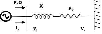
The Heffron-Philips linearized model [6] of a single machine connected to an infinite bus (SMIB) system is considered in this work. Fig.1 shows the line diagram of a synchronous machine connected to an infinite bus through a transmission line having resistance Re and reactance X
Fig.1. Line diagram of single machine connected to infinite bus.
The detailed derivation and assumptions are given in [7]. System data and state space representation are given in appendix.
B. PSS structure:
Case1: A simple PID-PSS is considered, when parameters are tuned using standard CDM only. The transfer function of PSS as:
𝐾(𝑠) =𝑘𝑑𝑠2+𝑠𝑘𝑝𝑠+𝑘𝑖− − − −(1)
Case2: A PID amended with a pole-zero pair is considered when CDM & pole-coloring are used. The transfer function of PSS as:
𝐾(𝑠) =�𝑠𝑠++𝑎𝑏� �𝑘𝑑𝑠2+𝑠𝑘𝑝𝑠+𝑘𝑖� − − − −(2)
The input to PSS is the machine shaft speed, ∆ω and the output is ∆U, i.e.
∆U= K(s) ∆ω
Fig. 2 Closed loop configuration of single-machine system.
The parameters of PSS viz. kRdR, kRpR, kRiR, a and b are tuned through combination of CDM, GA and pole-coloring techniques to meet the desired objectives.
IV. CONTROLLER DESIGN FOR SISO SYSTEM A family of 336 linearized models of the plants is constructed for grid of operating points as P,Q and 𝑋𝑒 vary independently in steps of 0.1 over the interval [0.4, 1.0], [-0.2, 0.5] and [0.2, 0.7] respectively. The reference terminal voltage is kept as ∆𝑉𝑅𝐸𝐹=0.05 and moment of inertia is calculated as M=2H. Open loop poles location: when P, Q, and Xeare varied independently in steps of 0.1 over the interval [0.4, 1.0], [-0.2, 0.5] and [0.2, 0.7] are shown in Fig.3.
Fig. 3 Open loop poles locations for all chosen perturbations
A. Designing a robust PID-PSS:
Step1: Let the light loading condition P=0.4, Q=-0.2 and X=Q=-0.2 be the nominal operating point, then corresponding transfer function will be
𝐺𝑙𝑖𝑔ℎ𝑡(𝑠) =𝑠4+ 21.1𝑠3+ 170.6−44.3𝑠2+ 1102.3𝑠 𝑠+ 4371
Step2:Choose controller to be designed as PID
Step3: Obtain the closed loop characteristic polynomial in terms of unknown controller parameters-
SMIB system
K(s)
+
+
∆ω ∆𝑉𝑅𝐸𝐹
∆U
P, Q
𝐈𝐚
X 𝐑𝐞
𝐕𝐭 𝐕∞
P(s) = s4+ 21.1s3+ (170.6𝑠2+ 44.3k d)s2
+�1102.3 + 44.3kp�s + (4371 + 44.3ki)
ai=[a5 a4a3a2a1a0]
=�1 21.1 (170.6𝑠2+ 44.3k
d) �1102.3
+ 44.3kp� (4371 + 44.3ki) � − − − −(9)
Step4: Choose the stability indices according to the CDM standard form Eq. (6)
As we have taken γi from standard form, stability conditions are satisfied, γ2>γ2∗
Or from R-H criterion a2>�a1
a3�a4+�
a3
a1�a0 is also satisfied.
Step5: From equations (4), (6) & (9), kRd R=1.1916, kRp R= 1.7636, kiRR= -42.3410.
The interval characteristic polynomial of the closed loop system becomes:
𝐺intervalI =[1,1]s4+[20.66, 21.13]s3+[229.22, 233.84]s2+
[708.82, 1974.81]s +[2726.75, 3686.83].
For this values of kRdR, kRp, Rand kiRR closed loop poles location, closed-loop system response to 5% disturbance step, and Kharitonov rectangles are shown in figures 4a, 4b and 4c respectively.
Fig.4a. Closed-loop poles location. Most dominant pole at -0.43, minimum damping ratio offered 5P
o
P
.
Fig.4b. Closed loop system response to a 5% disturbance step at all 336 operating points with kRd R= 1.1916, kRp R= 1.7636, kRiR =-42.3410.
Fig.4c. The Kharitonov Rectangles satisfying zero exclusion condition
The heavy loading condition, P=1.0, Q=0.5, X=0.7 be the nominal operating point
𝐺ℎ𝑒𝑎𝑣𝑦(𝑠) =𝑠4+ 20.66𝑠3+ 168.69−37.23𝑠2+ 569.62𝑠 𝑠+ 5798.4
Repeating steps 2 to 5, we finally obtain: kRd R=1.2020, kRpR=14.3134, kRiR=-94.5537.
By observing the pole locations in Fig.5, we can say that the controller designed with nominal operating condition as heavy loading condition is not robust. It was already mentioned that CDM does not always guarantee robustness. To get the flexibility in choosing any operating point as our nominal operating condition, we include a pre-filter (Eq. 2) and search for the unknown parameters a & b by using GA such that the stability indices (standard CDM) are [2 2 … 2.5].
Fig.5 closed-loop poles location shows that the controller is not robustly stable.
This will give the robustness if the pole-zero pair is properly tuned. Out of 336 operating points we can choose anyone as the nominal operating point for designing the controller and we can attain robustness by proper tuning of pre-filter.
B. Fitness calculation for GA:
1. Using the nominal transfer function (with no perturbations), for a particular value of a and b (supplied by GA) find the values of kRdR, kRpR & kRiR by using equations (4), (6) and characteristic polynomial. Find the roots of closed loop characteristic polynomial
ISSN 2348 – 7968 2. By making perturbation in P, Q and X obtain the open loop
transfer function from equations mentioned in appendix. Find the closed loop transfer function, with the same controller designed at nominal operating point, which gives perturbed pole locations.
3. Using the pole coloring technique, calculate the distance between the corresponding nominal poles and the perturbed poles let sum of the distances be dij (distance corresponding to ith pertubation and jth iteration)
4. Repeat the steps 2 & 3 for 336 times, add all dij′s, 𝐷𝑗=� 𝑑𝑖𝑗
336
𝑖=1 , (𝐷𝑗 𝑖𝑠 𝑡𝑜 𝑏𝑒 𝑚𝑖𝑛𝑖𝑚𝑖𝑠𝑒𝑑
).
C. Robust PSS (PID and a pre-filter):
Step1: Let the heavy loading condition P=1.0, Q=0.5, X=0.7, be the nominal operating point
𝐺ℎ𝑒𝑎𝑣𝑦(𝑠) =𝑠4+ 20.66𝑠3+ 168.69−37.23𝑠2+ 569.62𝑠 𝑠+ 5798.4
Step2: Choose controller to be designed as in Eq. (2) Step3: Obtain closed-loop Characteristic polynomial coefficients:
𝑎5= 1;
𝑎4= 20.66 +𝑏;
𝑎3= 20.66𝑏+ 168.69 + 37.23𝑘𝑑
𝑎2= 168.69𝑏+ 569.62 + 37.23𝑎𝑘𝑑+ 37.23𝑘𝑝
𝑎1= 569.62𝑏+ 5798.4 + 37.23𝑎𝑘𝑝+ 37.23𝑘𝑖
𝑎0= 5798.4𝑏+ 37.23𝑎𝑘𝑖
Step4: Choose the stability indices according to the standard CDM as in Eq. (6)
Step5: From equations (4), (6) and step3, we can get the values of kRdR, kRpR & kRiR, for every given values of a and b. Using GA tune a and b by minimizing DRjR.
kRdR =2.93, kRpR = 15.54, kRiR = -36.23, a = 9.51, b = 11.36. The interval characteristic polynomial of the closed loop
system becomes:
𝐺intervalI =[1, 1]s5+[32.02, 32.49]s4+[502.97, 605.57]s3+
[5123.73, 5645.31]s2+[19024.95, 31328.33]s +
[12350.93, 74198.11].
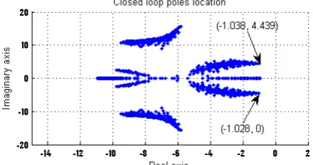
Fig.6a. Closed-loop poles location. Most dominant pole is at -1.028, minimum damping ratio offered is 13.16P
o
P
.
Fig.6b. Closed loop system response to a 5% disturbance step at all 336 operating points with kRd R= 2.93, kRp R= 15.54, kRiR = -36.23, a = 9.51, b= 11.36.
Fig.6c The Kharitonov Rectangles satisfying zero exclusion condition
In table-1 we can find robust PSS designed at different operating points (light, average, heavy and worst loading conditions) as our nominal operating condition, which are satisfying all the closed loop requirements as mentioned in the problem.
TABLE I
ROBUST PSS DESIGNED BY CHOOSING DIFFERENT OPERATING POINTS AS NOMINAL OPERATING CONDITIONS
Loading Condition:
[P,Q,X]
PSS [kd, kp, ki, a,b]
Most Dominan
t Pole
Min. Damping
Ratio (factor) Light:
[0.4, -0.2,0.2 ]
[3.58,20.75,-42.75,7.41,14.54] -0.77
9.67P
o
P
(0.17 ) Average:
[0.7,0.15,0.45 ]
[3.08,15.60,-61.17,7.66,14.66] -0.67
8.57P
o
P
(0.15)
Heavy: [1.0,0.5,0.7]
[2.93,15.54,-36.23,9.51,11.36] -1.03
13.16P
o
P
(0.23) Worst:
[1.0,0.0,0.7]
[3.18,6.33,-45.38,10.81,12.15
]
-0.71 9.61P
o
P
(0.17) In all the cases most dominant pole is always less than -0.5, and the minimum damping factor offered is always greater than 0.1. Thus the performance requirements are achieved.
V. CONTROLLER DESIGN FOR MIMO SYSTEMS A. Stable systems:
Unity negative feedback configuration using diagonal controller and ZFD:
Fig.7
ZFD is the inverse of the zero frequency (steady-state) gain matrix of the plant P(s), i.e. (P(0))P
-1
P
.
U
Example1:U [Ref.11] The open loop transfer function of a pressurized flow-box is considered in the example: Plant TFM:
P(s)
=�
0.0336 s + 0.395
1.03s
s2+ 0.395s + 1.26e −4
9.66e −4s + 0.117e −4 s2+ 0.395s + 1.26e −4
−0.0114 s2+ 0.395s + 1.26e −4
�
ZFD =�0.01206511.7560 −0.0110530 �
Choosing controller as diagonal PI controller: Cd(𝑠) =�
a𝑠+b
𝑠 0
0 c𝑠+𝑠 d �
By finding the closed loop transfer function of the system Fig7: we get the closed loop characteristic polynomial coefficients as,
a0= 2733*b*d;
a1= 2733*a*d+2733*b+0.8814e7*b*d+2508*d+2733*b*c; a2=-0.2240e9*b+2508*c+0.8108e7*d+2733*a*c+
0.8814e7*b*c+0.4287e8*b*d+2733*a+0.8814e7*a*d; a3=0 .4287e8*a*d+0.5205e8*b*d+0.8108e7*c+0.4287e8*b*c
+0.8814e7*a*c+0.7893e9*d-0.2240e9*a-0.7295e12*b;
a4=0.7893e9*c+0.3842e10*d+0.5205e8*b*c-0.3691e13*b+0.5205e8*a*d-0.7295e12*a +0.4287e8*a*c;
a5= -0.4672e13*b+0.3842e10*c+
0.5205e8*a*c-0.3691e13*a+0.4800e10*d; a6= 0.4800e10*c-0.4672e13*a;
By using equations (4) & (6)
[a,b,c,d] = 1.0e+005* [-2.420, -0.0567, -4.3036, -0.01161];
Fig.8
U
Example 2:U [Ref. 12]
In this example, we consider the four-input four-output gas fired furnace problem. The furnace has the following transfer function matrix.
P(s) =
⎣ ⎢ ⎢ ⎢ ⎢ ⎢ ⎢ ⎢
⎡4s + 11 5s + 10.7 5s + 10.3 5s + 10.2 0.6
5s + 1 1 4s + 1
0.4 5s + 1
0.35 5s + 1 0.35
5s + 1 0.4 5s + 1
1 4s + 1
0.6 5s + 1 0.2
5s + 1 0.3 5s + 1
0.7 5s + 1
1 4s + 1⎦⎥
⎥ ⎥ ⎥ ⎥ ⎥ ⎥ ⎤
ZFD =�
1.7484 −1.2112 −0.1586 0.1694 −0.9796 1.8745 −0.2307 −0.3217 −0.3217 −0.2307 1.8745 −0.9796 0.1694 −0.1586 −1.2112 1.7484
�
Choosing controller as diagonal PI controller: Diagonal
Controlle
MIMO Plant ZFD
y(s) r(s) -
+
ISSN 2348 – 7968 Cd(𝑠)
=
⎣ ⎢ ⎢ ⎢ ⎢ ⎢ ⎢ ⎢
⎡kp1∗ 𝑠𝑠+ki1 0 0 0
0 kp2∗ 𝑠𝑠+ki2 0 0
0 0 kp3∗ 𝑠𝑠+ki3 0
0 0 0 kp4∗ 𝑠𝑠+ki4⎦⎥
⎥ ⎥ ⎥ ⎥ ⎥ ⎥ ⎤
The closed loop characteristic polynomial coefficients: a5=.2500e5*kp4*kp2*kp3+.2500e5*kp1*kp4*kp2+.2500e5* kp1*kp2*kp3+.2500e5*kp1*kp4*kp3.
a4=4999.*kp1*kp4*kp2+.2500e5*kp1*ki4*kp3+5001.*kp1*k p2*kp3+.2500e5*kp1*kp4*ki2+.2500e5*kp4*ki2*kp3+.2500 e5*kp4*ki1*kp3+.2500e5*kp1*kp2*ki3+.2500e5*ki4*kp2*k p3+4999.*kp1*kp4*kp3+.2500e5*kp1*ki2*kp3+.2500e5*kp4 *kp2*ki3+.2500e5*ki1*kp2*kp3+.2500e5*kp4*kp2*ki1+.25 00e5*kp1*kp4*ki3+5002.*kp1*kp4*kp2*kp3+5001.*kp4*kp 2*kp3+.2500e5*kp1*ki4*kp2.
a3=.2500e5*ki4*kp2*ki3+.2500e5*ki4*ki2*kp3+5001.*ki4* kp2*kp3+5001.*kp4*ki2*kp3+5001.*kp4*kp2*ki3+.2500e5* kp4*ki2*ki1+4999.*kp1*ki4*kp3+.2500e5*kp1*ki4*ki2+499 9.*kp1*ki4*kp2+.2500e5*ki4*ki1*kp3+.2500e5*ki1*kp2*ki 3+.2500e5*ki1*ki2*kp3+.2500e5*kp4*ki1*ki3+4999.*kp4*k i1*kp3+5001.*ki1*kp2*kp3+4999.*kp1*kp4*ki2+.2500e5*ki 4*kp2*ki1+5001.*kp1*kp2*ki3+.2500e5*kp1*ki4*ki3+5001. *kp1*ki2*kp3+.2500e5*kp1*ki2*ki3+4999.*kp1*kp4*ki3+.2 500e5*kp4*ki2*ki3+5002.*kp1*kp4*kp2*ki3+5002.*kp1*kp 4*ki2*kp3+5002.*kp1*ki4*kp2*kp3+5002.*kp4*kp2*ki1*kp 3+4999.*kp4*kp2*ki1.
a2=5002.*kp1*kp4*ki2*ki3+5002.*kp4*kp2*ki1*ki3+.2500e 5*ki4*ki2*ki3+5002.*ki4*kp2*ki1*kp3+5001.*ki1*ki2*kp3 +5001.*ki1*kp2*ki3+5002.*kp1*ki4*ki2*kp3+5002.*kp1*ki 4*kp2*ki3+5001.*ki4*ki2*kp3+4999.*kp1*ki4*ki2+.2500e5 *ki2*ki1*ki4+5001.*kp1*ki2*ki3+4999.*kp1*ki4*ki3+4999. *kp4*ki2*ki1+4999.*ki4*kp2*ki1+5001.*kp4*ki2*ki3+4999. *kp4*ki1*ki3+.2500e5*ki4*ki1*ki3+5001.*ki4*kp2*ki3+499 9.*ki4*ki1*kp3+.2500e5*ki2*ki1*ki3+5002.*kp4*ki2*ki1*k p3.
a1=5002.*ki1*ki4*ki2*kp3+4999.*ki4*ki1*ki3+5002.*kp4*k i2*ki1*ki3+4999.*ki2*ki1*ki4+5001.*ki4*ki2*ki3+5002.*kp 1*ki4*ki2*ki3+5002.*ki4*kp2*ki1*ki3+5001.*ki2*ki1*ki3. a0=5002.*ki4*ki2*ki1*ki3
By using equations (2) & (4)
Cd(𝑠) =
⎣ ⎢ ⎢ ⎢ ⎢
⎡22.1s+4s .68 0 0 0
0 1.741s+1s .501 0 0
0 0 17.37s+3s .675 0
0 0 0 22.1s+4s .68⎦⎥ ⎥ ⎥ ⎥ ⎤
Fig.9
U
Example 3:U [Ref. 13]
The plant considered is Mueller’s two-shaft aircraft gas turbine.
Plant TFM: P(s)
=∆(s)1 �14.9685.2𝑠2𝑠2+ 8642.688+ 1521.432𝑠𝑠+ 12268.8 124000+ 2543.2 95150𝑠2𝑠2+ 1132094.7+ 1492588𝑠𝑠+ 2+ 1
∆(s) = s4+ 113.225s3+ 1357.275s2+ 3502.75s + 2525
ZFD =�−0.00200.4054 −0.28980.0004�
Cd(𝑠) =�
a𝑠+b
𝑠 0
0 c𝑠+d 𝑠
�
The closed loop characteristic polynomial coefficients: a8=.3322e5*a+1709.*c;
a7=1709.*d+.4112e7*a+.3322e5*b+.2137e6*c;
a6=.4643e7*c+.3166e5*c*a+.2137e6*d+.4112e7*b+.8491e8* a;
a5=.8491e8*b+.3585e7*c*a+.4643e7*d+.3166e5*c*b+.3166e 5*d*a+.3704e8*c+.5972e9*a;
a4=.4295e8*c*a+.3585e7*d*a+.3166e5*d*b+.3585e7*c*b+.5 972e9*b+.3704e8*d+.1360e10*a+.1181e9*c;
a3=.1617e9*c+.4295e8*c*b+.1107e9*c*a+.1004e10*a+.1360 e10*b+.3585e7*d*b+.4295e8*d*a+.1181e9*d;
a2=.8340e8*a+.1107e9*d*a+.1004e10*b+.1107e9*c*b+.796 9e8*c*a+.1617e9*d+.7969e8*c+.4295e8*d*b;
a1=.7969e8*d+.7969e8*c*b+.1107e9*d*b+.8340e8*b+.7969 e8*d*a;
a0=.7969e8*d*b;
By using equations (2) & (4) [a, b, c, d] = [0.8547, 1.4018, -0.004, 330.8]
Fig.10 B.Unstable systems:
Two-Loop Unity Negative Feedback Configuration: Fig.11
U
Example 4:U [Ref. 14]
The state space matrices of an unstable system are given by
A =�−2.37517.719 −0.8575.50 −1.0005.250
−14.766 −6.75 −7.375� ; B =�
0 0
1 0
−1 1�; C =�0 0.3 1.80 0 −4� ; D =�0 0
0 0� ;
The transfer function matrix is
1
s3+10.5𝑠2+4.5𝑠−5 �−1.5𝑠
2−14.7𝑠+ 3 1.8𝑠2+ 4.05𝑠+ 2.25
4𝑠2+ 39.5𝑠 −5 −4𝑠2−12.5𝑠 −8.5�
The poles are at: -1,-10 and +0.5.
Eigen value assignment by the method given in [224]. The desired characteristic polynomial is
(s+1)(s+10)(s+2)
The gain matrix for stabilization is obtained as K =�h1
h2� [f1 f2]=�
24.975 10.1 0 0 �.
The closed-loop TFM, Z(s) of the stabilized system is found to be
Z(s)
=d(s)1 �−1.5s4s2+ 39.5s2−14.7s + 3.0076 1.8s−5.0164 −4s22−+ 16.17s42.47s + 62.688−26.539� d(s) = s3+ 13.438s2+ 36.316s + 19.441
This stabilized closed-loop TFM (minor loop) will serve as the plant TFM in the next step, i.e. design of outer loop for performance.
ZFD =�21.9945 9.31141.76 1.0552�
Cd(𝑠) =
⎣ ⎢ ⎢
⎡k1(s + a1)
s +b1 0 0 k2(s + a2)s +b2 ⎦⎥
⎥ ⎤
The closed loop characteristic polynomial coefficients: a7=-2401.*k1+3290.*k2;
a6=3290.*k2*a2+3290.*k2*b1+.8510e6*k1-2401.*k1*b2-.2762e5*k2-2401.*k1*a1+.1022e5*k1*k2;
a5=3290.*k2*a2*b1- .2762e5*k2*a2+.8510e6*k1*a1+.1198e7*k1*k2-.8700e6*k2- .2762e5*k2*b1+.1022e5*k1*k2*a2+.8510e6*k1*b2-2401.*k1*a1*b2+.1022e5*k1*a1*k2+.1176e8*k1;
a4=-.8700e6*k2*a2+.1176e8*k1*a1+.8510e6*k1*a1*b2-
.2872e7*k2+.1022e5*k1*a1*k2*a2-.8700e6*k2*b1+.1176e8*k1*b2+.1198e7*k1*k2*a2
+.3170e8*k1-.2762e5*k2*a2*b1+.1068e8*k1*k2+.1198e7*k1*a1*k2; a3=.3170e8*k1*a1+.3170e8*k1*b2+.1198e7*k1*a1*k2*a2+.
1176e8*k1*a1*b2- .2872e7*k2*a2+.1068e8*k1*k2*a2-.2278e7*k2-
.8700e6*k2*a2*b1-.2858e7*k1*k2+.1068e8*k1*a1*k2-.2872e7*k2*b1+.1629e8*k1;
a2=.1629e8*k1*a1-.2858e7*k1*a1*k2-.4720e6*k2-
.2278e7*k2*b1-.2858e7*k1*k2*a2+.1629e8*k1*b2- .4722e6*k1*k2-.4702e6*k1-.2278e7*k2*a2-.2872e7*k2*a2*b1+.1068e8*k1*a1*k2*a2+.3170e8 *k1*a1*b2;
a1=-.4720e6*k2*a2-.4720e6*k2*b1+.1629e8*k1*a1*b2-
.4702e6*k1*b2-.4702e6*k1*a1-.2858e7*k1*a1*k2*a2- .2278e7*k2*a2*b1-.4722e6*k1*a1*k2-.4722e6*k1*k2*a2;
Diagonal Controller
Controller K Plant
P(s)
r(s)
y(s)
+
-
+
-
Z F D
ISSN 2348 – 7968
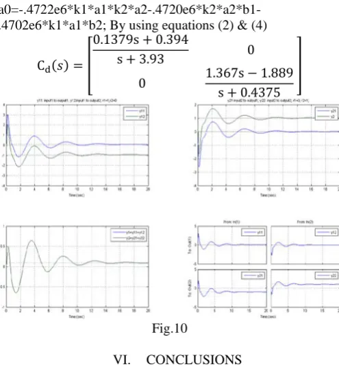
a0=-.4722e6*k1*a1*k2*a2-.4720e6*k2*a2*b1-.4702e6*k1*a1*b2; By using equations (2) & (4) Cd(𝑠) =�
0.1379s + 0.394
s + 3.93 0
0 1.367ss + 0.4375−1.889�
Fig.10
VI. CONCLUSIONS
The resultant controller is: Implementable, Low Order, All Stabilizing and Robust. Only output feedback is used and all given closed loop specifications are satisfied.
Using CDM and GA robust PSS can be designed by choosing any operating point (in the specified range) as our nominal operating condition. The method is flexible to choose nominal operating point, where the plant is running most of the time, at which we desire better performance.
APPENDIX A. Open loop state space representation:
The state equation of a single machine connected with infinite bus (SMIB) system may be derived from the linearized transfer function model (Fig.2) as:
𝑥̇= A𝑥+𝑏𝑢 ∆𝜔=𝑐1𝑥
∆𝑉𝑡=𝑐2𝑥
Where,
𝐴=
⎣ ⎢ ⎢ ⎢ ⎢ ⎢ ⎢
⎡ 0 𝜔𝑟 0 0
−2𝑘𝐻1 −2𝐷𝐻 −2𝑘𝐻2 0
−𝑘4
𝜏𝑑0′ 0 −
1 𝑘3𝜏𝑑0′
1 𝜏𝑑0′
−𝐾𝑎𝑇𝑘5
𝑎 0 −
𝐾𝑎𝑘6
𝑇𝑎 −
1 𝑇𝑎⎦
⎥ ⎥ ⎥ ⎥ ⎥ ⎥ ⎤
𝑏=�0 0 0 𝐾𝑇𝑎
𝑎� 𝑡
𝑐1=[0 1 0 0]
𝑐2=[𝑘5 0 𝑘6 0]
State vector x is defined as, 𝑥=�∆𝛿 ∆𝜔 ∆𝐸𝑞′ ∆𝐸𝑓𝑑�𝑡 Where ∆𝛿, ∆𝜔, ∆𝐸𝑞′ and ∆𝐸𝑓𝑑 are the incremental changes in rotor speed, rotor angle, voltage proportional to field flux linkage and field voltage respectively. ki, i=1, 2… 6 are the k-parameters whose value depends on the operating conditions.
B. Equations for k-parameters [7]
𝑘1= KtV∞�𝐸𝑞𝑎�𝑅𝑒𝑠𝑖𝑛(𝛿 − 𝛼) +�𝑋𝑒+𝑥𝑑′� 𝑐𝑜𝑠(𝛿 − 𝛼)�
+𝐼𝑞�𝑥𝑞− 𝑥𝑑′���𝑋𝑒+𝑥𝑞� 𝑠𝑖𝑛(𝛿 − 𝛼)
− 𝑅𝑒𝑐𝑜𝑠(𝛿 − 𝛼) ��
𝑘2=𝐾𝑡�𝑅𝑒𝐸𝑞𝑎+𝐼𝑞�𝑅𝑒2+�𝑋𝑒+𝑥𝑞�2��
𝑘3=�1 +�𝐾𝑡�𝑥𝑞− 𝑥𝑑′��𝑋𝑒+𝑥𝑞��� −1
𝑘4=𝐾𝑡𝑉∞�𝑥𝑑− 𝑥𝑑′���𝑋𝑒+𝑥𝑞� 𝑠𝑖𝑛(𝛿 − 𝛼)
− 𝑅𝑒𝑐𝑜𝑠(𝛿 − 𝛼)�
𝑘5=𝐾𝑉𝑡𝑉∞ 𝑡 �𝑉𝑞𝑥𝑑
′�𝑅
𝑒𝑐𝑜𝑠(𝛿 − 𝛼)− �𝑋𝑒+𝑥𝑞� 𝑠𝑖𝑛(𝛿 − 𝛼)�
− 𝑉𝑑𝑥𝑞�𝑅𝑒𝑠𝑖𝑛(𝛿 − 𝛼)
+�𝑋𝑒+𝑥𝑑′� 𝑐𝑜𝑠(𝛿 − 𝛼)��
𝑘6=𝑉𝑉𝑞
𝑡�1− 𝐾𝑡�𝑋𝑒+𝑥𝑞�𝑥𝑑
′� −𝐾𝑡𝑉𝑑
𝑉𝑡 𝑅𝑒𝑥𝑞
Where
𝐾𝑡=𝑅 1
𝑒2+ (𝑋𝑒+𝑥𝑑′)�𝑋𝑒+𝑥𝑞�
C. System parameter values [2]
TABLE II SYSTEM PARAMETERS
H 𝜔𝑟 𝐾𝑎 𝑇𝑎 𝑅𝑒 r ∆𝑉𝑡 D
3.25 314.15 50 0.05 0 0 1 0
𝑥𝑑 𝑥𝑞 𝑥𝑑′ 𝜏𝑑0′
2.0 1.91 0.224 4.18
REFERENCES
[1]. Keel, L.H. and Bhattacharyya, S.P., “Robust, Fragile or Optimal?” IEEE Trans. Automat. Contr., vol. 42, no. 8, pp 1098-1105, August 1997.
[2]. Herbert Werner, Petr Korba, and Tai Chen Yang., “Robust Tuning of Power System Stabilizers Using LMI-Techniques”, IEEE Trans. On Control Systems Technology, vol.11, no.1, January 2003.
[3]. S. Manabe. “The Coefficient Diagram Method”, The 4P
th
P
IFAC Symposium on Automatic Cont. in Aerospace, Seoul, Korea, pp. 199-210, Aug. 1998.
[4]. M. T. Soylemez and N Munro, Robust Pole assignment in uncertain systems, Proc. IEE: Control Theory and Applications, 144(3), pp 217-224.
[5]. Barmish, B. R., “New Tools for Robustness of Linear Systems”, Macmillan Publishing Company, New York, 1994.
[6]. Heffron, W. G. and Philips, R. A., “Effect of a modern amplidyne voltage regulator on under-excited operation of large turbine generators”, AIEE Transactions, 71: 692-697, 1972.
[7]. Anderson, P.M and Fouad, A.A., “Power system control and stability”, Second Edition, A Wiley InterScience Publication, John Wiley and Sons Inc.
[8]. Rao, P.S. and Sen, I., “Robust tuning of power system stabilizers using QFT”, IEEE Trans. Control Systems Technology, vol. 7, no. 4, pp. 478-486, July 1999.
[9]. T.K Sunil Kumar and Jayanta Pal., “Robust tuning of power system stabilizers using Optimization Techniques”, IEEE international Conference, pages: 1143-1148, on 12-17 Dec 2006.
[10]. E.V. Larsen and D. A Swann, “Applying power system stabilizers (three parts),” IEEE Trans. Power Apparatus Syst., vol. PAS-100, pp. 3017-3046, 1981.
[11]. Hung.N.T and Anderson.B.D.O., “Triangulation Technique for the Design of Multivariable Control Systems,” IEEE Trans. Automat. Control, vol. AC-24, no.3, pp. 455-460, Nov. 1979.
[12].Chieh-Li Chen and Neil Munro, “Procedure to achieve diagonal dominance using a PI/PID controller structure,” International Journal of Control, vol. 50, no. 5, pp- 1771-1792, 1989.
[13]. P.D. McMorran, S.M., “Design of gas-turbine controller using inverse Nyquist method,” Proc.IEE, vol, 177, no.10, pp-2050-2056, 1970.
[14]. Morari, M, and Zafirion, E., Robust Process Control. Prentice Hall Inc., Eaglewood Cliffs, 1989.
[15]. Sinha, P. K., Multivariable Control: An Introduction. Marcel dekker, Inc. N.Y., 1984.
[16]. Shieh, I. S., Datta-Barua, M., and Yates, R. E., “A modified direct-decoupling method for multivariable conrol system designs,” IEEE Trans. on Industrial Electronics and Control Instrumentation, vol. IECI-28, no.1, pp. 1-9, 1981.
[17]. Vasu Puligundla and Jayanta Pal, "Robust Tuning of Power System Stabilizers Using Coefficient Diagram Method", International Journal of Electrical Engineering, ISSN 0974-2158 Volume 7, Number 2 (2014), pp. 257-270.