Novel Multi-Target Tracking Algorithm for Automotive Radar
Xun Gong, Ze-Long Xiao*, and Jian-Zhong Xu
Abstract—Tracking multiple maneuvering targets for automotive radar is a vital issue. To this end, a novel DS-UKGMPHD algorithm which combines diagraph switching (DS), unscented Kalman (UK) filter and Gaussian mixture probability hypothesis density (GMPHD) filter is proposed in this paper. The algorithm is capable of tracking a varying number of target cars detected by automotive radar with nonlinear measurement models in a cluttered environment. In addition, variable structure is used to accommodate various target motions in real world. Simulation results demonstrate the superiority of the presented algorithm to IMM-UKGMPHD filter in terms of estimation accuracy of both number and states.
1. INTRODUCTION
Accuracy and timeliness constitute two significant factors for automotive radar. Accordingly, the main goal of this paper is to track multiple targets detected by automotive radar, in other words, to estimate the number and positions of the detected vehicles reliably and timely and thereby reducing false alarm rate and reaction time in cluttered road environment.
To this end, two kinds of algorithms are introduced by relevant documental materials. Classic solution [1, 2] to multi-target tracking for automotive radar involves data association, track management and single-target Bayesian filtering. However, data association algorithms suffer from intensive computation burden, especially when the number of targets gets large. Another solution to multi-target tracking for automotive radar is based on Random Finite Set (RFS) theory, namely the popular probability hypothesis density (PHD) filter [3], with both Gaussian mixture PHD (GMPHD) filter [4] and Sequential Monte Carlo PHD (SMC PHD) filter [5–7] as implementations, and cardinalized PHD (CPHD) filter [8], tracks targets with a varying number without data association or target management. Considering the timeliness, the GMPHD filter is a suboptimal but computationally tractable alternative. It recursively propagates the first-order moment of the multi-target posterior [9]. Whereas problems exist in this filter: firstly, automotive radar tracks the targets in polar coordinates, which makes measurement equations nonlinear in Cartesian coordinates. Secondly, one single model can hardly describe real-world maneuvering targets. In view of these demerits, the IMM-GMUKPHD filter was proposed [10]. However, only two models are used in [10]. When more models are taken into account, the IMM algorithm featuring a fixed model set structure can lead to a dilemma: On one hand, a large model set may cover various behaviors of the cars. On the other hand, for a certain motion, a large set of models leads to heavy computation load and accuracy reduction.
To overcome the contradiction, a hybrid algorithm, whose framework is based on graph-theoretic MM approach, is proposed in this paper. Combining unscented probability hypothesis density filter with diagraph switching (DS) [11], a variable structure multiple model algorithm, the presented algorithm determines certain subset of the total model-set in real time before IMM-UKGMPHD algorithm is implemented.
Received 18 December 2015, Accepted 3 February 2016, Scheduled 10 February 2016
* Corresponding author: Zelong Xiao ([email protected]).
The layout of this paper is as follows. In Section 2, the problem of multi-target tracking for automotive radar is formulated. Section 3 describes the DS-UKGMPHD filter in detail. Simulation and discussion are given in Section 4. Finally, concluding remarks are presented in Section 5.
2. PROBLEM FORMULATION
In the application of an anti-collision system, target vehicles in front of the radar carrying vehicle are detected. Generally, the motion of the ith target in the xy-plane can be described as
xik=Fk,mi (xik−1) + Γkwik,m (1)
where Γk =
⎡ ⎢ ⎢ ⎢ ⎢ ⎢ ⎣
T2/4 0
T/2 0
0 T2/4 0 T/2
1 0 0 1 ⎤ ⎥ ⎥ ⎥ ⎥ ⎥ ⎦
is the input matric. xik = [x,x, y,˙ y,˙ x,¨ y¨]T denotes the six-dimensional
state vector of the target at timekT (k is the time index andT is the sampling interval). The variables (x, y), ( ˙x,y˙) and (¨x,y¨) in the state vector xik represent the target position, velocity and acceleration in the x and y directions respectively. The process noise wik,m is a vector of input white noise with zero mean, wkmi ∼ N(0, Q), where Q denotes the process noise covariance. m represents the index of the models. The state transition matrices are defined as
Fl k,φ = ⎡ ⎢ ⎢ ⎢ ⎢ ⎢ ⎣
1 sinω/ω 0 −(1−cosω)/ω 0 0 0 cosω 0 −sinω 0 0 0 (1−cosω)/ω 1 cosω 0 0
0 sinω 0 cosω 0 0
0 0 0 0 1 0
0 0 0 0 0 1
⎤ ⎥ ⎥ ⎥ ⎥ ⎥ ⎦ (2) Fi k,5 = ⎡ ⎢ ⎢ ⎢ ⎢ ⎢ ⎣
1 T 0 0 T2/2 0
0 1 0 0 T 0
0 0 1 T 0 T2/2
0 0 0 1 0 T
0 0 0 0 1 0
0 0 0 0 0 1
⎤ ⎥ ⎥ ⎥ ⎥ ⎥ ⎦ (3)
The matrixFk,ϕl (·) denotes the Constant Turn (CT) model. We choose ϕ= 1,2,3,4 with different turning rates ω = −1 rad/s, −0.05 rad/s, 0.05 rad/s, 1 rad/s respectively to describe the motions of lane-changing. Fk,5i , the Constant Acceleration (CA) model, describes linear motion with a uniform acceleration and constant speed.
The noisy measurement vectorzki, which includes the bearingθki and range measurementsrki of the
ith target at timekT, is defined as
zki =
θi k ri k = ⎡ ⎢ ⎢ ⎣ arctany i k−ys,k xi
k−xs,k
xi k−xs,k
2
+yik−ys,k2
⎤ ⎥ ⎥ ⎦+ vi θ,k vi r,k (4)
where the measurement noise [viθ,k, vir,k]T is a 2×1 zero-mean Gaussian noise vector with covariance matrixR.
3. PROPOSED DS-UKGMPHD FILTER
Step 1: Initialize a diagraph set.
Here Φ is chosen to be the total diagraph and Φ(l){βl−1, βl, βl+1} is the stochastic sub-diagraph. l is the model index. Markov chain with transition probability matrix is πpq. Φ(0) is considered
as the default sub-diagraph. Here the graphic presentation Φ for automotive radar is as shown in Fig. 1.
Figure 1. Diagraph Φ for targets detected by automotive radar.
Step 2: Set up an effective logic to instruct the transition of models.
Suppose that the sub-graph is Φ(k−1) at sampling timek−1, the decision rule is
Φ(k)=
⎧ ⎪ ⎪ ⎨ ⎪ ⎪ ⎩
Φ(l−1), if μ(lk−−11) > τDS
Φ(l+1), if μ(l+1)k−1 > τDS
Φ(l), otherwise
(5)
where τDS is a threshold probability for mode transition, and μ(lk−±11) denotes the probability of β(l±1) at sampling time k−1.
Step 3: Initialization and mixing for certain sub-diagraph.
Fork= 0, initiate each state target ˆX0q, the covariance matrix ˆP0qand model probabilityμq0 = 1/M.
M is the number of the models in the model-subset, here we choose M = 3 as Fig. 1 indicates. The current model index isq(q= 1, . . . , M).
(1) Fork=k+ 1, k >0
μ(i)k−1,pq=
1 ¯
cqπpqμ i
k−1,p (6)
where
c(i)k−1,q =
M
p=1
πpqμ(i)k−1,p (7)
μ(i)k−1,pis the occurrence probability of theith target using modelp. The initial mixed PHD function
Dk−1,q(x) = M
p=1
Dk−1,p(x)μ(i)k−1,pq (8)
The mixed weight, state, and covariance matrix are respectively as follows.
ω(i)k−1,q = M
p=1
ωk(i)−1,pμ(i)k−1,pq (9)
˜
Xk(i)−1,q =
M
p=1
ˆ
Pk(i)−1,q = M
p=1
μ(i)k−1,pq
Pk(i)−1,p+ςk(i)−1,pq
ςk(i)−1,pq
T
(11)
where
ςk(i)−1,pq= ˆXk(i)−1,p−X˜k(i)−1,q (12)
Step 4: Run the UKGMPHD filter for each model.
ωk(i)−1,q, ˜Xk(i)−1,q and Pk(i)−1,q above-mentioned are inputs of the UKGMPHD filter. The steps include
prediction, updating, pruning and merging [12]. Unscented transition is used in prediction and updating steps. The estimation results areωk,q(i), ˜Xk,q(i) andPk,q(i).
Step 5: Update of the model probabilities.
The likelihood and probability of the ith Gaussian component based on modelq at the sampling timekare respectively as follows.
Λ(i)k,q = N
Zk|q,X˜k(i)−1,q,P˜k(i)−1,q
(13)
μ(i)k,q = 1
c(i)Λ (i) k,q
M
p=1
πpqμ(i)k−1,p (14)
Step 6: Combined estimation. The combined PHD function is
Dk(x) = M q=1 Jk i=1 ωk,q(i)N
x,X˜(i)
k,q, Pk,q(i)
(15)
whereJk is the number of the Gaussian components.
The combined weight, state, and covariance matrix are respectively as follows.
ωk(i) = M
q=1
ωk,q(i)μ(i)k,q (16)
ˆ
Xk(i) = M
q=1
ˆ
Xk,q(i)μ(i)k,q (17)
Pk(i) =
M
q=1
μ(i)k,qPk,q(i)+ς(ς)T
(18)
where
ςk,pq(i) = ˆXk(i)−X˜k,q(i) (19)
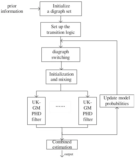
The flow diagram for DS-UKGMPHD filter is presented in Fig. 2.
4. SIMULATION AND DISCUSSION
4.1. Simulation Scenario and Parameter Setting
In this section, a Cartesian two-dimensional scenario is presented. Both DS-GMUKPHD filter and IMM-GMUKPHD filter are then used to track these targets for comparison. The sample interval is 0.1 s, and the total simulation time is 10 s. Assuming that the maximum measurement range of the radar is 120 m, the test scenario is constructed as follows:
prior information
output
Initialize a digraph set
Set up the transition logic
diagraph switching
Initialization and mixing
UK-GM PHD filter
UK-GM PHD filter ĂĂ
Update model probabilities
Combined estimation
Figure 2. Flow diagram for DS-UKGMPHD filter.
Table 1. Simulation parameters.
Simulation Parameters parametric meanings Value
τDS threshold for sub-graph transition 0.65
Ps targets’ survival probability 0.95 PD targets’ detection probability 0.99
τ pruning threshold 10−5
Umerge merging threshold 4
Jmax maximum number of Gaussian components 100
r Poisson means 4
Q process noise covariance diag([5,2,5,2,0.5,0.5])
R measurement noise covariance diag([0.01,0.01])
this car. Target 1 keeps linear motion with the initial state x10 = [62,0,120,−0.2,0,−0.2]T during [0.1,1.2] s, and keeps linear motion with a uniform acceleration of 0.08 m/s2 during [1.3,4] s. After
that, it keeps linear motion at a constant speed; Target 2 changes lanes for two times: it turns right with initial statex2
0 = [70,−2.8,106,−2.7,0,0]T and a turn-rate ofω =−0.1 rad/s during [2.1,3.6] s,
and then changes back to the lane with a turn-rate of ω = −0.04 rad/s. Target 3 has an initial state of x30 = [22,0,3,1.7,0,0.5]T during [3.1,4.5] s and then keeps linear motion with a uniform acceleration of−0.02 m/s2; target car 4 is detected with initial statex40 = [18,0,3,2.5,0,0]T since 6 s and start to change the lane 0.8 s later. The turning rates are 0.05 rad/s,−0.05 rad/s respectively. During the simulation steps [9.3, 10] s, the car moves with a constant velocity of 27.5 m/s.
sub-models is set by πpq =
0.75 0.125 0.125
0.125 0.75 0.125 0.125 0.125 0.75
, simulation parameters are listed in Table 1.
4.2. Simulation Results and Discussion
Figure 3 shows the true trajectories of four targets detected by automotive radar and the measurements which originate from either targets or clutter. In Fig. 4 and Fig. 5, tracking results based on the DS-UKGMPHD filter and IMM-DS-UKGMPHD filter against the true tracks are shown. The automotive radar is located at the pentagram marker, and each trajectory starts at the circle markers. The individual
x and y coordinates of real tracks and estimations for each time step are shown in Figs. 6 and 7. The estimated number of targets based on the two algorithms against true values is plotted in Fig. 8 and the optimal sub-pattern assignment (OSPA) distance (p= 2, c= 8) at each time step is illustrated in Fig. 9 for further evaluation.
First, it can be found that the estimated positions based on DS-UKGMPHD filter are close to the true tracks in Fig. 4 and Fig. 6, whereas the estimated positions based on IMM-UKGMPHD filter are comparatively undesirable, which can be illustrated by two obviously incorrect positions at 2.1 s and 7.4 s in Fig. 7. Second, in Fig. 8, the IMM-UKGMPHD filter estimates the target number wrongly
Figure 3. Measurements of the detected cars in the clutter.
Figure 4. Multi-target tracking for automotive radar using DS-UKGMPHD.
Figure 6. Targets’ positions within the measurement time using DS-UKGMPHD.
Figure 7. Targets’ positions within the measurement time using IMM-UKGMPHD.
Figure 8. Targets’ number estimated by DS-UKGMPHD and IMM-DS-UKGMPHD.
Figure 9. OSPA distance based on
DS-UKGMPHD and IMM-DS-UKGMPHD.
for five times (at 2.1 s, 3.2 s, 3.3 s, 6.1 s and 7.4 s), while DS-UKGMPHD filter misestimates for once. Third, Fig. 9 shows that the OSPA values of two filters peak correspondingly at the instances where the estimated number is incorrect. When the estimated number of targets is correct, the OSPA miss-distance of the DS-UKGMPHD filter proves smaller than IMM-UKGMPHD filter.
5. CONCLUSION
ACKNOWLEDGMENT
This paper was supported by the National Natural Science Foundation of China (No. 61301213).
REFERENCES
1. Wang, H. and J. Liu, “The analysis of target track of passive radar based on Kalman filter,”Tactical Missile Technology, 2005.
2. Kim, B., K. Yi, H. J. Yoo, H. J. Chong, and B. Ko, “An IMM/EKF approach for enhanced multi-target state estimation for application to integrated risk management system,”IEEE Transactions on Vehicular Technology, Vol. 64, No. 3, 1, 2014.
3. Mahler, R. P. S., “Multitarget bayes filtering via first-order multitarget moments,” IEEE Transactions on Aerospace &Electronic Systems, Vol. 39, No. 4, 1152–1178, 2003.
4. Lundquist, C., L. Hammarstrand, and F. Gustafsson, “Road intensity based mapping using radar measurements with a probability hypothesis density filter,” IEEE Transactions on Signal Processing, Vol. 59, No. 2, 1397–1408, 2011.
5. Heuer, M., A. Al-Hamadi, A. Rain, and M. M. Meinecke, “Detection and tracking approach using an automotive radar to increase active pedestrian safety,” 2014 IEEE Intelligent Vehicles Symposium Proceedings, 890–893, IEEE, 2014.
6. Hong, S., L. Wang, Z.-G. Shi, and K. S. Chen, “Simplified particle phd filter for multiple-target tracking: Algorithm and architecture,” Progress In Electromagnetics Research, Vol. 120, 481–498, 2011.
7. Chen, J.-F., Z.-G. Shi, S.-H. Hong, and K. S. Chen, “Grey prediction based particle filter for maneuvering target tracking,” Progress In Electromagnetics Research, Vol. 93, 237–254, 2009. 8. Georgescu, R. and P. Willett, “The multiple model CPHD tracker,” IEEE Transactions on Signal
Processing, Vol. 60, No. 4, 1741–1751, 2012.
9. Maher, R., “A survey of PHD filter and CPHD filter implementations,” Proceedings of SPIE — The International Society for Optical Engineering, Vol. 6567, 65670O–65670O-12, 2007.
10. Hao, Y. L., F. B. Meng, F. Sun, and F. Shen, “Application of UK-GMPHDF algorithm based on imm in multiple maneuvering targets tracking,” Systems Engineering — Theory & Practice, Vol. 31, No. 11, 2225–2233, 2011.
11. Li, X. R. and Y. Bar-Shalom, “Multiple-model estimation with variable structure,” IEEE Transactions on Automatic Control Ac, Vol. 41, No. 4, 478–493, 1996.