Software Analysis Techniques For Odor Analysis and Classification Using the Electronic Nose

Abstract

GAYO, JAVIER. Software Analysis Techniques for Odor Analysis and Classification Using the Electronic Nose. (Under the direction of Dr. Susan M. Blanchard and Dr. S. Andrew Hale.)

The objectives of this thesis were to compare methods of feature extraction and data classification used in electronic nose. The NC State electronic nose (e-nose) was used to discriminate between SkipJack tuna (Katsuwonus pelamis) samples cooked at three temperatures: raw, heated to 55°C, and heated to 85°C. The thirty-six samples

SOFTWARE ANALYSIS TECHNIQUES FOR ODOR ANALYSIS AND CLASSIFICATION USING THE ELECTRONIC NOSE

by

JAVIER GAYO

A thesis submitted to the Graduate Faculty of North Carolina State University

in partial fulfillment of the requirements for the Degree of

Masters of Science.

BIOLOGICAL AND AGRICULTURAL ENGINEERING

Raleigh 2002

APPROVED BY:

_____________________________ ______________________________ Dr. Susan M. Blanchard Dr. S. Andrew Hale Co-Chair of Advisory Committee Co-Chair of Advisory Committee

ACKNOWLEDGEMENTS

I would like to thank several individuals who have made my graduate studies, here at North Carolina State University, a learning experience. I would like to express my deepest thanks to the Co-Chairs of my committee, Dr. Susan M. Blanchard and Dr. S. Andrew Hale. I could not have made it this far without your support and encouragement. Thanks for all the helpful advice you have given me. Thanks to Dr. Peter L. Mente for the ideas and advice on how to improve my thesis.

BIOGRAPHY

TABLE OF CONTENTS

List of Tables ………..vi

List of Figures ……… vii

List of Nomenclature ………. viii

1 Introduction... 1

1.1 The Significance and Importance of Smell... 1

1.2 The Biology of Smell... 1

1.3 Odor Evaluation in the Food Industry ... 2

1.3.1 Human Panels ... 3

1.3.2 Gas Chromatography (GC) and Mass Spectrometry (MS)... 3

1.4 The Making of an Electronic Nose ... 4

1.4.1 The Anatomy of an Electronic Nose... 4

1.4.2 Electronic Olfaction... 5

1.5 Electronic Noses in the Food Industry... 6

1.6 Other Applications of Electronic Noses ... 6

1.7 Thesis Objectives ... 7

2 Methods of Feature Extraction... 9

2.1 Principal Component Analysis ... 9

2.2 Linear Discriminant Analysis ... 13

3 Classification Algorithms ... 16

3.1 Least Squares ... 16

3.2 K-Nearest Neighbor ... 19

3.3 Artificial Neural Networks ... 20

3.3.1 Single Layer Networks: The McCulloch-Pitts Neuron, the Perceptron, and the Adaline ... 21

3.3.2 The Delta Rule ... 24

3.3.3 Multi-layered Networks and the Backpropagation Algorithm ... 25

3.3.4 The Generalized Delta Rule... 30

3.3.5 Momentum... 31

4 Materials and Methods... 32

4.1 The NC State Electronic Nose ... 32

4.2 Preparation of SkipJack Tuna Samples... 34

4.3 Data Analysis ... 35

5 Results and Discussion ... 37

5.1 Feature Extraction Methods... 37

5.2 Data Classification Algorithms... 43

6 Conclusion and Recommendations... 53

LIST OF TABLES

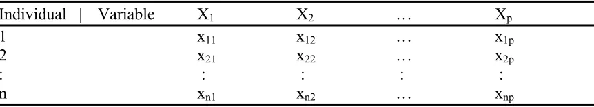
Table 2-1: Data Layout for PCA... 10

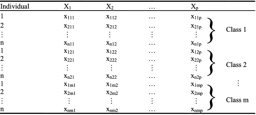
Table 2-2: Data Layout for LDA………..13

Table 4-1: Cross Sensitivities of the Sensors Used in the NC State E-nose... 32

Table 5-1: Comparison of Classification Percentages, Mean (Standard Deviation). ... 44

Table 5-2: Topology and Parameters Used in the ANN. ... 48

Table 5-3: Classification Criteria for the Testing Data of the ANN... 49

LIST OF FIGURES

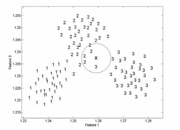
Figure 3-1: Visualization of the K-Nearest Neighbor Method. ... 19

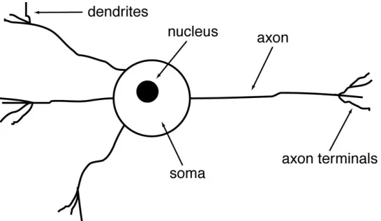
Figure 3-2: The Components of a Biological Neuron ... 20

Figure 3-3: The Artificial Neuron - the McCulloch-Pitts Neuron. ... 22

Figure 3-4: The Two-Phase Procedure for a Backpropagation Neural Network... 27

Figure 3-5: The Graph of the Logistic Sigmoid Function. ... 29

Figure 4-1: Flow Diagram of the NC State E-nose... 33

Figure 5-1: LDA Projections for Treatment Classification. ... 38

Figure 5-2: PCA Projections for Treatment Classification... 39

Figure 5-3: PCA Graph Showing Discrimination Among Days of E-nose Analysis... 40

Figure 5-4: Second (PC2) and Third (PC3) Principal Components. ... 42

Figure 5-5: PC2 and PC3 Taking Into Account Only Day of E-nose Analysis... 42

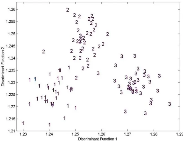
Figure 5-6: LDA Training and Testing Sets Based on Treatment. Numbers with an Asterisk (*) Represent Test Data. ... 45

LIST OF NOMENCLATURE Xp: pth variable

xip: value of ith individual for the pth variable PCi: ith principal component

DFi: ith discriminant function aij: values of eigenvector a

cjk: covariance between variables j and k

λi: eigenvalues of a covariance matrix

B: between-sample matrix W: within-sample matrix T: total sample matrix

w: value of interlayer weights

E: squared error of the difference between a desired output and the actual output I: denotes the actual output of a neuron

f(I): output of a neuron after going through a transfer function, i.e. sigmoid

δ: error of a neuron used in backpropagation

1 Introduction

1.1 The Significance and Importance of Smell

The sense of smell (olfaction) is probably the most important of the senses to a large number of animal species on Earth. In mammals and humans, it functions to signal pleasure, avoidance, sexual attraction, and even recognition (Farbman, 1992;

Strassburger, 1997). Physicians are able to classify diseases, such as pneumonia, by the odor of the patient’s breath or bodily fluids. Most importantly, however, is the role of olfaction in the food industry. Olfaction is one of the three senses that contributes to the sensation of flavor. Gustation (taste) and the trigeminal sense (important in detecting irritating chemical compounds) are the other two (Dodd et al., 1992; Gardner and Bartlett, 1994). The hundreds of volatile organic compounds (VOCs) that make up a food product’s aroma define the nature and identity of that food product (Hodgins, 1997). The food industry relies heavily on the aroma of their products because aroma contributes to consumer preferences among types and brands of food products.

1.2 The Biology of Smell

The odorant molecules that make up an odor are generally small (20-300 Daltons), hydrophobic, and polar. Human smell begins with the simple action of

sniffing, which moves the air, along with odor molecules, through a series of curved bony structures called turbinates (Farbman, 1992). These structures create turbulent airflow patterns, thus mixing and carrying the VOCs to the thin mucus coating surrounding the nose’s olfactory epithelium. The VOCs making up the odor reach the olfactory

to the epithelium, which contains sensory cells. The sensory neurons in the epithelium have cilia (hair-like structures) with receptors on their outer membrane. Roughly one thousand different kinds of receptor cells are distributed throughout the olfactory epithelium (Strassburger, 1997). When the VOCs bind to the receptors of the sensory cells, the integration of information from the receptors, which occurs in the brain, creates the perception of smell.

After the odorant molecule binds to the receptors, enzymatic reactions cause depolarization of the sensory cell’s membrane, which creates a signal along its axon (Farbman, 1992). The axon of the cells and the signal reach the olfactory bulb located in the brain. The olfactory bulb is composed of glomeruli (a cluster of neural networks), mitral cells, and a granular layer (Bartlett et al., 1997). The first unit of odor information processing occurs at the glomeruli where similar receptors of a particular type converge to a specific group of glomeruli. The receptor stimulation results in a two-dimensional topographical map representing the odor. The electrical signals processed by the mitral cells are sent via the granular layer to the hypothalamus where the neural signals of gustation are also processed. Although the actual path of sensory information is

unknown, it is believed that it finally reaches the temporal lobe of the cerebral cortex of the brain where the odor is classified and memorized. Studies based on noninvasive techniques suggest that different chemical stimuli activate different regions of the brain.

1.3 Odor Evaluation in the Food Industry

Bartlett, 1994). Traditional methods of measuring odors in the food industry include organoleptic tests (human odor panels), gas chromatography, and mass spectrometry tests.

1.3.1 Human Panels

Human panels are the primary method for evaluating product quality (Dodd et al., 1992). This method, however, is far from perfect, expensive, and time-consuming. The main problem is due to odor fatigue as the receptor cells become saturated and

desensitized by the odor. Thus, the humans in the panel can only work for short periods of time. Studies have also demonstrated the presence of anosmia (inability to smell particular odors), hyposmia (reduced sensitivity of the olfactory system), and parosmia (distortion in odor perception) (Farbman, 1992; Gardner and Bartlett, 1999). This can affect the evaluation of a product and lead to misclassification. Other problems include health risks associated with smelling certain chemical compounds or products, such as mold spores in grain (Borjesson et al., 1996), and variation of detection of odors due to age, sex, health, and diet (Dodd et al., 1992; Hodgins, 1997).

1.3.2 Gas Chromatography (GC) and Mass Spectrometry (MS)

(sweet, pungent, etc.) (Gutierrez-Osuna, 1998). Therefore, the main drawback to these techniques is the inability to compare the results of GC and MS tests to human odor perception.

1.4 The Making of an Electronic Nose

The need for an electronic instrument that mimics the sense of olfaction has grown over the past few decades due to the drawbacks in the traditional methods used to evaluate food quality (Gardner and Bartlett, 1994). Even though the development of an instrument capable of detecting odors dates back to Moncrieff (1961), the first electronic nose was not developed until almost two decades later. In 1982, Persaud and Dodd first reported their research on an electronic instrument capable of discriminating between simple and complex odors. The term “electronic nose” itself did not emerge until 1987 when it was specifically used at a conference to refer to an electronic instrument used to detect and discriminate between odors. Collins and Moy (1995) defined the term as “an instrument capable of mimicking at least some of the functionality of the human sense and should be able to detect both simple and complex odours.”

1.4.1 The Anatomy of an Electronic Nose

Electronic noses (e-noses) are comprised of an array of sensors, signal

transduction circuitry, and a pattern recognition system (Gardner and Bartlett, 1994). As an analogy to the human nose, the sensor array represents the sensory cells in the

reaching the brain. This circuitry also compresses the signals and amplifies the output in order to reduce noise and improve sensor sensitivity (Craven et al., 1996). The last part comprising an electronic nose, the pattern recognition system, represents the cerebral cortex of the brain (Hodgins, 1997).

1.4.2 Electronic Olfaction

Generally, headspace gases from a sample are pumped through the sensor array by a vacuum pump (Nagle et al., 1998). The number of sensors in the array can vary. Studies have been made with electronic noses containing 6, 12, and 18 sensors (Collins and Moy, 1995). The sensors in the array measure a change in resistance due to the presence of chemical compounds (VOCs) in the air sample (Gutierrez-Osuna, 1997). These compounds change the oxygen concentration over the sensors by absorbing or producing oxygen. The change in oxygen concentration causes a change in the resistance (∆R) across each sensor, which is converted to a change in voltage (∆V) via a

Recently, artificial neural networks (ANNs) have also been used in odor classification techniques.

1.5 Electronic Noses in the Food Industry

The main application of electronic noses has been geared towards the food industry. Maul et al. (1999) did a study to explore the effects of harvest maturity and storage temperature of ripe tomatoes on their volatile profiles. Pardo et al. (1999) used an electronic nose to discriminate between different types of cheese. Korel et al. (1999) concluded that the electronic nose was able to correlate milk aroma with microbial load and storage time. In a similar study, Magan et al. (2001) used an electronic nose to recognize spoilage bacteria and yeasts in milk and concluded that it might be a useful tool in early detection of dairy spoilage. Research has also been done to evaluate the

electronic nose for use in the meat industry (Braggins et al., 1999), detect odor and microbial evaluation of raw tuna (Newman et al., 1999), evaluate decomposition aroma in raw and cooked shrimp (Luzuriaga and Balaban, 1999), distinguish between “good” and “bad” dry cured hams (Abass et al., 1999), and discriminate among cocoa beans roasted at different temperatures (Hashim and Plumas, 1999).

1.6 Other Applications of Electronic Noses

bacterial populations living at the skin surface. Since commonly diagnosed human diseases produce a distinctive body odor, this study focused on the possibility of using an e-nose to analyze chemical emissions and aid in disease diagnosis. In a similar study, Gardner et al. (2000a) used an electronic nose to identify pathogens from cultures and diagnose illness from breath samples. Ehrmann et al. (2000) evaluated human breath odor to detect the gaseous components of bad breath.

E-noses have also been used to monitor environmental conditions (Baby et al., 2000). In this study, the e-nose was able to discriminate between lindane and

nitrobenzene, two water contaminants in low concentrations (1 and 500 ppm,

respectively). It was also able to discriminate among insecticides (synthetic pyrethroids), odorless to human panels, in small quantities (60 mg). Lee et al. (2000) were able to effectively identify explosive gases such as methane, propane, and butane. Other studies of e-nose applications include the identification of Forane R134a (a refrigerant gas) under controlled gas temperature and humidity conditions (Delpha et al., 2000), successful discrimination between five different polyurethane foams used in car seat manufacturing (Morvan et al., 2000), assignment of unknown malodors to environmental sources (Nicolas et al., 2000), and the monitoring of potable water quality (Gardner et al., 2000b).

1.7 Thesis Objectives

safety and product evaluations. Such evaluations primarily focus on sensory evaluations, microbial counts, and the presence of histamine (Newman et al., 1999). Low microbial counts and absence of histamine, however, do not ensure that the tuna is of high quality or safe to consume. Results from sensory evaluations are also often influenced by factors such as age, health, gender, and odor fatigue of the evaluators (Hodgins, 1997).

Electronic nose technology has been used to objectively evaluate fresh food products, such as tuna.

Prior to canning for human consumption, pre-cooking is done to cause a texture change in tuna meat (Zang et al., 2001). This change helps workers separate the light tuna meat, the part used for canning for human consumption, from the rest of the fish. The texture change is primarily caused by protein denaturation. Two major protein denaturation peaks occur at temperatures of 55ºC and 85ºC. The NC State University e-nose was used to attempt to distinguish aroma at these two temperatures as well as the aroma of raw SkipJack tuna (Katsuwonus pelamis). The objectives of this study were to:

1. Use the e-nose to classify samples into treatment groups (raw, heated to 55ºC, and heated to 85ºC).

2. Compare Principal Component Analysis (PCA) and Linear Discriminant Analysis (LDA) as feature extraction methods.

2 Methods of Feature Extraction

Feature extraction methods transform the dimensionality of a data set, M, into a feature space, N, of lower dimension (N<M). The features obtained preserve as much of the information contained in the original set as possible. This section describes two common methods of feature extraction: principal component analysis (PCA) and linear discriminant analysis (LDA). In general, the extracted features are often referred to as “features.” In the following sections, however, the features will have names descriptive of the feature extraction method. Features in PCA will be referred to as Principal Components (PC) and the features in LDA as Discriminant Functions (DF).

2.1 Principal Component Analysis

PCA is a linear and unsupervised multivariate statistical method that reduces the dimensionality of a multivariate problem to allow the information to be represented in a 2-D or 3-D graph (Flury, 1988; Gardner and Bartlett, 1992). The term unsupervised refers to lack of information on the samples prior to attempting to find a relationship. Therefore, this technique is useful when hidden relationships among samples are suspected. Uses of PCA include noise reduction, data compression, feature extraction, and visualization of high dimensional data. Simply put, PCA transforms a large set of correlated data (a relationship, usually linear, exists among the data) into smaller sets of uncorrelated data (there exists no relationship among the data) that represent the original set (Manly, 1986).

uncorrelated features called principal components (PCs) (Manly, 1986). The xnp in Table 2-1 represent the actual values of the individuals for the corresponding variable. For example, x12 represents the value of the first individual for the second variable. Due to the lack of correlation, the PCs measure different dimensions in the data set. The principal components are ordered in decreasing order of importance so that var(PC1) > var(PC2) > ... > var(PCp), where var(PCi) denotes the variance of the PCi in the original data set. In other words, PC1 represents the largest amount of variation and PCp the least (Jolliffe, 1986). In many instances, the variation is low enough to be negligible;

therefore, the data set can be adequately represented by a few principal components. A data set containing 20 or 30 variables, for example, can often be properly represented by only two or three principal components. In order for PCA to work efficiently, however, the original data needs to be correlated, and the higher the correlation (regardless of whether it is positive or negative) the better. If, on the other hand, the original data are uncorrelated, PCA will generate useless results.

Table 2-1: Data Layout for PCA.

Individual | Variable X1 X2 … Xp

1 x11 x12 … x1p

2 x21 x22 … x2p

: : : : :

n xn1 xn2 … xnp

PCi = Σ(aijXj) (i = 1, ... , n; j = 1, ... , p) [2-1]

Where PCi = the ith principal component X = the variables under study a = values of eigenvector a

The principal components derived from equation 2-1 have the following constraints:

1) Σa2

ij = 1 [2-2a]

2) All of the PCiare uncorrelated. [2-2b] For example, the first principal component (PC1) is a linear combination of the variables X1, X2, ..., Xp. Using Table 2-1, the first PC is found by equation 2-3:

PC1 = a11x11 + a12x12 + a13x13 + ... + a1px1p [2-3]

The variance of PC1, var(PC1), is as large as possible given the constraint by equation 2-2a:

a211+ a212 + a213 + ... + a21p = 1 [2-4]

This constraint limits the value of var(PC1) to avoid making it larger by increasing any of the a1j constants in equation 2-3. The remaining principal components can be found by using equation 2-1 and applying the constraints of equations 2-2a and 2-2b.

              = pp p p p p c c c c c c c c c A Cov ... ... ... ) ( 2 1 2 22 21 1 12 11 M M M M [2-5]

Where the elements in the diagonal (cjj = sj2) represent the variance of Xj and the rest (cjk) represent the covariance between variables Xj and Xk. The formulas for the sample variance and covariance respectively are as follows:

(

)

∑

1 [2-6]

Where sj2= sample variance

xij = value of ith individual of the jth variable

j

x = sample mean of jth variable

n = sample size

(

)

(

)

∑

Where cjk = covariance between variables j and k xik = value of ith individual of the kth variable

k

x = sample mean of kth variable

The eigenvalues of Cov(A), λi, represent the variances of the principal components

(var(PCi) =λi), some of which may be zero. In other words, the ith eigenvalue

corresponds to the ith principal component:

An important property is the fact that the sum of the variances of the original variables is equal to the sum of the variances of the principal components. In other words, the trace of A (the sum of the diagonal elements) is equal to the sum of the eigenvalues. Due to this equality, the principal components account for the variation in the original data set.

2.2 Linear Discriminant Analysis

Linear Discriminant Analysis, first introduced by Fisher (1936), reduces the dimensionality of a multivariate problem while maximizing the separability between classes (Manly, 1986). LDA assigns an individual sample to a group based on data related to the group (Lachenbruch and Goldstein, 1979). LDA is done on p variables (X1, X2, … , Xp) for m samples belonging to different classes of size n (Table 2-2), and

determines linear combinations of the variables that separate the groups as much as possible (Manly, 1986). Each linear combination, known as canonical discriminant functions, takes the following form:

p ip i

i

i a X a X a X

DF = _{1 1}+ _{2 2}+_L+ [2-11]

In contrast to PCA, the data do not need to be standardized to have means of zero and variances of one because the outcome of the analysis is not significantly affected by the scaling of the variables. As is true in PCA, however, the first few discriminant functions usually account for the majority of the important group differences. A

graphical representation can then be used to describe group relationships by plotting the first two or three discriminant functions. The number of discriminant functions that LDA returns depends on the number of variables in the study and the number of classes minus one. The smaller of these two values indicates the number of discriminant functions that LDA returns.

LDA manipulates three matrices: W, the within sample matrix; B, the between sample matrix; and T, the total sample matrix (Manly, 1986). The elements of row r and column c of matrices T and W, respectively, are found using equations 2-12 and 2-13:

Individual X1 X2 … Xp

1 x111 x112 … x11p

2 x211 x212 … x21p

}

M M M M M

n xn11 xn12 … xn1p

1 x121 x122 … x12p

2 x221 x222 … x22p

M M M M M

n xn21 xn22 … xn2p

1 x1m1 x1m2 … x1mp

2 x2m1 x2m2 … x2mp

M M M M M

n xnm1 xnm2 … xnmp

}

}

Individual X1 X2 … Xp

1 x111 x112 … x11p

2 x211 x212 … x21p

}

M M M M M

n xn11 xn12 … xn1p

1 x121 x122 … x12p

2 x221 x222 … x22p

M M M M M

n xn21 xn22 … xn2p

1 x1m1 x1m2 … x1mp

2 x2m1 x2m2 … x2mp

M M M M M

n xnm1 xnm2 … xnmp

(

)(

)

rc x x x x

t

j

− −

=

∑∑

=1 =1

[2-12]

(

)(

)

m j n i jr ijr

rc x x x x

w

j

− −

=

∑∑

=1 =1

[2-13]

where xijk = value of variable Xk for ith individual in the jth sample

x_jk= mean of Xk in the jth sample

x_k= overall mean of Xk

Once the two matrices are found, the between-sample matrix, B, is found using the following equality:

B = T – W [2-14]

From the eigenvalues of matrix W-1B (λ1 > λ2 > … > λs), λi represents the ratio of the

between-group sums of squares to the within-group sums of squares for the ith

3 Classification

Algorithms

When a model is used to fit a data set, it is important to determine how the model will predict future unseen samples. A classifier has to learn or estimate from a collection of samples or features and their corresponding desired response. Generally, the data set is divided into a training and a testing set. The training set is usually used to determine a model that best fits the data. The samples in the testing set are then passed to the model and assigned to a class from the database. In this section, three classification methods are described: Least Squares (LS), K-Nearest Neighbor (KNN), and Artificial Neural

Networks (ANN). The latter is described in detail.

3.1 Least Squares

The method of least squares is a linear discriminant algorithm and it resembles a linear regression model (Farebrother, 1988). The general linear regression model is expressed by:

i p i p i

i i

i Z Z Z Z

Y =β₀ +β_{1 1}+β_{2 2} +β_{3 3} +_L+β _{−1 , −1}+ε [3-1] In matrix terms, the model in equation 3-1 is expressed as (Neter et al., 1996):

Y = Zβ + ε [3-2]

            = n nx Y Y Y Y M 2 1 1               = − − − 1 , 2 1 1 , 2 22 21 1 , 1 21 11 1 1 1 p n n n p p nxp Z Z Z Z Z Z Z Z Z Z L M L M M M L L               = −1 1 0 1 p px β β β β M             = n nx ε ε ε ε M 2 1 1 Where:

Y = vector of responses Z = matrix of observations

β = vector of the regression parameters

ε = vector of independent normal random variables

The variables n and p represent the number of observations and number of variables, respectively. It is important to note that the matrix Z contains a column of 1s as well as the observations for each of the p-1 variables in the regression model. Due to the first column of 1s, the dimensions of the matrix is n x p instead of n x p-1. The expectation of ε, E{ε}, where E means expectation, is low enough to be negligible and is often zero.

Therefore, the expectation of Y, the response matrix, becomes E{Y} = Zβ.

B = CA [3-3] Where:

B = matrix (N1 by m) of responses describing the class

C = matrix (N1 by p+1) containing the values of the variables in the training set A = matrix (p+1 by m) containing the regression parameters in the model

Once the regression parameters are found, the testing set (size N2) is passed through the model to generate an output matrix that represents the testing set. This second step, similar to that seen in equation 3-3, can be described by:

R = DA [3-4]

Where:

R = matrix (N2 by m) of responses describing the class

D = matrix (N2 by p+1) containing the values of the variables in the testing set A = matrix (p+1 by m) containing the regression parameters in the model

3.2 K-Nearest Neighbor

The KNN algorithm is widely used in the field of pattern recognition. Unlike other methods, it does not assume any underlying distribution of the data (Cho et al., 1991). It is based on a measure of distance between samples, such as Euclidean. Unlike other multivariate data analysis methods, the training set is not used to create the model but is the model itself (Devroye et al., 1996).

Theoretically, this method is very simple. A database contains several groups of samples that pertain to their corresponding class or category. When an unknown sample is presented to the classifier, KNN looks at the model to find a subset of similar samples. In other words, the unknown is compared with every sample in the database and assigned to the class represented by the majority of the k nearest neighbors. An example of KNN can be seen in Figure 3-1.

The unknown marked as “X” will be compared to all the data points in the graph and will be classified as a “2” because it is nearest to that group. The value used for k is usually 10, though Gutierrez-Osuna et al. (1998) reported that KNN performance was not sensitive to the value of k in their database.

3.3 Artificial Neural Networks

A neural network is an artificial representation of the many neural networks in the brain. The human brain contains billions of neurons that handle all kinds of sensory information. Figure 3-2 shows the main components of a biological neuron: the cell body (soma), the axon terminals, and the dendrites (Gurney, 1997).

Figure 3-2: The Components of a Biological Neuron

Information is transmitted from neuron to neuron via electrical signals through the axon terminals of one neuron to the dendrites or cell body of the next. Incoming

threshold is not reached, the signal will remain in the neuron and will not be passed on to the next.

The concept behind Artificial Neural Networks (ANNs) is to mimic the brain’s ability to learn (Caudill and Butler, 1992). This is accomplished through a structure of interconnecting neurons. Just as with biological neurons, artificial ones have

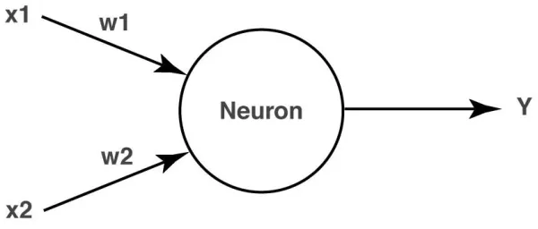
information, called input, going into their bodies (Gurney, 1997). All of the inputs from connections with other neurons are added up according to a summation algorithm. As in their biological counterparts, the signal will continue to the next neuron if the added input exceeds a threshold; otherwise, it will not be transmitted. The strength or weakness of the connections between neurons is controlled by “weights.” If the weight is high, it will ensure that the neuron gets activated, i.e. the signal gets transmitted. If, on the other hand, the weight is small or negative, it will work to inhibit the neuron and keep the signal from being transmitted.

3.3.1 Single Layer Networks: The McCulloch-Pitts Neuron, the Perceptron, and the Adaline

The first artificial model representing a biological neuron was proposed by

Figure 3-3: The Artificial Neuron - the McCulloch-Pitts Neuron.

The neuron uses the transfer function I= Σ(wixi), where I is the net weighted input, wi is

the weight vector, and xi the input vector. Theoretically, it is very simple. The neuron computes the weighted sum of the inputs and compares it to the threshold value of the neuron (Caudill and Butler, 1992). If the net input is greater than or equal to the threshold, the neuron outputs +1; otherwise, the output is -1.

In 1958, Frank Rosenblatt provided the first procedure that allowed a network to learn a task. Known as the perceptron, the algorithm of this network allowed weight values to be updated, and thus training was achieved (Caudill and Butler, 1992). The equation used was as follows:

wnew = wold + (βyx) [3-5]

where,

β= +1, if perceptron output is correct, -1 otherwise

A simple perceptron can be represented by a single neuron that applies a step function to the net weighted sum of its inputs. The input pattern belongs to one class or the other depending on whether the output is 0 or 1.

Even though the perceptron has a training algorithm allowing weight modification to reduce the number of misclassifications, it does not always perform efficiently. A more robust procedure is needed to improve separation between samples of different classes. The separation is improved by minimizing the mean square error (MSE) or the sum squared error (SSE) of the network (Mehrotra et al., 1997).

In 1960, Bernard Widrow and Ted Hoff came up with a network that used the minimum error technique. This network, known as the Adaline (ADAptive LINear Element), was the first example of a practical supervised training algorithm (Caudill and Butler, 1992). It accomplished classification by modifying the weights to reduce the MSE at every pattern presentation, even when the sample was correctly classified (Mehrotra et al., 1997). Having a bipolar output, the Adeline outputs +1 when the net weighed sum is greater than 0 and -1 when it is less than or equal to 0. Generally a class is assigned to each of the output values, i.e. +1 represents class A, -1 class B (Caudill and Butler, 1992). The transfer function used is that designed by McCulloch and Pitts: I = Σ(wixi). If the net input I is greater than zero, the Adeline outputs +1 (input pattern

response is correct. The next pattern is then presented. When the delta rule is applied to a pattern, the weights of the previous pattern(s) are checked to verify that the response is still correct. If the response to the second pattern is still correct, no weight change is done, and the third pattern is presented. If, on the other hand, the response is incorrect, the delta rule is applied again until the correct response is reached. Each time all patterns are presented to the network is called an iteration or an epoch (Braspenning et al., 1995). It often takes many iterations to modify the weights, decrease the network’s error, and correctly train the network. It is this process of weight adjustment plus the rechecking of previous patterns that makes the algorithm of the Adaline more complex.

3.3.2 The Delta Rule

The delta rule, also called the Widrow-Hoff or the least mean square (LMS) method, functions by adjusting corrections for errors. The rule is often applied to associated pairs of patterns, the input and corresponding output pattern. In an Adeline with multiple inputs, the error associated with the network is measured in terms of the MSE. Let xi = (i0, i1, ... , in) be the input vector and yi the desired output of the neuron.

The net input to the neuron is the transfer function Ii = Σj(wjxj), where w = (wo, ... , wn) is

the weight vector. The squared error is found by squaring the difference between the desired output, yi, and the actual output, Ii:

2 ) (

2 1

i i I

y

E= − [3-6]

) ( ) ( _i k i i k I w I y w E ₋ ∂ ∂ − = ∂ ∂

∑

=( ) ( ( _{j i}))

k i

i w x

w I y i k i i k x I y w E , ) ( − = ∂ ∂ [3-7]

To minimize the error, a gradient descent rule is applied to equation 3-5:

x x x w y

w_k = ( _i −

∑

∆ η

j i i k y I x

w = ( − )

∆ η [3-8]

The delta rule algorithm, which is used to update the weights and decrease the network’s error, is often described by the following equation (Khanna, 1990):

x w=ηδ

∆ [3-9]

Where: η = learning constant (between 0 and 1) δ = error of the network

x = input vector w = weight vector

3.3.3 Multi-layered Networks and the Backpropagation Algorithm

The networks previously described, the perceptron and the Adeline, are single-neuron networks. Thus, their computational ability is limited to solving only problems that are linearly separable. In other words, the networks can properly solve only

problems in which a line exists that separates all the samples of one class from the other (Mehrotra et al., 1997). In order to solve real world problems, i.e. not linearly separable, a multiple layer network is needed. The most common network combines several

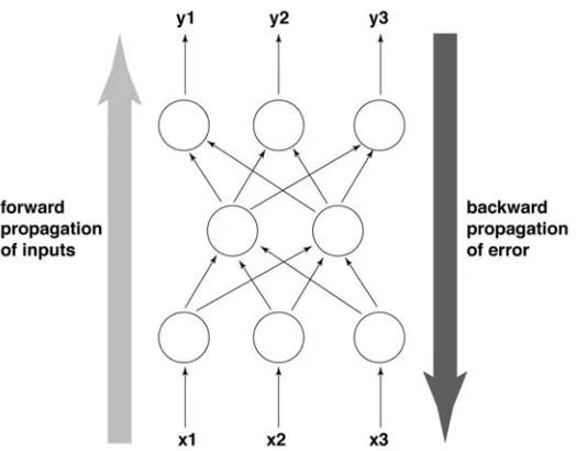
In the 1970s and 1980s, a backpropagation (BP) training algorithm was developed for a multi-layered network, one capable of solving problems that were not linearly separable. It makes ANNs very powerful and successful for various applications such as image compression, speech and pattern recognition, and recognition of written zip codes, among others. Even though alternative learning algorithms have emerged since the creation of BP, it is still the most widely used learning algorithm in the realm of neural networks (Orr and Muller, 1998). A backpropagation network modifies the LMS rule, or delta rule, used by the Adeline to make it appropriate for a multilayered network (Caudill and Butler, 1992). The resulting algorithm is called the generalized delta rule.

Figure 3-4: The Two-Phase Procedure for a Backpropagation Neural Network.

Generally, a backpropagation network consists of at least three fully

interconnected layers (input, hidden, and output). Every neuron in a layer has an output connected to every neuron in the following layer. For example, in a typical three layer network, such as in Figure 3-4, the neurons in the input layer (x) connect only to those of the hidden layer, which in turn connect only to those in the output layer (y). There is no limit to the number of hidden layers in a BP network, but research has shown that a single hidden layer is adequate to solve many problems (Braspenning et al., 1995). Information from the input layer is propagated through the neural network layer by layer (Gurney, 1997).

Hidden units need activation functions in order to introduce non-linearity to the neural network (Principe et al., 2000). It is this non-linearity that makes multi-layer networks powerful. Without it, the networks would just be plain perceptrons, which have no hidden units. For a backpropagation network, the activation function must be

is often used as well. The tanh function produces both positive and negative values and tends to train faster than functions that produce only positive values, such as the logistic function.

For the output units, activation functions suited to the distribution of the target values are the best choice. For binary target values (0/1), the logistic function is widely used (Jordan, 1995). If the target values do not have a known bounded range, it is better to use an unbounded activation function, such as the identity function.

Hidden and output units usually use a “bias” or “threshold” term to compute the net input to the unit (Principe et al., 2000). The term “bias” refers to a “bias unit,” a neuron whose input is a constant value of one. Generally, every hidden and output unit has its own bias term though they are not usually shown graphically in a neural network’s architecture. Even though the input of the bias is constant, the weights of each bias unit are not, hence bias terms can learn just like the other neurons. The term “threshold” refers to a constant value of -1. Regardless of which term is used, adding or subtracting from the neuron’s net input has no effect on the network’s performance.

Backpropagation neurons are similar to the McCulloch-Pitts neuron but differ in the activation function (Caudill and Butler, 1992). As in their primitive neuron, the net

weighted input is computed using I =

∑

0 0.2 0.4 0.6 0.8 1 1.2

-5 -4 -3 -2 -1 0 1 2 3 4 5

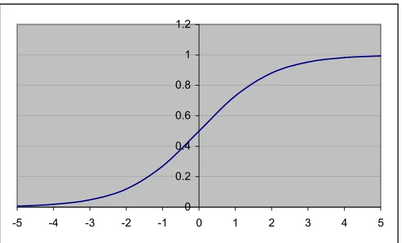
Figure 3-5: The Graph of the Logistic Sigmoid Function.

The most popular is the logistic sigmoid activation function (Figure 3-5), which is defined as: I e I f ₋ + = 1 1 )

( [3-10]

The derivative of this function is:

      + − + = + − + = + = −₋ −_{− − −} ) 1 ( 1 1 ) 1 ( 1 ) 1 ( ) 1 ) 1 (( ) 1 ( ) ( 2

2 I I I

I I I e e e e e e dI I df

(

)

) ( ) ( I f I f dI I

df _{= −}

[3-11]

3.3.4 The Generalized Delta Rule

As previously stated, backpropagation networks use a training algorithm called the generalized delta rule, which is also based on gradient descent (Caudill and Butler, 1992). The change in a given weight is defined as

) (I f w_ij =ηδ

∆ [3-12]

Where: δ = error for neuron

η = learning constant (normally between 0 and 1) f(I) = input to the neuron

Two main differences exist between this algorithm and that of the Adeline (Caudill and Butler, 1992). First, the net input is modified by the logistic sigmoid function (equation 3-10). The second difference deals with the computation of the error, E. In the Adeline, the error is generated by subtracting the actual output from the desired output. In a backpropagation network, the derivative of the activation function is multiplied by this difference. For the middle layer, the procedure gets more complex due to the lack of a desired output value (Khanna, 1990). The error of the output layer is passed back to the middle layer and weighted by the same connections used in the forward pass (Caudill and Butler, 1992). In other words, the error for the neurons in the hidden layer is determined in terms of the neurons and the weights in the following layer (Khanna, 1990). The net error in each neuron in the middle layer is multiplied by the derivative of the activation function. Thus, mathematically, the error computation in the network is defined as:

Output layer:

(

)

' −

=

δ [3-13]

(

)

3.3.5 Momentum

A well-trained neural network is very efficient in comparing unknown samples with respect to a number of known references (Hodgins, 1997). Training a BP neural network, however, can take many iterations to reduce the error to an acceptable value. In order to reduce the lengthy training period, a momentum term is often added to the generalized delta rule. Sometimes a BP network does not train in a reasonable period of time, and the total error stops decreasing therefore stalling at an unacceptable value. The network is stuck in a local minimum. The addition of a momentum term to the algorithm helps to avoid this problem. The weight change with momentum is defined as:

previous ij

ij f I w

w = + ∆

∆ ηδ ( ) α [3-15]

Where: η = learning constant

δ = error of neurons in proceeding layer f(I) = input to neuron

α = momentum constant (usually between 0 and 1)

4 Materials and Methods

The North Carolina State University electronic nose (NC State e-nose) was designed and built under the direction of Dr. H. Troy Nagle in the Department of Electrical and Computer Engineering. The sensor array of the e-nose contains 16 tin metal oxide sensors. A mass flow controller is used to modify the air flow (l/min) through the array of sensors. Table 4-1 shows the cross sensitivities of the tin metal oxide sensors of the electronic nose (Dodd et al., 2000).

Table 4-1: Cross Sensitivities of the Sensors Used in the NC State E-nose. Sensor

Number

Sensor Type Part

(manufacture)

Cross Sensitivities

0 Ethanol AAS14 (Capteur) Oxidizable Solvents and vapors 1 Iso Propyl Alcohol AAS20 (Capteur) Oxidizable Solvents and vapors 2 Hydrogen Sulfide GS05 (Capteur) Amonia, Propane, CO

3 Toluene AAS25 (Capteur) Oxidizable Solvents and vapors 4 Ammonia GS06 (Capteur) Hydrogen Sulfide, Propane, CO 5 Carbon Monoxide GL07 (Capteur)

6 Propane CTS03 (Capteur) Oxidizable Solvents and vapors 7 Hydrogen CTS23 (Capteur) Oxidizable Solvents and vapors 8 Chlorine LGS09 (Capteur) Ozone, NOx

9 Nitrogen Dioxide LGS10 (Capteur) Hydrogen Sulfide, Ozone, Chlorine 10 Butane CTS04 (Capteur) Oxidizable Solvents and vapors 11 Sulphur Dioxide GS22 (Capteur) CO, Some Solvents

12 Solvent Vapors TGS2620 (Figaro) 13 Combustible Gases TGS2610 (Figaro) 14 Methane TGS2611 (Figaro) 15 Air Contaminants TGS2600 (Figaro)

74 pyrroles, 70 ketones, 44 phenols, 31 hydrocarbons, 30 esters, 28 aldehydes, 28

oxazoles, 27 thiazoles, 26 thiophenes, 21 amines, 20 acids, 19 alcohols, 13 pyridines, and 13 thiols/sulfides (Bartlett et al., 1997). The overlap of sensitivities increases the range of organic volatile compounds detected by the e-nose; hence, fewer sensors are needed to detect an aroma.

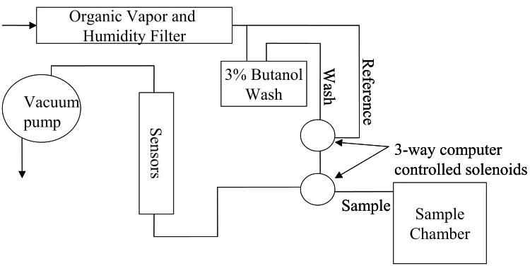
Operation of the NC State e-nose is controlled via a LabVIEW® data acquisition program. Figure 4-1 shows the flow diagram of the e-nose (Dodd et al., 2000).

Organic Vapor and Humidity Filter Sample Chamber 3% Butanol Wash S ens or s Vacuum pump W as h R ef er enc e Sample 3-way computer controlled solenoids Organic Vapor and

Humidity Filter Sample Chamber 3% Butanol Wash S ens or s Vacuum pump W as h R ef er enc e Sample 3-way computer controlled solenoids

Figure 4-1: Flow Diagram of the NC State E-nose.

The four-phase sampling procedure consists of the following steps:

2) Reference #1: Ambient air is pumped through the charcoal filter (resulting in odor-free and dry air) at a flow rate of 5 l/min for a duration of 210 seconds. Sensor resistance returns to the starting baseline (reference).

3) Reference #2: This step is the same as in step 2 (reference #1) except the flow rate is 2 l/min for 30 seconds. This second flow rate matches the flow rate used in the data acquisition step to ensure that sensor response is caused by an odor instead of a change in the air flow.

4) Data acquisition: Headspace sample gases are pumped through the sensor array at a flow rate of 2 l/min for a duration of 60 seconds. The sensor response (in volts) is saved at a rate of 1 Hz, giving a total of 60 points/sensor, for every sample.

4.2 Preparation of SkipJack Tuna Samples

A single SkipJack tuna (Katsuwonus pelamis) was cut into four 3.8 cm steaks. A #7 cork borer was used to gather twelve 1.3 cm x 3.1 cm (diameter x length) cylindrical samples from the light meat of each of three steaks. In order to have equal dimensions among samples, they were individually trimmed on both sides to achieve the 3.1 cm length. The samples were then numbered one to thirty-six and randomly assigned to one of three treatments: raw, heated to 55°C, and heated to 85°C. Each of the samples in the

(one to thirty-six) and stored in a freezer (0ºC). The day prior to e-nose analysis, the samples were placed in the refrigerator overnight. This was done so the samples would generate a headspace in the vials. On the day of analysis, each sample was taken out of the refrigerator, placed in a beaker of ice, and analyzed by the electronic nose. After e-nose analysis, the sample was placed back in the refrigerator, and a new sample was taken out for analysis. This was done until all the samples were analyzed. All the samples were then placed back in the freezer. This procedure was repeated on three different days, a week apart. For each day of e-nose analysis, a different randomization was chosen to select the order in which the samples were analyzed.

4.3 Data Analysis

The three days of e-nose analysis were combined into one data set to form a database of tuna samples. The combined data set was then analyzed taking the sample’s treatment into consideration (1 = raw, 2 = heated to 55°C, and 3 = heated to 85°C).

E-nose data were compressed with a moving bell integral from 60 to 4 points per sensor1. PCA and LDA were used for feature extraction. The compressed data were randomly divided into a training set (60%) and a testing set (40%). PCA and LDA features from the training set and testing sets were used to classify data using LS and KNN. Data from the bell integral were used to train a feed-forward ANN with a backpropagation

algorithm. The network was trained until every data point fed into the network was correctly classified. The testing set was used to determine a percentage of correctly classified samples. The data analysis procedure was done 10 consecutive times with

5 Results and Discussion

The resistance value of sensor #6 (Table 4-1) remained at a constant value for every sample and day of e-nose analysis; therefore, it was removed prior to performing data analysis. This sensor is designed to detect propane, an explosive gas; therefore, it is unlikely that the removal of this sensor affected the results of this study. The following sections explain the results of the feature extraction methods (thesis objective #2) and the classification algorithms (thesis objective #3).

5.1 Feature Extraction Methods

Figures 5-1 and 5-2 are the graphical representation of LDA and PCA,

Figure 5-1: LDA Projections for Treatment Classification.

Figure 5-2 exhibits the results of PCA. The amounts of variation of the original data set contained by principal component 1 (PC1) and principal component 2 (PC2) were 61.93% and 35.31%, respectively. Hence, 97.24% of the total variation in the original data set is contained in the first two principal components. PCA was not able to separate the individual samples into groups representing the sample’s treatment. Since PCA does not take the class assignment into consideration, the resulting classification is independent of the class given to identify each sample’s treatment. Based on the

Figure 5-2: PCA Projections for Treatment Classification.

Figure 5-3: PCA Graph Showing Discrimination Among Days of E-nose Analysis.

Several factors can contribute to the group associations represented in the PCA graphs. The samples were analyzed on three separate days, a week apart. Between days of e-nose analysis, the samples were frozen and thawed. Thawing and freezing of the samples can contribute to a change in the sample’s chemical composition, hence affecting the aroma of the sample as well. The PCA graph could be describing the differences in aroma after each freezing and thawing process.

sensor’s output to a desirable level. Due to the variability of each sensor, i.e. sensitivity to the change in resistance, it is improbable that all the sensors started at the same baseline for every day of e-nose analysis. The sample associations seen in Figures 5-2 and 5-3 could be due to PCA discriminating between samples based on sensor drift instead of sample treatment.

If sensor drift is, in fact, the reason why PCA sorts by day, it is possible that it affects LDA as well. Figure 5-1 shows that LDA discriminates among samples based on treatment, hence the sensor drift does not affect it as much as in PCA. The reason for this is probably the fact that LDA is a supervised method of feature extraction. In other words, it knows what treatment each sample belongs to and works to maximize the difference among treatments while minimizing the difference among samples in the same treatment.

Figure 5-4: Second (PC2) and Third (PC3) Principal Components.

Based on these graphs (Figures 5-4 and 5-5), it can be seen that PC2 is more important for classification purposes than PC3. This is verified in Figure 5-2 as well. The first PC is only able to divide the classification “plane” into a left and a right zone. It discriminates between the cluster on the left and the two on the right. It is unable,

however, to discriminate between the two right-hand clusters. On the other hand, PC2 permits separation among the three clusters of data, which represent each day of e-nose analysis. Hence, it can be concluded that, regardless of the amount of total variance in the original data set, PC2 is more important in classification than PC1 even though classification is not based on sample treatment.

A 3-D graph was also created by adding the third principal component. The graph, however, did not show discrimination among treatments either. This suggests that either the remaining principal components that contain only 0.86% of the total variation are needed to discriminate among treatments (a highly unlikely scenario) or that PCA is not able to sort tuna samples based on cooking treatment at all.

5.2 Data Classification Algorithms

Table 5-1: Comparison of Classification Percentages, Mean (Standard Deviation).

Feature

Extraction PCA LDA None

Classifier KNN LS KNN LS ANN

% Correct 36.4 (3.7) 47.1 (4.0) 53.3 (6.4) 50.2 (5.2) 43.3 (5.7) Paired t-tests were used to reveal statistical significance among methods of data classification. The following data classification methods were not found to be

significantly different (two-tail P > 0.05): PCA+LS and LDA+LS; LDA+KNN and LDA+LS; and PCA+LS and ANN. The remaining comparisons (PCA+KNN and ANN; LDA+KNN and ANN; and LDA+LS and ANN) were found to be significantly different.

Figures 5-6 and 5-7 show the data points of LDA and PCA, respectively, used to classify the testing set with LS and KNN. The samples in the testing set are marked with an asterisk (*); the remaining samples (the dark clusters) correspond to the training set.

In LDA, the training set is used to find the eigenvalues (aip in Equation 2-11) which are then used to find the discriminant functions (the model). The values of the testing set (Xp in Equation 2-11) are then passed through the model with the eigenvalues created by the training set. The new discriminant functions represent the data in the testing set.

Figure 5-6: LDA Training and Testing Sets Based on Treatment. Numbers with an Asterisk (*) Represent Test Data.

The LDA classification percentages of the data set can be verified by observing the graph of the training and testing LDA sets (Figure 5-6). The number of DFs returned by LDA is the minimum of the number of variables (60 in this study) and the number of classes minus one (3-1=2). Hence, the number of DFs in this model is only two, those represented by the axes of the graph in Figure 5-6. Because both LS and KNN

Verification of classification percentages is not as easily estimated with PCA because it returns many projections. The graphs only show data represented by two principal components, but more can be used to classify data even if they cannot be displayed graphically. Usually, four principal components account for about 99.0-99.5% of the total variation in the data set. The classification methods, KNN and LS, used all of the PCs to find a percentage of correctly classified samples. A problem can occur when a PC contains information that is not important for classification of the data. The results of Figures 5-2 and 5-4 reveal that, in this study, PC2 has a bigger role in classification than PC1. It is possible that using PC1 could lead to a sample being incorrectly classified and, thus, lowering the classification percentage. This, however, does not rule out that the low classification percentages can be also due to the fact that PCA was not able to

discriminate among treatments.

Even though PCA discriminated based on day of e-nose analysis and was not a suitable method for feature extraction in this study, it is a powerful method. This can be verified by comparing Figures 5-2 and 5-7. In Figure 5-2, PCA is done on the whole data set. In Figure 5-7, however, PCA is only done on the training set (60% of the data set). The eigenvalues (aij in Equation 2-1) are found by using the training set. The testing set values (Xp) are then multiplied by their corresponding eigenvalues to create the PCs of the testing set. The samples of the testing set, marked with an asterisk in Figure 5-7, were placed in the same position on the PCA graph as those seen in Figure 5-2. This shows that PCA is not greatly affected by a reduction in the number of samples in the training set, from 100% to 60% of the original data, and that PCA is able to accurately predict unseen samples using the reduced data set.

LDA, on the other hand, is affected by the size of the training set. Figure 5-1 represents LDA on the whole data set. Figure 5-6 represents the training (60% of the data set) and testing samples (40% of the data set) of LDA. The DFs are found in the same manner as the PCs in PCA. The training set is used to find the eigenvalues of the DFs. The values of the testing set are multiplied by these eigenvalues to derive the DFs that represent the testing set. The samples of the testing set in Figure 5-6 were not placed in the same or similar positions as those seen in Figure 5-1. The clear separation among treatments is not seen in Figure 5-6. Hence, the size of the training set affects LDA performance and accuracy of predicting unseen samples.

output unit was chosen to be linear in order to decrease computational time in training the network. Funahashi (1989) and Hornik et al. (1989) have shown that ANNs with linear output units can approximate any continuous function by increasing the size of the hidden layer. Hence, using a linear instead of a sigmoid activation function does not affect the network’s classification ability. The 60 input nodes represent the data from the bell integral (4 points/sensor x 15 sensors = 60).

Table 5-2: Topology and Parameters Used in the ANN.

Type of network: feed-forward Learning algorithm: backpropagation

Number of inputs-hidden-output neurons: 60 – 30 – 1 Hidden layer activation function: sigmoid

Output layer activation function: linear Learning rate: 0.003

Momentum: 1.00

To avoid saturation in the sigmoid hidden units and to speed up training time, the data from the bell integral were scaled. Each column vector in the training set, i.e. each input into the network, was normalized by subtracting the mean and dividing by the standard deviation of that column. Training was continued until all the samples in the training set were within ± 0.1 of their target values. After training the ANN, the testing set was used on a plain feed-forward ANN without learning, i.e. no backpropagation. The samples were assigned to a class label based on the classification criteria of Table 5-3. Any sample generating a network output less than 0.5 or greater than 5-3.5 was

Table 5-3: Classification Criteria for the Testing Data of the ANN.

Network’s Ouput Class Assignment 0.50 – 1.49 1

1.50 – 2.49 2 2.50 – 3.49 3

The ANN was not the best classification method for e-nose data. It achieved a better classification percentage than KNN with PCA but worse than the rest of the classification methods (Table 5-1). Two main factors that can affect the network’s performance are:

1. Overfitting – During training, the network also learns the noise in the training set, which hinders its ability to predict unknown samples in the testing set. The higher the number of weights in the network, relative to the number of cases in the training set, the more overfitting amplifies the noise. 2. Underfitting – In this case, the network does not learn effectively, which

results in excessive bias in the outputs. The network is unable to accurately predict the samples in the testing set, therefore creating a low percentage of correctly classified samples.

Based on the output generated by the ANN, it is worth noting an interesting observation. A greater number of samples in treatment 2 (55°C) were misclassified as

belonging to treatment 3 (85°C). There is a simple solution that might explain this

occurrence. The temperatures for these two treatments represent two major peaks of protein denaturation. The measurements for treatment 2 contain information about the physiological and chemical changes of the samples at 55°C. It is possible that the

samples in the 85°C treatment also contain this information, as well as other information

representing the changes that occur between the 55°C and 85°C temperatures. Hence, in

addition to extra information, the samples in treatment 3 could also contain the

information already displayed in the samples of treatment 2. This could have caused the ANN to assign some samples in treatment 2 to treatment 3.

Due to the possible overlap of information between treatment 2 and treatment 3, the samples in the 55°C treatment were taken out of the data set. The data analysis

(described in Section 4.3) was repeated for just the raw and heated to 85°C samples.

Table 5-4 compares the percentages of correctly classified samples in the three methods used to classify e-nose data.

Table 5-4:Correct Classification Percentages of the Samples in Treatments 1 and 3.

Feature Extraction PCA LDA None

Classifiers KNN LS LS / KNN ANN

Mean 50.0 62.1 73.9 61.1

Standard Deviation 7.9 10.5 9.4 9.3

statistically different (P < 0.05) except those in bold. LS using LDA features and LDA+KNN had the highest data classification percentages. LDA+KNN and LDA+LS achieved the same classification percentages, which was also the highest value. They were the same because LDA, for this case, returned only one DF. KNN computes all the distances from the test samples to the rest of the samples and assigns the sample to the group with the shortest distance via a majority vote. The use of one DF (1-D space) makes KNN behave like LS, hence the classification percentages are exactly the same.

Theoretically, an e-nose would be used to classify an unknown based on an existing database of samples. As opposed to some multivariate analysis techniques that come with commercial e-noses, these databases do not come with the e-noses. Hence, the database needs to be built from scratch. E-nose data gathering can be very time consuming and may yield only a small data set per day of analysis. A small data set will cause unsatisfactory results in both feature extraction, classification algorithms, and ANN generalization. If data gathering expands over several days, there is concern that sensor drift could affect the outcome of the data analysis.

Another disadvantage of ANN is the inability to determine how the network is making its decision; hence, it is hard to determine which data are important and useful for classification. The use of the bell integral data, for example, can be affecting the

These features have then been used as inputs into the ANN, thus reducing the time spent in trial-and-error to find the optimal parameters needed to achieve a good network

generalization. If, as in this study, the features do not correctly represent the original data set or represent another relationship in the samples (as in PCA – Figures 2 through 5-5), it is unlikely that the ANN will achieve desirable results.

Even though many researchers have reported that BP ANNs outperform some statistical pattern recognition techniques, there is still no formula to find the optimal solution. Some researchers have also found the use of ANNs to be less than satisfactory. Gorman and Sejnowski (1988) used a 60-24-2 neural network to classify sonar signals bounced off a metal cylinder. Their test set on the NN generated an average error rate of 10.8%. Rippley (1994) repeated the experiment using a 60/40 training and testing set, respectively, to train and test a neural network. Out of five neural network runs, the average test set error was 41.4 out of 84 or 49.3%.

6 Conclusion and Recommendations

This study used an electronic nose to classify tuna samples processed at three different levels: raw, heated to 55ºC, and heated to 85ºC. LDA proved to be a better feature extraction method than PCA. PCA sorted the data according to day of e-nose analysis and not sample treatment. In PCA, not all of the components were important for data classification. The second principal component proved to be more important in the classification of the e-nose data by day of e-nose analysis than the first principal

component. In spite of the fact that PCA was not able to discriminate among the treatments, it showed promise because it modeled the data better than LDA. In this study, LDA+KNN and LDA+LS proved to be better methods than ANN for data classification. The results from this study indicate that the use of a backpropagation ANN to classify data correctly is limited. It could be possible that the network overfitted the data because of the small training set. Overall, the ANN with backpropagation performed better than PCA with KNN but worse than PCA with LS and any method using LDA.

Based on the results gathered from this research, some recommendations can be made for future studies:

a) It would be beneficial to test the following changes on the sampling procedure of the NC State e-nose to see if the time of the sampling procedure can be reduced: i) The reference cycle, used after the 3% n-butanol wash, was 270 s, which

decreasing the time spent in the reference cycle, hence more samples could be analyzed by the e-nose during a fixed time period.

ii) Currently, the duration in the sampling phase is set to 60 s. This duration might or might not be suitable for the samples in this study. According to Kermani et al. (1999) “long exposure of the sensors to some odorants can cause irreversible changes in the baseline resistance and, thus, should be avoided.” Reducing this time to 30 s, for example, would potentially avoid the irreversible baseline sensor changes and also allow more samples to be analyzed by the e-nose in a fixed time period.

b) Currently, many of the parameters in a neural network are found by trial and error. It would be beneficial to find a way to determine these parameters experimentally. Kermani et al. (1999) used genetic algorithms, based on

Darwin’s survival of the fittest theory, to find the network parameters that would enhance the network’s performance and generalization. Even though it requires more computational ability, it could be beneficial in the long run.

c) The results of this research reveal that the first principal component might not be important for classification purposes. It would be beneficial to use different PCs to determine which ones contain the information necessary to classify a sample. d) PCA proved to be a powerful method to correctly predict unseen examples. It is

e) Several modifications could be made to the backpropagation algorithm to attempt to achieve a better generalization:

i) Weight decay – used for a large-sized ANN. A decay constant is applied to the weights to drive all the unnecessary weights to zero during adaptation. Therefore, only the important weights are kept, thus decreasing the number of free parameters in the network.

ii) Early stopping – training is stopped at a certain point. After a certain point in the training, the SSE of the training set continues to decrease but the SSE of the testing set increases. This method stops training when the testing set SSE is lowest.

iii) Using a different learning constant for each weight – similar to weight decay. Theoretically, this method helps the weights achieve their optimum value. f) Other ANN algorithms can be used instead of the standard backpropagation, such