Quantitative Analysis of Variability and Uncertainty in On-Road and Non-Road Mobile Source Emission Factors

(1)

ABSTRACT

BAMMI, SACHIN. Quantitative Analysis of Variability and Uncertainty in On-Road

and Non-Road Mobile Source Emission Factors. (Under the direction of Dr. H

Christopher Frey.)

The goal of this research is to demonstrate a methodology for quantifying variability and uncertainty in mobile source emissions. Emission factors and emission estimates are subject to both variability and uncertainty. Variability in emissions deals with real differences in emissions among multiple emission sources at any given time or over time for any individual emission source. Variability is the heterogeneity of values of a quantity with respect time space or across a population. Uncertainty in emissions on the other hand implies the lack of knowledge regarding the true va lue of emissions. In this research variability and uncertainty are treated separately since their sources are different and as such they affect the decision making process in a different way. For example, sources of variability in mobile source emissions include: vehicle make; ambient temperature; vehicle model; fuel used; vehicle age; and/or driving behavior. Sources of uncertainty may include: small sample sizes; lack of precision and/or accuracy in measurements; non-representativeness; or lack of data.

(2)

This methodology is demonstrated for emission factors for three categories: (1) Onroad mobile source exhaust air toxic emissions (2) nonroad lawn and garden

equipment emissions and (3) nonroad construction farm and industrial equipment emissions. For the first category a database of vehicular exhaust emissions developed by the California Air Resources Board (CARB) was used. For the second and third

categories emission factor databases were developed by reviewing reports and/or

technical papers from U.S. Environmental Protection Agency (EPA), Southwest Research Institute (SwRI), CARB and Society of Automotive Engineers (SAE).

The main results regarding the demonstrated methodology and related statistical analysis in this research include: (1) emission factor groupings were determined

(3)

(4)

Biography

(5)

Acknowledgments

The size of the “people sets” that I want to thank unlike the size of the data sets that I analyzed for this research is large. Though there is a lot of variability amongst the people in the people sets I want to thank, there is no uncertainty in the fact that without their co-operation and help this work would not have been possible.

First I want to thank my family (kat, golu, billu and bhujang) for supporting me and being there for me all along. If not for them, I would have been a very different me and I am sure I wo uldn’t have liked that.

I am grateful to Dr. H. C. Frey for his invaluable guidance throughout this effort. I thank Mr. James Warila of U.S. EPA’s Office of Mobile Sources in Ann Arbor, MI for his assistance and recommendations regarding data sources and Mr. Charles T. Hare, Director of Department of Emissions Research, Southwest Research Institute for kindly providing me with emission test reports. I also want to thank my committee members Dr. John W. Baugh Jr. and Dr. E. Downey Brill, Jr. for their inputs in this effort.

(6)

Padmanabh (pseud) Pai (pai). They helped me feel at home away from home and have been/are like my family in the US.

I thank Sujay Kumar (SV) and Arvind Srinivasan (Cool Dude) for being great friends on whom I could always depend on. CE537 and my Distributed GA project in the summer of 2000 would have been a lot tougher if it had not been for their help in

debugging my java programs.

I thank people in my research group: Matt Pickett, Alper Unal, Song Li, Sumeet Patil, Junyu Zheng (Allan), Chi Xie (Dennis), Yuchao Zhao (Maggie), Minshing Li (Michael) and Amr Abdel- Aziz. Working along with these folks was a great learning experience. I will always cherish the long discussions I had with Sudeep, Matt and Alper on Life, Religion among other things that are best left unsaid. I greatly appreciate the help I got from Alper in understanding the is sues related to statistical data analysis that came up while I was working on the project. My appreciation for American English grew after I learned the myriad words in American Slang from Matt.

(7)

Table of Contents

List of Tables ...viii

List of Figures ...xi

1.0 INTRODUCTION ... 1

1.1 Probabilistic Analysis of Emission Inventories ...4

1.2 Methodology for Characterizing Variability and Uncertainty...5

1.2.1 General Approach... 6

1.2.2 Visualization of Data ... 6

1.2.3 Empirical Cumulative Distribution Functions ... 7

1.2.4 Bootstrap Methodology ... 11

1.3 Overview of Thesis ...12

2.0 AIR TOXIC EMISSIONS FROM ON-ROAD MOBILE SOURCES ... 14

2.1 Exhaust Toxics Emissions Modeling Methodology ...15

2.1.1 Previous EPA Estimates ... 15

2.1.2 Complex Model for Reformulated Gasoline... 17

2.1.3 Treatment of Normal and High Emitters: “Toxic-TOG Curves” .... 18

2.2 Methodology Used to Analyze CARB Data ...25

2.2.1 Finding Most Useful Measure of Emissions... 26

2.2.2 Characterization of Uncertainty... 34

2.2.3 Development of Probabilistic Toxic-TOG Curves ... 34

2.2.4 Effect of Fuel Used ... 44

2.3 Uncertainty in Toxic Emissions as Percent of TOG...46

2.4 Summary...57

3.0 LAWN AND GARDEN ENGINE EMISSIONS ... 59

3.1 A Review of Technologies...59

3.1.1 Application vs. Power Rating ... 61

3.1.2 Two-Stroke vs. Four-Stroke... 62

3.1.3 Overhead Valve (OHV) Design vs. Side Valve (LHV) Design ... 62

3.1.4 Handheld vs. Non-Handheld... 63

3.2 Steady State Test Procedures for the Measurement of Exhaust Emissions from Small Utility Engines...63

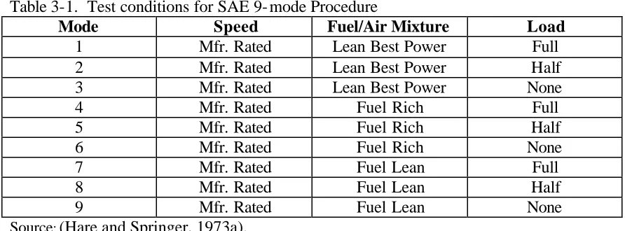
3.2.1 SAE 9-Mode Procedure ... 64

3.2.2 Modified EMA 13-Mode ... 65

3.2.3 6-Mode Method... 66

3.2.4 C6M Method ... 66

3.2.5 SAE J1088... 68

3.2.6 CARB J1088 Procedure ... 82

3.2.7 SAE J1088 “A” Procedure ... 83

3.2.8 SAE J1088 “C” (90:10 & 70:30) Procedure ... 84

3.2.9 Lawn Mower Cycle... 84

3.2.10 Generator Set Cycle ... 85

3.3 Data Analysis ...85

3.3.1 Reproducing Reported Emission Factors... 86

3.3.2 Comparing the Test Cycles... 92

(8)

3.3.4 Grouping the Test Data ... 97

3.4 Analysis of Variability and Uncertainty ...105

3.4.1 Quantification of Inter-Engine Variability and Uncertainty in Mean of Emissions ... 106

3.4.2 Results of Quantitative Analysis of Variability and Uncertainty in L&G Engine Emission Factors ... 107

4.0 CONSTRUCTION, FARM AND INDUSTRIAL ENGINE EMISSIONS... 116

4.1 Emission Test Procedures ...117

4.1.1 CARB 13-Mode Procedure ... 118

4.1.2 21-Mode Procedure... 119

4.1.5 S-1, S-2 and S-3 Test Procedures ... 122

4.1.6 Agricultural Tractor Cycle, Backhoe Loader Cycle and Crawler Dozer Cycle... 124

4.2 Reproducing Reported Emission Factors...124

4.3 Comparing the Test Cycles...130

4.3.1 Comparison of 21-Mode and 13-Mode Test Procedures ... 132

4.3.3 Comparison of 21-Mode and S-1, S-2 and S-3 Test Procedures ... 141

4.3.5 Comparison of 8-mode and Agricultural Tractor, Crawler Dozer and Backhoe Loader Test Procedures ... 143

4.4 Summary of the Database ...148

4.5 Grouping the Test Data ...152

4.5.1 Categorizing Emission Factors By Fuel ... 153

4.5.2 Categorizing Diesel Engine Emission Factors By Technology... 153

4.5.3 Categorizing 4-stroke Diesel Engine Emission Factors By Engine Type ... 154

4.5.4 Categorizing Diesel Engine Emission Factors By Engine Age ... 154

4.5.5 Categorizing Diesel Emission Factors By Engine Size ... 155

4.6 Analysis of Variability and Uncertainty ...158

4.6.1 Quantification of Inter-Engine Variability in Emissions ... 159

4.6.2 Characterization of Uncertainty in CFI Engine Emission Factors ... 159

4.6.3 Results of the Uncertainty Analysis... 164

5.0 CONCLUSIONS, RECOMMENDATIONS AND FUTURE WORK ... 167

6.0 REFERENCES ... 174

7.0 APPENDIX A: Additional Figures for Chapter 2 ... 186

8.0 APPENDIX B: Additional Figures for Chapter 3... 204

9.0 APPENDIX C: Additional Figures for Chapter 4... 214

(9)

Database for 4-stroke Gasoline Fueled Engines ...226

12.0 APPENDIX F: Construction, Farm and Industrial Engine Emission Factor Database ... 229

13.0 APPENDIX G: Unavailable Data Sources ... 236

Data Sources From Engine Manufactures Association (EMA)...236

Data Sources From Outdoor Power Equipment Institute (OPEI)...238

(10)

List of Tables

Table 1-1. Contribution of Mobile Sources in the total National Emissions of

air pollutants: VOCs, NOx, CO and HAPs. ...1 Table 1-2 Expressions for Log-Likelihood Functions for Data Belonging to

Various Probability Distribution Models. ...11 Table 2-1. Exhaust Toxics Fractions as a % of TOG Emissions used by EPA

in 1993 MVRATS ...16 Table 2-2. Example Data for development of Benzene Toxic-TOG curves. ...19 Table 2-3. Summary of the Variability Analysis Done for all the Five

Pollutants Using Data Collected by the Federal Test Procedure. ...26 Table 2-4. Summary of the Variability Analysis Done for all the Five

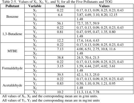
Pollutants Using Data Collected by the Unified Cycle Procedure. ...27 Table 2-5. Values of X1, X2, Y1, and Y2 for all the Five Pollutants and TOG...37 Table 2-6. Summary of Probabilistic Distributions used to Develop

Toxic-TOG curves...38 Table 2-7. Variability Analysis of Y1 and Y2 Values for All the Five

Pollutants...38 Table 2-8. Summary of the Variability Analysis of Predicted Air Toxic

Emissions ...44 Table 2-9. Results of Comparison of Percent of TOG Using the Fuels RFG

and UnL Based Upon t-Tests for the Difference of Two Means at a

5% Level of Significance. ...45 Table 2-10. Results of Comparison of Percent of TOG Using the Fuels RFG

and Indolene Based Upon t-Tests for the Difference of Two Means

at a 5% Level of Significance ...45 Table 2-11. Results of Comparison of Percent of TOG Using the Fuels

Indolene and UnL Based Upon t-Tests for the Difference of Two

Means at a 5% Level of Significance...46 Table 2-12. Summary of Fitted Distributions for all Five Pollutants: (High and

Normal Emitters Both)...51 Table 2-13. Summary of Fitted Distributions for all Five Pollutants: (Only

High Emitters)...51 Table 2-14. Summary of Fitted Distributions for all Five Pollutants: (Only

Normal Emitters)...51 Table 2-15. Mean and the 95% Confidence Intervals (CI) of the Mean of the

Fitted Distributions for Five Pollutants (as %TOG) (High and

Normal Emitters both): CASE 1 ...53 Table 2-16. Mean and the 95% Confidence Intervals (CI) of the Mean of the

Fitted Distributions for Five Pollutants (as %TOG) (High

Emitters): CASE 2 ...53 Table 2-17. Mean and the 95% Confidence Intervals (CI) of the Mean of the

(11)

Table 2-18. Summary of Variability in Emission Factor Data for High and

Normal Emitters for all the Five Pollutants in units of % of TOG. ...56

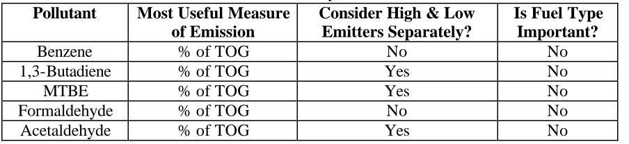
Table 2-19. Final recommendations of the study...58

Table 3-1. Test conditions for SAE 9- mode Procedure ...65

Table 3-2. Test conditions for “Modified EMA 13- mode” Procedure...66

Table 3-3. C6M Test Cycle Description ...67

Table 3-4. 16 Engine Operating Modes of the SAE J1088 Procedure ...77

Table 3-5. Utility Engine Applications – Typical Operating Modes Compared to the SAE J1088 Procedure ...78

Table 3-6. Engine Operating/Performance Parameters to be Reported in the SAE J1088 Procedure ...79

Table 3-7. Units of Measured Initial Molar Concentrations ...79

Table 3-8. Proposed CARBJ1088 Modes and Weighting Factors ...83

Table 3-9. Comparison of Selected L&G Equipment Test Cycles Based on the Number of Modes and Type of Engine Load ...93

Table 3-10. Summary of the L&G Engine Emission Factor Database ...96

Table 3-11. Results of Comparison of Non-Handheld versus Handheld Emissions Data Based Upon t-Tests for the Difference of Two Means at a 5% Level of Significance...98

Table 3-12. Results of Comparison of 2-Stroke versus 4-Stroke Engine Emissions Data, and of OHV versus LHV 4-Stroke Engines, Based Upon t-Tests for the Difference of Two Means at a 5% Level of Significance...98

Table 3-13. Results of Comparison of Size Ranges for 4-Stroke and for 2-Stroke Engines Based Upon t-Tests for the Difference in Mean Emissions at a 5% Level of Significance...104

Table 3-14. Results of the Uncertainty Analysis of Mean NOx and THC Emission Rates for 2-Stroke and 4-Stroke Lawn and Garden Engines for Three Emission Factor Units (g/gal, g/h, and g/hp-h) ...112

Table 3-15. Comparison of the Mean of Data Sets with the Mean of the Fitted Distribution for All the Emission Factor Categories ...115

Table 4-1. Test conditions for 13-Mode and 21-Mode Test Procedures...120

Table 4-2. Test Conditions for 23-Mode Procedure...121

Table 4-3. Test Conditions for 8-Mode Procedure...122

Table 4-4. Test Conditions for S-1, S-2 and S-3 Test Procedures ...123

Table 4-5. Comparison of Steady-State CFI Equipment Test Procedures Based on the Number of Modes and Type of Engine Load...131

Table 4-6. Summary of the Results of the Inter-Cycle Comparisons ...138

Table 4-7. Summary of the L&G Engine Emission Factor Database ...149

Table 4-8. Summary of the Information About the Type of Tests done on each Engine in the Database...150 Table 4-9. Results of Comparison of Diesel versus Gasoline Engines, Old

(12)

-Tests for the Difference of Two Means at a 5% Level of

Significance...158 Table 4-10. Results of the Uncertainty Analysis of Mean NOx and THC

Emission Rates for Diesel and Gasoline fueled CFI Engines in

units of g/hp-h. ...162 Table 4-11. Summary of the Comparison Between the Mean of the Data Sets

(13)

List of Figures

Figure 1-1. Empirical Distribution Function for NOx Emission Factor of

2-Stroke Lawn & Garden Engines in Units of g/hp- hr. ...8

Figure 2-1. An Example of Benzene-TOG Curve ...22

Figure 2-2. Corrected Example Benzene-TOG Curve ...25

Figure 2-3. Variability in Benzene Emissions (mg/mi) Using FTP Cycle ...29

Figure 2-4. Variability in Benzene Emissions (Percent of TOG) Using FTP Cycle ...29

Figure 2-5. Variability in Benzene Emissions (mg/mi) Using Unified Cycle...29

Figure 2-6. Variability in Benzene Emissions (Percent of TOG) Using Unified Cycle ...30

Figure 2-7. Scatter Plot of Benzene Concentration vs TOG for FTP Cycle ...30

Figure 2-8. Scatter Plot of Benzene Concentration vs THC for FTP Cycle ...30

Figure 2-9. Scatter Plot of Benzene Concentration vs TOG for UC Cycle ...32

Figure 2-10. Scatter Plot of Benzene Concentrtion vs THC for UC Cycle ...33

Figure 2-11. Scatter Plot of Benzene Concentration as Percent of TOG vs. TOG (g/mi) for the FTP cycle...33

Figure 2-12. Scatter Plot of Benzene Concentration as Percent of TOG vs. TOG (g/mi) for the Unified cycle ...33

Figure 2-13. Fitted Lognormal Distribution to the Values of Y1 for Benzene ...37

Figure 2-14. Probabilistic Benzene Toxic-TOG Curves ...39

Figure 2-15. Probabilistic 1,3-Butadiene Toxic-TOG Curves...39

Figure 2-16. Probabilistic MTBE Toxic-TOG Curves ...39

Figure 2-17. Probabilistic Formaldehyde Toxic-TOG Curves ...40

Figure 2-18. Probabilistic Acetaldehyde Toxic-TOG Curves ...40

Figure 2-19. Variability in Predicted Target Fuel Benzene Emissions for Base Fuel TOG = 1 g/mi...41

Figure 2-20. Variability in Predicted Target Fuel 1,3- Butadiene Emissions for Base Fuel TOG = 1 g/mi ...42

Figure 2-21. Variability in Predicted Target Fuel MTBE Emissions for Base Fuel TOG = 1 g/mi...42

Figure 2-22. Variability in Predicted Target Fuel Formaldehyde Emissions for Base Fuel TOG = 1 g/mi ...42

Figure 2-23. Variability in Predicted Target Fuel Acetaldehyde Emissions for Base Fuel TOG = 1 g/mi ...43

Figure 2-24. Bootstrap Simulation Results for MTBE Emissions as % of TOG for Both Normal and High Emitters (All Fuels). ...50

Figure 2-25. Bootstrap Simulation Results for MTBE Emissions as % of TOG for High Emitters only (All Fuels). ...50

Figure 2-26. Bootstrap Simulation Results for Benzene Emissions as % of TOG for Normal Emitters only (All Fuels)...50

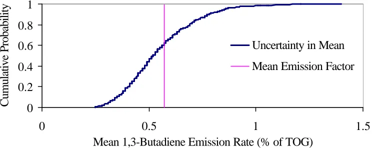
Figure 2-27. Uncertainty in 1,3-Butadiene Mean Emission Factor (% of TOG) ...54

(14)

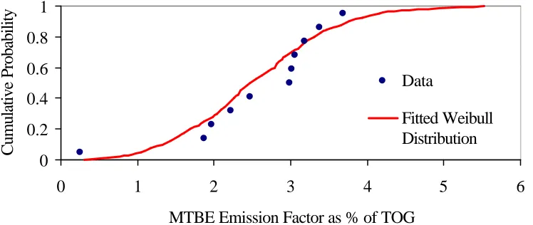
Figure 2-29. Fitted Weibull Distribution for MTBE Emission Factor Data for

Normal Emitters Only in Units of % of TOG. ...55 Figure 3-1. Engine Setup for Emissions Tests...70 Figure 3-2. Exhaust Gas Analysis System...74 Figure 3-3. Scatter Plot of THC (g/hp- h) Emission Factors for 4-Stroke L&G

Engines Versus the Size of the Engine (Rated Horsepower)...102 Figure 3-4. Scatter Plot of THC (g/gallon) Emission Factors for 2-Stroke L&G

Engines Versus the Size of the Engine (Rated Horsepower)...102 Figure 3-5. Fitted Lognormal Distribution and Bootstrap Simulation Results

for 2-Stroke L&G Engine NOx Emission Data in Units of g/hp-hr. ...108 Figure 3-6. Fitted Lognormal Distribution and Bootstrap Simulation Results

for 2-Stroke L&G Engine THC Emission Data in Units of g/hp-hr. ...110 Figure 3-7. Fitted Lognormal Distribution and Bootstrap Simulation Results

for 4-Stroke L&G Engine NOx Emission Data in Units of g/hp-hr. ...110 Figure 3-8. Fitted Lognormal Distribution and Bootstrap Simulation Results

for 4-Stroke L&G Engine THC Emission Data in Units of g/hp-hr. ...110 Figure 4-1. Variation of Speed and Torque During the Agricultural Tractor

Cycle. Source: (EPA, 2001 c) ...125 Figure 4-2. Variation of Speed and Torque during the Crawler Dozer Cycle.

Source: (EPA, 2001 c) ...125 Figure 4-3. Variation of Speed and Torque during the Backhoe Loader Cycle.

Source: (EPA, 2001 c) ...125 Figure 4-4. Comparison Between THC Emission Factors Measured with the

21-Mode Test and Those Developed from 13-Mode Test Data ...133 Figure 4-5.. Comparison Between NOx Emission Factors Measured with the

21-Mode Test and Those Developed from 13-Mode Test Data. ...133 Figure 4-6. Comparison Between THC Emission Factors Developed from

13-Mode Test Data Extracted from 21-13-Mode Test and those Measured

with 21-Mode Test. ...136 Figure 4-7. Comparison Between NOx Emission Factors Developed from

13-Mode Test Data Extracted from 21-13-Mode Test and those Measured

with 21-Mode Test. ...136 Figure 4-8. Comparison Between THC Emission Factors Developed from

13-Mode Test Data Extracted from 21-13-Mode Test and those

Developed from 13-Mode Test Data. ...137 Figure 4-9. Comparison Between NOx Emission Factors Developed from

13-Mode Test Data Extracted from 21-13-Mode Test and those

Developed from 13-Mode Test Data. ...137 Figure 4-10. Comparison Between THC Emission Factors Measured with the

21-Mode Test and those Developed from 8-Mode Test Data

Extracted from 21-Mode Test Data. ...140 Figure 4-11. Comparison Between NOx Emission Factors Measured with the

21-Mode Test and those Developed from 8-Mode Test Data

(15)

Figure 4-13. Comparison Between Corrected NOx Emission Factors Measured with the 13-Mode Test and those Measured With the 23-Mode Test

Data ...144

Figure 4-14. Scatter Plot to Compare the THC Emission Factors Developed Using the 8-Mode Steady State Cycle and the Agricultural Tractor Transient Cycle. ...146

Figure 4-15. Scatter Plot to Compare the THC Emission Factors Developed Using the 8-Mode Steady State Cycle and the Crawler Dozer Transient Cycle. ...146

Figure 4-16. Scatter Plot to Compare the THC Emission Factors Developed Using the 8-Mode Steady State Cycle and the Backhoe Loader Transient Cycle. ...146

Figure 4-17. Scatter Plot to Compare the NOx Emission Factors Developed Using the 8-Mode Steady State Cycle and the Backhoe Loader Transient Cycle. ...147

Figure 4-18. Scatter Plot of THC (g/hp- hr) Emission Factors for 4-Stroke Engines Versus the Size of the Engine (Rated Horsepower)...157

Figure 4-19. Scatter Plot of NOx (g/hp-hr) Emission Factors for 4-Stroke Engines Versus the Size of the Engine (Rated Horsepower)...157

Figure 4-20. Fitted Weibull Distribution and Bootstrap Simulation Results for CFI Gasoline Engine THC Emission Data in Units of g/hp-hr ...161

Figure 4-21. Fitted Weibull Distribution and Bootstrap Simulation Results for 2-Stroke CFI Diesel Engine NOx Emission Data in Units of g/hp- hr...161

Figure 4-22. Fitted Lognormal Distribution and Bootstrap Simulation Results for 4-Stroke Diesel CFI Engine NOx Emission Data in Units of g/gallon...163

Figure 23. Fitted Gamma Distribution and Bootstrap Simulation Results for 4-Stroke Diesel CFI Engine THC Emission Data in Units of g/gallon...164

Figure 7-1. Variability in 1,3-Butadiene Emissions (mg/mi) Using FTP Cycle ...186

Figure 7-2. Variability in 1,3-Butadiene Emissions (% of TOG) Using FTP Cycle ...186

Figure 7-3 Variability in 1,3-Butadiene Emissions (mg/mi) Using UC Cycle ...186

Figure 7-4 Variability in 1,3-Butadiene Emissions (% of TOG) Using UC Cycle ...187

Figure 7-5 Variability in MTBE Emissions (mg/mi) Using FTP Cycle...187

Figure 7-6 Variability in MTBE Emissions (% of TOG) Using FTP Cycle ...187

Figure 7-7 Variability in MTBE Emissions (mg/mi) Using UC Cycle ...188

Figure 7-8 Variability in MTBE Emissions (% of TOG) Using UC Cycle ...188

Figure 7-9 Variability in Formaldehyde Emissions (mg/mi) Using FTP Cycle...188

Figure 7-10 Variability in Formaldehyde Emissions (%of TOG) Using FTP Cycle ...189

Figure 7-11 Variability in Formaldehyde Emissions (mg/mi) Using UC Cycle ...189

Figure 7-12 Variability in Formaldehyde Emissions (%of TOG) Using UC Cycle ...189

(16)

Figure 7-14 Variability in Acetaldehyde Emissions (%of TOG) Using FTP

Cycle ...190

Figure 7-15 Variability in Acetaldehyde Emissions (mg/mi) Using UC Cycle ...190

Figure 7-16 Variability in Acetaldehyde Emissions (% of TOG) Using UC Cycle ...191

Figure 7-17 Scatter Plot of 1,3-Butadiene (mg/mi) vs. TOG (g/mi) Using FTP Cycle ...191

Figure 7-18 Scatter Plot of 1,3-Butadiene (mg/mi) vs. THC (g/mi) Using FTP Cycle ...191

Figure 7-19 Scatter Plot of 1,3-Butadiene (mg/mi) vs. TOG (g/mi) Using UC Cycle ...192

Figure 7-20 Scatter Plot of 1,3-Butadiene (mg/mi) vs. THC (g/mi) Using UC Cycle ...192

Figure 7-21 Scatter Plot of MTBE (mg/mi) vs. TOG (g/mi) Using FTP Cycle ...192

Figure 7-22 Scatter Plot of MTBE (mg/mi) vs. THC (g/mi) Using FTP Cycle ...193

Figure 7-23 Scatter Plot of MTBE (mg/mi) vs. TOG (g/mi) Using UC Cycle ...193

Figure 7-24 Scatter Plot of MTBE (mg/mi) vs. THC (g/mi) Using UC Cycle ...193

Figure 7-25 Scatter Plot of Formaldehyde (mg/mi) vs. TOG (g/mi) Using FTP Cycle ...194

Figure 7-26 Scatter Plot of Formaldehyde (mg/mi) vs. THC (g/mi) Using FTP Cycle ...194

Figure 7-27 Scatter Plot of Formaldehyde (mg/mi) vs. TOG (g/mi) Using UC Cycle ...194

Figure 7-28 Scatter Plot of Formaldehyde (mg/mi) vs. THC (g/mi) Using UC Cycle ...195

Figure 7-29 Scatter Plot of Acetaldehyde (mg/mi) vs. TOG (g/mi) Using FTP Cycle ...195

Figure 7-30 Scatter Plot of Acetaldehyde (mg/mi) vs. THC (g/mi) Using FTP Cycle ...195

Figure 7-31 Scatter Plot of Acetaldehyde (mg/mi) vs. TOG (g/mi) Using UC Cycle ...196

Figure 7-32 Scatter Plot of Acetaldehyde (mg/mi) vs. THC (g/mi) Using UC Cycle ...196

Figure 7-33. Scatter Plot of 1,3-Butadiene Concentration as Percent of TOG vs. TOG (g/mi) for FTP Cycle ...196

Figure 7-34. Scatter Plot of 1,3-Butadiene Concentration as Percent of TOG vs. TOG (g/mi) for the Unified Cycle. ...197

Figure 7-35. Scatter Plot of MTBE Concentration as Percent of TOG vs. TOG (g/mi) for FTP Cycle...197

Figure 7-36. Scatter Plot of MTBE Concentration as Percent of TOG vs. TOG (g/mi) for the Unified Cycle...197

(17)

Figure 7-39. Scatter Plot of Acetaldehyde Concentration as Percent of TOG vs.

TOG (g/mi) for FTP Cycle ...198 Figure 7-40. Scatter Plot of Acetaldehyde Concentration as Percent of TOG vs.

TOG (g/mi) for the Unified Cycle. ...199 Figure 7-41 Bootstrap Simulation Results for Benzene Emissions as % of TOG

for Both Normal and High Emitters...199 Figure 7-42 Bootstrap Simulation Results for 1,3-Butadiene Emissions as % of

TOG for Both Normal and High Emitters. ...199 Figure 7-43 Bootstrap Simulation Results for Formaldehyde Emissions as % of

TOG for Both Normal and High Emitters. ...200 Figure 7-44 Bootstrap Simulation Results for Acetaldehyde Emissions as % of

TOG for Both Normal and High Emitters. ...200 Figure 7-45 Bootstrap Simulation Results for Benzene Emissions as % of TOG

for High Emitters Only. ...200 Figure 7-46 Bootstrap Simulation Results for 1,3-Butadiene Emissions as % of

TOG for High Emitters Only. ...201 Figure 7-47 Bootstrap Simulation Results for Formaldehyde Emissions as % of

TOG for High Emitters Only. ...201 Figure 7-48 Bootstrap Simulation Results for Acetaldehyde Emissions as % of

TOG for High Emitters Only. ...201 Figure 7-49 Bootstrap Simulation Results for Benzene Emissions as % of TOG

for Low Emitters Only. ...202 Figure 7-50 Bootstrap Simulation Results for 1,3-Butadiene Emissions as % of

TOG for Low Emitters Only. ...202 Figure 7-51. Bootstrap Simulation Results for Formaldehyde Emissions as % of

TOG for Low Emitters Only. ...202 Figure 7-52 Bootstrap Simulation Results for Acetaldehyde Emissions as % of

TOG for Low Emitters Only. ...203 Figure 8-1. Scatter Plot of THC (g/h) Emission Factors for 4-Stroke L&G

Engines Versus the Size of the Engine (Rated Horsepower)...204 Figure 8-2. Scatter Plot of THC (g/gallon) Emission Factors for 4-Stroke L&G

Engines Versus the Size of the Engine (Rated Horsepower)...204 Figure 8-3. Scatter Plot of NOx (g/h) Emission Factors for 4-Stroke L&G

Engines Versus the Size of the Engine (Rated Horsepower)...204 Figure 8-4. Scatter Plot of NOx (g/hp-h) Emission Factors for 4-Stroke L&G

Engines Versus the Size of the Engine (Rated Horsepower)...205 Figure 8-5. Scatter Plot of NOx (g/gallon) Emission Factors for 4-Stroke L&G

Engines Versus the Size of the Engine (Rated Horsepower)...205 Figure 8-6. Scatter Plot of THC (g/h) Emission Factors for 2-Stroke L&G

Engines Versus the Size of the Engine (Rated Horsepower)...205 Figure 8-7. Scatter Plot of THC (g/hp- h) Emission Factors for 2-Stroke L&G

Engines Versus the Size of the Engine (Rated Horsepower)...206 Figure 8-8. Scatter Plot of NOx (g/h) Emission Factors for 2-Stroke L&G

Engines Versus the Size of the Engine (Rated Horsepower)...206 Figure 8-9. Scatter Plot of NOx (g/hp-h) Emission Factors for 2-Stroke L&G

(18)

Figure 8-10. Scatter Plot of NOx (g/gallon) Emission Factors for 2-Stroke L&G

Engines Versus the Size of the Engine (Rated Horsepower)...207 Figure 8-11. Bootstrap Simulation Results for 2-stroke L&G Gasoline Engine

NOx Emission Data in Units of g/gallon. ...207 Figure 8-12. Bootstrap Simulation Results for 2-stroke L&G Gasoline Engine

NOx Emission Data in Units of g/hr. ...207 Figure 8-13. Bootstrap Simulation Results for 2-stroke L&G Gasoline Engine

THC Emission Data in Units of g/gal. ...208 Figure 8-14. Bootstrap Simulation Results for 2-stroke L&G Gasoline Engine

THC Emission Data in Units of g/hr...208 Figure 8-15. Bootstrap Simulation Results for 4-stroke L&G Gasoline Engine

NOx Emission Data in Units of g/gal. ...208 Figure 8-16. Bootstrap Simulation Results for 4-stroke L&G Gasoline Engine

NOx Emission Data in Units of g/hr. ...209 Figure 8-17. Bootstrap Simulation Results for 4-stroke L&G Gasoline Engine

THC Emission Data in Units of g/gal. ...209 Figure 8-18. Bootstrap Simulation Results for 4-stroke L&G Gasoline Engine

THC Emission Data in Units of g/hr...209 Figure 8-19. Bootstrap Simulation Results for 4-stroke L&G Gasoline Engine

NOx Emission Data in Units of g/gal (Size ≥ 8 hp). ...210 Figure 8-20. Bootstrap Simulation Results for 4-stroke L&G Gasoline Engine

NOx Emission Data in Units of g/hr (Size ≥ 8 hp)...210 Figure 8-21. Bootstrap Simulation Results for 4-stroke L&G Gasoline Engine

NOx Emission Data in Units of g/hp- hr (Size ≥ 8 hp). ...210 Figure 8-22. Bootstrap Simulation Results for 4-stroke L&G Gasoline Engine

NOx Emission Data in Units of g/gal (Size < 8 hp). ...211 Figure 8-23. Bootstrap Simulation Results for 4-stroke L&G Gasoline Engine

NOx Emission Data in Units of g/hr (Size < 8 hp)...211 Figure 8-24. Bootstrap Simulation Results for 4-stroke L&G Gasoline Engine

NOx Emission Data in Units of g/hp- hr (Size < 8 hp). ...211 Figure 8-25. Bootstrap Simulation Results for 4-stroke L&G Gasoline Engine

THC Emission Data in Units of g/gal (Size ≥ 8 hp). ...212 Figure 8-26. Bootstrap Simulation Results for 4-stroke L&G Gasoline Engine

THC Emission Data in Units of g/hr (Size ≥ 8 hp). ...212 Figure 8-27. Bootstrap Simulation Results for 4-stroke L&G Gasoline Engine

THC Emission Data in Units of g/hp-hr (Size ≥ 8 hp)...212 Figure 8-28. Bootstrap Simulation Results for 4-stroke L&G Gasoline Engine

THC Emission Data in Units of g/gal (Size < 8 hp). ...213 Figure 8-29. Bootstrap Simulation Results for 4-stroke L&G Gasoline Engine

THC Emission Data in Units of g/hr (Size < 8 hp). ...213 Figure 8-30. Bootstrap Simulation Results for 4-stroke L&G Gasoline Engine

THC Emission Data in Units of g/hp-hr (Size < 8 hp). ...213 Figure 9-1. Scatter Plot to Compare the THC Emission Factors Developed

(19)

Figure 9-2. Scatter Plot to Compare the THC Emission Factors Developed Using the Backhoe Loader Cycle and the Agricultural Tractor

Transient Cycles...214 Figure 9-3. Scatter Plot to Compare the THC Emission Factors Developed

Using the Crawler Dozer Cycle and the Backhoe Loader Transient

Cycles...214 Figure 9-4. Scatter Plot to Compare the NOx Emission Factors Developed

Using the Crawler Dozer Cycle and the Agricultural Tractor

Transient Cycles...215 Figure 9-5. Scatter Plot to Compare the NOx Emission Factors Developed

Using the Backhoe Loader Cycle and the Agricultural Tractor

Using the 8-Mode Steady State Cycle and the Agricultural Tractor

Using the 8-Mode Steady State Cycle and the Crawler Dozer

Using the Crawler Do zer Cycle and the Agricultural Tractor

Using the Backhoe Loader Cycle and the Agricultural Tractor

Using the 8-Mode Steady State Cycle and the Agricultural Tractor

Using the 8-Mode Steady State Cycle and the Crawler Dozer

Transient Cycles...218 Figure 9-14. Scatter Plot of THC (g/hr) Emission factors for 4-Stroke Engines

Versus the Size of the Engine (Rated Horsepower)...218 Figure 9-15. Scatter Plot of NOx (g/hr) Emission Factors for 4-Stroke Engines

Versus the Size of the Engine (Rated Horsepower)...218 Figure 9-16. Scatter Plot of THC (g/gallon) Emission Factors for 4-Stroke

Engines Versus the Size of the Engine (Rated Horsepower)...219 Figure 9-17. Scatter Plot of NOx (g/gallon) Emission Factors for 4-Stroke

Engines Versus the Size of the Engine (Rated Horsepower)...219 Figure 9-18. Bootstrap Simulation Results for CFI Gasoline Engine NOx

(20)

Figure 9-19. Bootstrap Simulation Results for 2-stroke CFI Diesel Engine THC

Emission Data in Units of g/hp-hr ...220 Figure 9-20. Bootstrap Simulation Results for 4-Stroke Diesel CFI Engine NOx

Emission Data in Units of g/hr ...220 Figure 9-21. Bootstrap Simulation Results for 4-Stroke Diesel CFI Engine NOx

Emission Data in Units of g/hp-hr ...220 Figure 9-22. Bootstrap Simulation Results for 4-Stroke Diesel CFI Engine THC

Emission Data in Units of g/hr ...221 Figure 9-23. Bootstrap Simulation Results for 4-Stroke Diesel CFI Engine THC

(21)

1.0 INTRODUCTION

Mobile sources, both onroad and nonroad, are majors contributors to the total national emissions of Volatile Organic Compounds (VOCs), Nitrogen Oxides (NOx) and Carbon Monoxide (CO) (EPA, 2000 b). They also contribute significantly to the total emissions of the Hazardous Air Pollutants (HAPs) (EPA, 2001 b). Table 1-1 shows the contribution of the mobile sources as a percentage of the total national emissions. The percentages shown for HAPs are 1996 figures while those of the others are 1998 numbers. It is clear that mobile sources contribute substantially to the total national emissions of several key pollutants.

Table 1-1. Contribution of Mobile Sources in the total Nationa l Emissions of air pollutants: VOCs, NOx, CO and HAPs.

Emissions of Mobile Source

VOC a NOx a CO a HAP b

On-Road Contribution (%) 29 31 57 30

Non-Road Contribution (%) 14 22 22 20

Total Contribution (%) 43 53 79 50

a

Values for year of 1998, (EPA, 2000 b). b

Values for the year of 1996, (EPA, 2001 b).

Section 112(k) of Title III of the Clean Air Act Amendments of 1990 requires EPA to develop a strategy for controlling emissions of 188 listed air toxics or HAPs. Section 112 focuses on stationary and area sources. Other sections of the act in particular, Section 202(1) contains two specific requirements for motor vehicles (Sierra Research, 1999):

(22)

• EPA was to promulgate regulations containing requirements to control air toxic emissions from motor vehicles and motor vehicle fuels by May 15th, 1995.

Presently EPA is concentrating on 33 air toxics that present the greatest threat to public health in largest number of urban areas under a national scale air toxics assessment program (EPA, 2001 a). Mobile sources are one of the major contributors to air toxic emissions. They account for 50 percent (30% highway vehicles or onroad mobile sources + 20% nonroad mobile sources) of the total 1996 annual air toxic emissions of 4.6

million tons, for all the 188 listed air toxics. Of the annual 1996 emissions of the 33 air toxics (1.1 million tons/year) the mobile sources account for 51 percent (29% highway vehicles or onroad mobile sources + 22% nonroad mobile sources) (EPA, 2001 b). Acetaldehyde, Benzene, 1,3-butadiene and formaldehyde figure in this list of top 33 HAPs mentioned above.

The 1990 Clean Air Act Amendments specifically directed the U.S.

(23)

primarily used in lawn and garden applications. While diesel fueled nonroad compression ignition (CI) engines contribute to about 20 percent NOx emissions from mobile sources. These engines are primarily used in construction, farm and industrial applications (EPA, 2000 a). Currently, neither uncertainty nor variability is properly quantified in these HAP and nonroad emission factors and emission inventories.

Emission factors and emissions estimates are subject both to variability and uncertainty. Variability refers to real differences in emissions among multiple emission sources at any given time or over time for any individual emission source. Variability in emissions can be attributed to variation in: fuel or feedstock composition; ambient temperature; process design; process maintenance; and/or process operation. Uncertainty refers to lack of knowledge regarding the true value of emissions. Sources of uncertainty include: small sample sizes; lack of precision and/or accuracy in measurements; non-representativeness; or lack of data (Bammi and Frey, 2001).

Emission Inventories (EIs) are an important part of environmental decision making. They are used for temporal emissions trend characterization, emissions budgeting for regulatory and compliance purposes and in air quality models for estimating ambient air quality. Non-quantified errors and biases in the EIs can lead to erroneous conclusions regarding emissions trends, apportionment of emissions, compliance, and the relationship between emissions and the ambient pollutant

(24)

recommended that efforts be conducted to quantify uncertainties in mobile source emissions (NRC 2000).In this work, a quantitative approach to the characterization of variability and uncertainty is presented and used as an important means to convey the quality of estimates to analysts and decision makers. This work focuses on the

application of quantitative analysis of variability and uncertainty to different case studies for mobile source emission categories.

1.1 Probabilistic Analysis of Emission Inventories

(25)

EPA, the National Academy of Sciences (NAS), and others recognize the important role of probabilistic analysis (NRC 1994; NRC 2000) In March 1997, EPA issued “Guiding Principles for Monte Carlo Analysis” (EPA 1997). The policy supports “good scientific practices” in quantifying variability and uncertainty. Therefore it is critically important that research be undertaken in the development and application of probabilistic methods. An overview of probabilistic ana lysis methods is given by Cullen and Frey (1999). The recent NRC recommendations regarding uncertainty analysis for mobile sources also motivate this work (NRC 2000). There have been some efforts to quantify uncertainty in mobile sources, focused on highway vehicles (Kini and Frey, 1997; Pollack et al., 1999; Frey et al., 1999). In addition, there has been work to quantify uncertainties in emissions of stationary point and area sources (Frey et al., 1999; Frey and Rhodes, 1996; Rhodes and Frey, 1997; Frey and Li, 2001). In this thesis, a methodology for simultaneous characterization of both variability and uncertainty is presented, with applications to on-road and non-road mobile emission sources.

1.2 Methodology for Characterizing Variability and Uncertainty

(26)

1.2.1 Gene ral Approach

The following are the major steps of the general approach described by Frey et al. (1999) to characterize variability and uncertainty in emission factors and emission

inventories. It was applied where applicable to the data sets analyzed in this work. 1 Compilation and evaluation of database for emission and activity factors. 2 Developing empirical cumulative distribution functions (CDF) for each

emission and activity factor to visualize the data. To test for dependencies between pairs of activity and emission factors. Scatter plots are also developed.

3 Representing variability in activity and emission factor data by fitting, evaluating and selecting from alternative parametric probability distribution models.

4 Characterizing uncertainty in the distributions for variability.

5 Estimation of uncertainty in emissions from a population of emission sources by propagating uncertainty and variability in activity and emissions factors.

1.2.2 Visualization of Data

(27)

variables. All the quantities considered in this study are assumed to be continuous random variables.

1.2.3 Empirical Cumulative Distribution Functions

Distributional data may often be summarized using empirical cumulative distribution functions (Cullen and Frey, 1999). These functions provide a relationship between fractiles (or percentiles) and quantiles. A quantile is a value of a random variable associated with a given fractile. To get an indication of the dispersion of the distribution we may, for example, be interested in knowing the range enclosed by the 0.01 and 0.99 fractiles.

1.2.3.1 Plotting Position

To estimate the fractile or percentile from data requires rank ordering of the data. The methods used for estimating the percentile of an empirically observed data point are called “plotting positions.” The plotting position is an estimate of the cumulative

probability of a data point. As described by Cullen and Frey (1999), Harter (1984) provides an overview of the various types of plotting positions. A commonly used plotting position, proposed by Hazen (1914), is used in this study.

Fx(xi) = Pr(X < xi) = (i – 0.5)/n (1-1)

for i = 1,2,…,n and x1 < x2 < …< xn

where,

i = Rank of the data point when the data set is arranged in an ascending order

(28)

x1 < x2 < …< xn are data points in the rank ordered set

Pr(X < xi) = Cumulative probability of obtaining a data point whose value is less

than or equal to xi

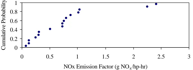
As an example, empirical distribution function for 16 data points of the NOx emission factor of 2-Stroke Lawn and Garden (L & G) engines in units of g/hp- hr, based on Equation (1.1), is shown in Figure 1.1. The data used in this example is discussed in detail in Chapter 3. The figure illustrates that the central tendency of the emission factors is toward a value of approximately 0.73 g/hp- hr, as reflected by the median (50th

percentile). The 95 percent probability range indicates the dispersion of the emission factors range from approximately 0.08 g/hp-hr to 2.5 g/hp-hr. In this case the distribution is positively skewed, with a heavier tail of values to the right.

Figure 1-1. Empirical Distribution Function for NOx Emission Factor of 2-Stroke Lawn & Garden Engines in Units of g/hp-hr.

1.2.3.2 Parametric Probability Distribution Models

A probability distribution model is a description of the probabilities of all possible sets of outcomes in a range space (Cullen and Frey, 1999). One class of probability

0 0.2 0.4 0.6 0.8 1

0 0.5 1 1.5 2 2.5 3

NOx Emission Factor (g NOx/hp-hr)

(29)

models are described by their parameters. The advantage of using them is that data sets containing potentially large numbers of samples can be described by a probability model that is defined by typically one to four parameters. Two of the most common approaches for estimating the parameters of a distribution are the method of matching moments (MoMM) and maximum likelihood estimation (MLE). MoMM is based upon matching moments or central moments of a fitted parametric distribution (like mean, variance) to the moments or central moments of the data set. Usually MoMM estimators are easy to calculate. For example Hahn and Shapiro (1967) present convenient solutions for MoMM parameter estimates for Normal, Lognormal, Gamma and Weibull distributions. The maximum likelihood estimation approach involves selecting values of distribution parameters to define a distribution that is most likely to yield the observed data set (Cohen and Whitten, 1988). For independent samples, a likelihood function is defined as the product of the Probability Density Function (PDF) evaluated at each of the sample values. For a continuous random variable for which independent samples have been obtained, the likelihood function is:

L( θ1, θ2,…,θk) = ( | 1, 2,...., ) 1

k n

i

x

f θ θ θ

∏

=

, (1-2)

where,

θ1, θ2,…,θk = Parameters of the parametric probability distribution

k = number of parameters for the parametric probability distribution model

(30)

The value of k usually is either two (for a two-parameter distribution) or three (for a three-parameter distribution). Standard techniques of calculus are used sometimes to determine the values of the parameters that maximize the likelihood function. However, usually log transformations of the likelihood functions (referred to as log likelihood functions) are used because of the convenience involved with working with them. For cases when an analytical solution is not readily available, the MLE parameters can be found using numerical techniques such as Newton-Raphson method or non-linear programming optimization (Bharvirkar, 1999).

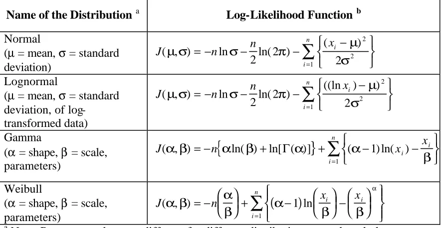
Table 1-2 presents the log- likelihood functions for estimating the parameters of Normal, Lognormal, Gamma and Weibull distributions (Bharvirkar, 1999). The number of data points is n and each data point is represented as xi, where i takes the values 1

through n.

The maximum likelihood estimates do not always yield minimum variance or unbiased estimates for small sample sizes. However, for larger sample sizes the

(31)

Table 1-2 Expressions for Log-Likelihood Functions for Data Belonging to Various Probability Distribution Models.

Name of the Distribution a Log-Likelihood Function b Normal

(µ = mean, σ = standard deviation)

J n n xi

i n

( , )µ σ lnσ ln( π) ( µ)

σ = − − −  −     =

∑

2 2 2

2

2 1

Lognormal

(µ = mean, σ = standard deviation, of

log-transformed data)

J n n xi

i n

( , )µ σ lnσ ln( π) ((ln ) µ)

σ = − − −  −     =

∑

2 2 2

2

2 1

Gamma

(α = shape, β = scale, parameters)

}

{

J n x_i xi

i n

( , )α β α βln( ) ln[ ( )]α (α ) ln( )

β = − + + _ − −     =

∑

Γ 1 1 Weibull

(α = shape, β = scale, parameters)

(

)

J n xi xi

i n

( , )α β α ln

β α β β α = −    _ + −    _ −_ _         =

∑

1 1 a

Note: Parameter values are different for different distributions even though the same symbol has been used to represent their parameters.

b

Source: Masters Thesis (Chapter 2) of Ranjit Bharvirkar (Bharvirkar, 1999).

1.2.4 Bootstrap Methodology

In order to characterize uncertainty in the mean emission factors and to evaluate the adequacy of the fit of a parametric distribution to the data, bootstrap simulation is performed in this work. Bootstrap simulation is a numerical technique originally developed for the purpose of estimating confidence intervals for statistics (Efron and Tibshirani, 1993) This method can provide solutions for confidence intervals in situations where exact analytical solutions may be unavailable and in which approximate analytical solutions are inadequate. Example applications of bootstrap simulation are available elsewhere (Frey and Rhodes, 1996; Frey and Li, 2001; Frey and Burmaster, 1999; Zheng and Frey, 2001).

(32)

Bootstrap simulation uses a conceptually straightforward approach. By fitting a parametric distribution to a dataset, an estimated population distribution is developed. A simulated random sample of data points of the same sample size as the original data is drawn from the assumed population distribution. This data set is referred to as a “bootstrap sample.” Any statistics of interest, such as the mean, standard deviation, distribution parameters, distribution percentiles, or others, are calculated from the bootstrap sample. For each bootstrap sample, the estimate of a statistic is referred to as the “bootstrap replication” of the statistic. Multiple bootstrap samples are simulated using Monte Carlo simulation. Typically, one may simulate 500 to 2000 bootstrap samples. Thus one would sample 500 to 2000 bootstrap replications of each statistic of interest. The bootstrap replications of a given statistic are used to describe a probability

distribution for the statistic. A probability distribution for a statistic is referred to as a “sampling distribution.” Confidence intervals for a statistic are inferred from its sampling distribution. For example, the 2.5th and 97.5th percentiles of the sampling distribution would enclose a 95% confidence interval. Using bootstrap simulation, confidence intervals are constructed for the mean emission factor estimates and for the fitted cumulative distribution functions.

1.3 Overview of Thesis

(33)

(34)

2.0 AIR TOXIC EMISSIONS FROM ON-ROAD MOBILE SOURCES Currently, neither uncertainty nor variability are properly quantified in HAP emission inventories. There is no quantitative indication of the degree of confidence that should be placed in the estimates. In this chapter, quantitative methods for characterizing both variability and uncertainty are demonstrated and these methods are applied to case studies of emission factors for the air toxics namely Benzene, 1-3, Butadiene, Methyl Tertiary Butyl Ether (MTBE), Formaldehyde and Acetaldehyde. This study was

conducted on a set of data collected by California Air Resources Board (CARB), which performed a substantial number of speciated emissions tests over both Unified Cycle (UC), and Federal Test Procedure (FTP) cycles. This data set was chosen because it has been used by the EPA to develop off-cycle (aggressive driving) adjustment factors (Sierra Research, 1999). The purpose of this exercise is to study variability and uncertainty in selected urban air toxics, which are ranked very high in the list of top 33 HAPs as discussed in Chapter 1. This is being done for the following reasons:

• To quantify inter- vehicle variability in emissions of Benzene, 1-3, Butadiene, Methyl Tertiary Butyl Ether (MTBE), Formaldehyde and Acetaldehyde; • To quantify uncertainty in mean emissions;

• To evaluate alternative methods for reporting emissions and to select one that is most robust;

(35)

2.1 Exhaust Toxics Emissions Modeling Methodology

There are three sources of toxic emissions: (1) exhaust emissions, (2) evaporative emissions, and (3) diesel Particulate Matter (PM) emissions (Sierra Research, 1999). The Sierra Research study includes only Benzene and MTBE as toxics in evaporative

emissions, which are caused during the refueling of mobile sources. Diesel PM emission occur from diesel- fueled mobile sources. These emissions have been modeled using the EPA’s PART5 model. However, this work concentrates on only exhaust emissions, as evaporative emissions data was not available for HAPs. Also since focus of the study was on gasoline- fueled vehicles, diesel PM was not included in the analysis. In the following sections, the methodology used to model exhaust toxic emissions from on-road mobile sources is presented. Some of the previous efforts made by EPA for this are discussed. This is followed by a discussion of the Complex Model. After that the development of Toxic-TOG curves and their use in estimating air toxic emissions from the on-road mobile source exhaust emissions is presented.

2.1.1 Previous EPA Estimates

(36)

air toxics from the in- use fleet. During development of emission estimates for motor vehicle air toxics, EPA discovered that the toxics fractions were a function of a vehicle’s emission control system design and fuel type (i.e., gasoline versus diesel). Hence toxics fractions were developed separately for each of the following technologies (EPA, 1993; Sierra Research, 1999):

• Gasoline fueled vehicle with Three-way catalyst (TW CAT) • Gasoline fueled vehicle with Oxidation Catalyst (OX CAT)

• Gasoline fueled vehicle with three-way plus oxidation catalyst (TW+OX CAT) • Gasoline fueled vehicle with no Catalyst (NO CAT)

• Light Duty Diesel vehicle (LD Diesel), and • Heavy Duty Diesel vehicle (HD Diesel).

A summary of the toxics fraction for benzene, 1-3-butadiene, formaldehyde, and acetaldehyde from the 1993 MVRATS is contained in Table 2-1.

Table 2-1. Exhaust Toxics Fractions as a % of TOG Emissions used by EPA in 1993 MVRATS

Air Toxic Technology

Benzene 1,3-Butadiene Formaldehyde Acetaldehyde

TW CAT 5.27 0.57 0.87 0.47

TW+OX CAT 2.87 0.44 1.37 0.45

OX CAT 4.05 0.44 1.39 0.44

NO CAT 4.05 0.98 2.69 0.62

LD Diesel 2.29 1.03 3.91 1.25

HD Diesel 1.06 1.58 2.80 0.75

(37)

2.1.2 Complex Model for Reformulated Gasoline

After releasing the MVRATS, the reformulated gasoline (RFG) regulations were finalized by EPA. The Complex Model, developed as part of these regulations, allows refiners to assess compliance of particular fuel formulations with the RFG performance standards (i.e., percent reductions of VOC, NOx, and toxics). It calculates the emissions impacts of alternative gasoline formulations relative to the baseline 1990 industry average fuel. This baseline fuel is defined in 1990 Clean Air Act Amendments. Some of the fuel parameters included in the calculations are (Sierra Research, 1999):

• Oxygenate content (wt %) and type (i.e., MTBE, ethanol, ETBE, or TAME) • Sulfur content (ppm)

• Reid Vapor Pressure (psi) • Aromatics (vol %)

• Olefins (vol %) • Benzene (vol %)

(38)

limitations are that it uses a database having only 1986 to 1990 model year vehicles. Hence it cannot be used to predict toxic emission rates from older technology vehicles, and forecasting results onto future technologies causes uncertainty to be introduced in the analysis. Secondly, its database includes only gasoline-fueled light-duty cars and trucks. Thus it cannot be used to predict toxics emissions from diesel vehicles, heavy-duty gasoline vehicles, or motorcycles (Sierra Research, 1999).

2.1.3 Treatment of Normal and High Emitters: “Toxic-TOG Curves” A normal emitter is a vehicle whose measured emission rate of pollutants is less than or equal to a predefined standard. A high emitter is a vehicle whose measured emission rate is higher than the predefined standard. This standard is different for

different pollutants and hence while a vehicle can be grouped as a high emitter of NOx, it may still be a normal emitter of THC. It was not clear what standard was used to define the high emitters for different pollutants in the report consulted for this study (Sierra Research, 1999). A model known as the T2ATTOX was used by EPA to generate on-road motor vehicle toxic pollutant emission factors (in mg/mi). T2ATTOX is a modified version of EPA’s MOBILE5b emission factor model revised to model the impact of off-cycle fractions (e.g. aggressive driving, effects of whom are not included in the standard test procedures like FTP or UC) and fuel sulfur effects (Sierra Research, 1999).

(39)

basis for linear interpolation and extrapolation of emissions. EPA has also developed a procedure for linear estimation of emissions for a “target” fuel based upon data for a base

-TOG” curves are used to estimate the emission rate of a specific HAP for the target fuel based upon knowledge of the TOG emission rate for the base fuel (Sierra Research, 1999). The T2ATTOX model uses this methodology. A summary of the methodology is presented below. The baseline fuel is the fuel that the model T2ATTOX assumes to be used in the fleet for generating the air toxic emission factors. The target fuel is the fuel for which the air toxic emission factors are needed. For this analysis, industry-average fuel defined in the 1990 Clean Air Act Amendments was considered as the baseline fuel. As an example to illustrate the calculation of Toxic-TOG curves, let us assume that the TOG emission rates, benzene emission rates, and benzene fractions for normal and high emitters corresponding to the baseline fuel and target fuel are as listed in the Table 2-1 (Sierra Research, 1999).

Table 2-2. Example Data for development of Benzene Toxic-TOG curves.

TOG (g/mi) Benzene Fraction Benzene (mg/mi) Fuel

Normal High Normal High Normal High

Base 0.17 1.48 4 % 3 % 4.62 58.1

Target 0.13 1.88 4 % 3 % 3.87 72.8

(40)

TOG_{Flt, Base Fuel} = 1.0 g/mi = F_N * TOG _{N, Base Fuel} + F_H * TOG _{H, Base Fuel} (2-1)

F H = 1 - FN (2-2)

where,

FN = The fraction of normal emitters

F H = The fraction of high emitters

TOG _{N, Base Fuel} = The TOG emission rates for normal emitters on base fuel

(g/mi)

TOG _{H, Base Fuel}

=

The TOG emission rates for high emitters on base fuel

(g/mi)

TOG_{Flt, Base Fuel}

=

The fleet average TOG emission rate for both Normal and

High Emitters (g/mi)

From Table 2-2, TOG N, Base Fuel ≡ 0.1662 g/mi and TOG H, Base Fuel≡ 1.4803

g/mi). The fraction of highs is just (1- F_N). Substituting these into the Equation 2-1 we get:

1.0 = FN*[0.17(g/mi)] + [1 - FN]*1.48(g/mi), solving this for FN we get,

F_N = (1.48 – 1) / (1.48 – 0.17)

(41)

Hence, solving for F H and FN, we get FN equal to 0.37 and F H equal to 0.63.

Using these fractions with the benzene emission rate for normal and high emitters, one can obtain the mean benzene emission rate for the target fuel presented in this

example, i.e.,

BZ_{Flt, Target} = F_N * BZ_{N, Target} + F_H * BZ_{H, Target} (2-3) where,

BZ_{Flt, Target} = The fleet average benzene emission rate for the target fuel

(g/mi)

BZ_{N, Target} = The average benzene emissions from normal emitters

operating on the target fuel (g/mi)

BZ _{H, Target} = The average benzene emissions from high emitters

operating on the target fuel (g/mi)

Now plugging in the values from Table 2-2 of 3.87 mg/mile for BZ N, Target and

72.8 mg/mile for BZ _{H, Target}, and values of F_N = 0.37 and F_H = 0.63 as calculated above in Equation 2-3 we get:

BZ Flt, Target = 0.37*[3.8733(mg/mi)] + 0.63*[72.7795(mg/mi)]

This gives BZFlt, Target equal to a value of 47 mg/mi (or 0.047 g/mi). It may be

(42)

without first adjusting the base fuel TOG levels for the target fuel (Sierra Research, 1999).

The emissions data given in above table can also be thought of in graphical terms as illustrated in the Figure 2-1.

Figure 2-1. An Example of Benzene-TOG Curve

The emissions data in presented in Table 2-2 can also be thought of in graphical terms as that of a straight line. Keeping this in mind, the target fuel benzene emission level (in g/mi or mg/mi) can be thought of as a linear function of the baseline fuel TOG emission rate. This linear function is presented as the Toxic- TOG curve. The lower end of the curve is defined by the baseline fuel normal emitter TOG emission rate, while the upper end is defines by the baseline fuel high emitter TOG emission rate. This means that the two points used to define the Toxic- TOG curve are (TOG N, Base Fuel, BZ N, Target Fuel)

≡ (X 1, Y1) i.e. the lower end and (TOG H, Base Fuel , BZ H, target Fuel) ≡ (X 2, Y 2) i.e. the

0 10 20 30 40 50 60 70 80

0 0.5 1 1.5 2 2.5 3

Baseline Fuel, UnL TOG (g/mi)

Target Fuel, RFG Benzene

(mg/mi)

TOG High

TOG Normal (X₂,Y₂)

(43)

upper end. Since these Toxic-TOG curves are a straight line they can also be defined using the coordinate geometry formula for a straight lines:

Y = m(X) + c (2-4)

where,

c = the intercept that the line make with the y-axis m = slope of the line

Hence for the Toxic- TOG curve which is a straight line the intercept (c) and a slope (m), are given by the following coordinate geometry formulae:

c = (X 2Y1 – X 1Y 2) / (X 2 – X 1) (2-5)

m = (Y ₂ – Y ₁) / (X 2 – X 1) (2-6) where,

X ₁ = TOG _{N, Base Fuel} (g/mi)

Y₁ = BZ_{N, Target Fuel}(mg/mi)

X 2 = TOG H, Base Fuel (g/mi)

Y₂ = BZ _{H, target Fuel} (mg/mi)

(44)

c = ]] 0.17(g/mi) ) [1.48(g/mi * (mg/g) [1000 )] 72.8(mg/mi * 0.17(g/mi) ) 3.87(mg/mi * ) [1.48(g/mi

m =

]] 0.17(g/mi) ) [1.48(g/mi * i) [1000(mg/m )] 3.87(mg/mi i) [72.8(mg/m

The factor of 1000 in the denominator is for converting BZ N, Target Fuel and BZ H, target Fuel

from mg/mi units to g/mi units.

Using the above example of a fleet-average TOG emission rate of 1.0 g/mi on the base fuel, the fleet-average benzene emission rate (in mg/mi) is calculated as:

Y (i.e. BZ Flt, target) = m* X (i.e. TOG Flt, base Fuel)+ c

=

0.0524*(1) + (-0.0048) = 0.047 g/mi

= 47 mg/mi

which gives the same result as the calculation performed above.

(45)

Figure 2-2. Corrected Example Benzene-TOG Curve

The above approach was used to estimate toxic emissions as a function of baseline fuel TOG emission rates for all categories of vehicles (Sierra Research, 1999).

2.2 Methodology Used to Analyze CARB Data

CARB provided results from 36 speciated emissions tests, half of which were performed using the Federal Test Procedure (FTP) and the other half were performed over the Unified Cycle (UC). A total of 13 different test vehicles are represented. The database reported the concentrations of Total Hydrocarbon (THC), TOG, Benzene, 1,3-Butadiene, MTBE, Formaldehyde and Acetaldehyde (Sierra Research, 1999).

0 20 40 60 80 100 120 140

0 0.5 1 1.5 2 2.5 3

Baseline Fuel, UnL TOG (g/mi)

Target Fuel, RFG Benzene

(mg/mi)

TOG High TOG

Normal Extrapolated Region

(46)

2.2.1 Finding Most Useful Measure of Emissions

Variability analysis was conducted for the mass per mile emissions of the

individual pollutants and for their percent fractions of TOG and THC for both the UC and FTP cycles. Between TOG and THC, TOG was chosen to calculate the percent fractions of the air toxics, since TOG is more widely used in the literature as a measure of exhaust emissions than THC. Different probability distributions includinig the Normal,

Lognormal, Gamma and Weibull, were fitted to the data sets of all the five pollutant emissions in units of g/mi and as percent of TOG for both UC and FTP procedures. The ones that were judged to fit the best were chosen for the variability analysis. This was done to quantify variability and to determine the most useful measure of emissions from vehicles. The most useful measure of emissions should have the least amount of

variability. Table 2-3 and 2-4 present a summary of the variability analysis done for all the five pollutants for FTP and UC procedures.

Table 2-3. Summary of the Variability Analysis Done for all the Five Pollutants Using Data Collected by the Federal Test Procedure.

Unit as mg/mile Unit as % of TOG

Pollutants Mean

of data

95% Prob. Range a

Variability Factor b

Mean of data

Benzene 21.0 1.11 to 101 91 3.25 2.13 to 4.75 2

1,3-Butadiene 3.25 0.13 to 15.4 118 0.46 0.19 to 0.95 5

MTBE 12.6 0.17 to 52.3 308 2.39 0.47 to 5.0 11

Formaldehyde 11.5 0.5 to 58.6 117 1.9 0.55 to 4.75 9

Acetaldehyde 3.11 0.08 to 18.2 228 0.39 0.17 to 0.75 4 a

Range between 2.5th percentile and 97.5th percentile based on fitted distribution. b

Ratio of the 97.5th percentile to the 2.5th percentile based on fitted distribution.

(47)

Table 2-4. Summary of the Variability Analysis Done for all the Five Pollutants Using Data Collected by the Unified Cycle Procedure.

Unit as mg/mile Unit as % of TOG

Pollutants Mean

of data

Mean of data

Benzene 25.2 1.75 to 119 68 4.17 1.96 to 7.85 4

1,3-Butadiene 2.61 0.13 to 113 103 0.40 0.12 to 1 8

MTBE 12.3 016 to 50.8 312 2.03 0.22 to 5.1 23

Formaldehyde 11.3 0.41 to 72.2 177 2.11 0.28 to 7.8 28

Acetaldehyde 3.00 0.13 to 15.6 124 0.39 023 to 0.64 3 a

Range between 2.5th percentile and 97.5th percentile based on fitted distribution. b

Ratio of the 97.5th percentile to the 2.5th percentile based on fitted distribution.

Note: Except for MTBE all the other pollutants have Lognormal as fitted distribution for variability analysis. For MTBE Weibull distribution was used.

To characterize the range of variability, a “variability factor” was calculated based on the ratio of the 97.5th percentile value to that of 2.5th percentile value. A larger ratio implies greater variability. A variability factor of 10 implies that the variability spans one order of magnitude. On comparing the results of variability analysis of the CARB

(48)

Figures 2-3, 2-4, 2-5 and 2-6 present graphically some of the typical results obtained in the variability analysis. Figure 2-3 shows the benzene emission values range from approximately 2 mg/mi to approximately 75 mg/mi (i.e. an order of magnitude of variability) while the benzene emission values range from approximately 2.3 % of TOG to about 5 % of TOG in Figure 2-4. Similarly, in Figure 2-5 the benzene emission values range from approximately 3 mg/mi to approximately 80 mg/mi (i.e. an order of

magnitude of variability) while the benzene emission values range from approximately 2.4 % of TOG to about 8 % of TOG in Figure 6. Also the data sets shown in Figures 2-3 and 2-5 seem to be positively skewed. Hence the variability analysis gave similar results for both the UC and FTP cycles.

Scatter plots of pollutant concentrations versus TOG and THC concentrations were made for data collected using the FTP cycles. Figures 2-7 and 2-8 present some of the typical examples. In Figure 2-7 for example, if the benzene emissions were a constant percentage of TOG emissions, then all the data points would fall on a straight line.

(49)

Figure 2-3. Variability in Benzene Emissions (mg/mi) Using FTP Cycle

Figure 2-4. Variability in Benzene Emissions (Percent of TOG) Using FTP Cycle

Figure 2-5. Variability in Benzene Emissions (mg/mi) Using Unified Cycle 0

0.2 0.4 0.6 0.8 1

0 20 40 60 80 100

Emission (mg/mi)

Cumulative Probability

0 0.2 0.4 0.6 0.8 1

0 1 2 3 4 5 6 7 8

% of TOG

0 0.2 0.4 0.6 0.8 1

0 20 40 60 80 100

Emission (mg/mi)

(50)

Figure 2-6. Variability in Benzene Emissions (Percent of TOG) Using Unified Cycle

Figure 2-7. Scatter Plot of Benzene Concentration vs TOG for FTP Cycle

Figure 2-8. Scatter Plot of Benzene Concentration. vs THC for FTP Cycle 0

0.2 0.4 0.6 0.8 1

0 1 2 3 4 5 6 7 8

% of TOG

0

20

40

60

80

100

0

0.5

1

1.5

2

2.5 TOG (g/mi)

Benzene (mg/mi)

0 20 40 60 80 100

0 0.5 1 1.5 2 2.5

THC (g/mi)

(51)

Figures 2-9 and 2-10 show scatter plots of pollutant concentrations versus TOG and THC concentrations that were made for data collected using the UC cycle. In Figure 2-9 for example, if the benzene emissions were a constant percentage of TOG emissions, then all the data points would fall on a straight line. Although there does appear to be a linear trend of an increase in benzene emissions with an increase in TOG emissions, there is some scatter in the trend. Similar results are obtained when comparing benzene

emissions to the THC emissions. Thus it can be seen that similar trends are obtained in this analysis for both FTP and UC cycles.

Some of the typical scatter plots of the toxic percent of TOG versus TOG for the five pollutants are shown in Figures 2-11 and 2-12. In Figure 2-11, the benzene emissions as a percentage of TOG emissions for the FTP cycle indicate that the percentage does not appear to vary with the TOG emissions. For example the benzene emissions are

approximately 3.2 percent of the TOG emissions regardless of whether TOD emissions are low (e.g. less than 0.5 g/mi) or high (e.g. greater than 1.5 g/mi). Thus it appears reasonable to treat the percentage of TOG emissions in the form of benzene as a quantity that is statistically independent of the magnitude of the TOG emissions.