ABSTRACT
YAHL, MARY EILEEN. Safety Effects of Continuous Flow Intersections. (Under the
direction of Dr. Joseph E. Hummer).
Across the country, travelers on arterials are suffering from crippling congestion and
deplorable crash rates. Urban sprawl has forced commuters to travel to work each day
through overcrowded and dangerous intersections. Unconventional arterial intersections can
offer solutions to accommodate rising traffic volumes without traditional widening or added
turn lanes. One intersection type, continuous flow intersections, has been shown to improve
traffic flow and increase capacity, but its safety effects have not been sufficiently studied.
This study investigated the safety effects of continuous flow intersections through an
observational before and after study. Five sites from four states were studied using the naïve
method, naïve with traffic factors method, and the comparison group method to look at the
safety results for individual sites and to complete an overall site analysis. The naïve method
offers a base safety effect which is not corrected for changes such as traffic volumes,
historical trends, and seasonality. The naïve method with traffic factors adjusts for changing
traffic volumes, using the safety performance functions from the Highway Safety Manual
and traffic volumes from the before and after periods. The comparison group method selects
comparison sites near the treatment sites which follow similar crash trends to account for
historical factors and seasonality.
The results from these analyses were varied, but a few patterns arose. The Baton Rouge, LA
site showed a decrease in collisions for all three types of analysis, but was the only individual
site to do so outside the margin of error. The other sites generally showed increasing
© Copyright 2013 Mary Eileen Yahl
Safety Effects of Continuous Flow Intersections
by
Mary Eileen Yahl
A thesis submitted to the Graduate Faculty of
North Carolina State University
in partial fulfillment of the
requirements for the degree of
Master of Science
Civil Engineering
Raleigh, North Carolina
2013
APPROVED BY:
_______________________________ ______________________________
Joseph E. Hummer
Billy M. Williams
Committee Chair
BIOGRAPHY
The author was born in O’Fallon, Illinois and spent her childhood and early adulthood there.
She graduated with Honors with a Bachelors of Science degree in General Engineering with
a secondary field of civil engineering structures from the University of Illinois at
Urbana-Champaign in May 2008. She then moved to St. Louis, Missouri to work with Hanson
Professional Services, focusing on roadway design projects. In December 2010, she came to
Raleigh-Durham to pursue a Master of Science degree in Civil Engineering with a focus in
transportation systems engineering while also working with Rummel, Klepper, & Kahl on
highway design projects.
She has been a member of both Tau Beta Pi and Gamma Epsilon Honor Societies since 2007.
In 2007, she was awarded the Dorothy B. and Donald W. White Scholarship from the
ACKNOWLEDGEMENTS
This project could not have been completed without the help and support of many different
people. Dan Magri and James Chapman of the Louisiana Department of Transportation,
Becky White and Derek Schuler of the City of Loveland Traffic Department, Daniel Helms
of Missippi Department of Transportation, and Danielle Herrscher of Utah Department of
Transportation provided crash data for this study as well as important advice on processing
this data for this report. Thanks also to Ryan Pierce of the Missouri Department of
Transportation and Don Fisher of the Ohio Department of Transportation for their advice and
input on site selections for this study.
My advisor, Dr. Hummer, acts as a wealth of knowledge on both this project and the research
process overall. I appreciate the time and energy spent by my committee members, Dr. Stone
and Dr. Williams in reviewing this project.
TABLE OF CONTENTS
LIST OF TABLES ... vi
LIST OF FIGURES ... ix
1
INTRODUCTION ...1
1.1
Problem Definition...1
1.2
Background of Continuous Flow Intersection Design ...2
1.3
Research Objectives ...6
1.4
Scope ...7
1.5
Organization of Thesis ...7
2
LITERATURE REVIEW ...8
2.1
Continuous Flow Intersection ...8
2.1.1
Operational Impacts ...8
2.1.2
Safety Impacts ...10
2.2
Safety Study Methodology and Correlations ...11
2.2.1
Safety Study Methodology ...11
3
METHODOLOGY ...14
3.1
Site Selection ...14
3.2
Data Collection and Analysis...18
3.2.1
Geometric Data ...18
3.2.2
Collision Reports ...19
3.2.2.1
Duplicate Reports...19
3.2.2.2
Site Location Boundaries ...20
3.2.2.3
Consolidation of Crash Parameters ...22
3.2.2.4
Before and After Time Periods ...23
3.2.3
Traffic Volume Data ...25
3.3
Explanation of Safety Analysis Types ...25
3.3.1
Naïve Method...26
3.3.2.1
Choosing a Safety Performance Function...28
3.3.2.2
Naïve Method with Traffic Factors Steps ...29
3.3.2.3
Comparison Group Method ...34
4
RESULTS ...40
4.1
Naïve Method...40
4.2
Naïve Method with Traffic Factors...43
4.3
Comparison Group Method ...45
4.4
Results Variation Analysis ...49
4.4.1
Site Analysis ...49
4.4.1.1
Design Criteria ...50
4.4.1.2
Access Point Analysis ...53
4.4.2
Availability of After Data ...55
5
CONCLUSIONS...59
5.1
Conclusions ...59
5.2
Discussion of Methods ...61
5.3
Recommendations ...63
5.4
Future Research Needs ...63
REFERENCES ...65
APPENDICES ...68
APPENDIX
A
...69
APPENDIX B ...243
APPENDIX C ...253
LIST OF TABLES
TABLE 1.1 Total Conflicts Points Listed by Location ...5
TABLE 3.1 Study Sites by Location and Number of Crossovers ...16
TABLE 3.2 Existing Intersection Design Criteria Table ...16
TABLE 3.3 CFI Design Criteria Table ...17
TABLE 3.4 Before and After Time Periods for Treatment Sites ...24
TABLE 3.5 Naïve Method Example Calculation – Utah Site ...27
TABLE 3.6 Safety Performance Function Example - Utah Site ...29
TABLE 3.7 Raw Traffic Data – Utah Site ...31
TABLE 3.8 Weighted Average and Variance Calculations – Utah Site ...32
TABLE 3.9 Naïve Method with Traffic Factors Example – Utah Site ...33
TABLE 3.10 Odds Ratio Collision Data – Utah Example ...36
TABLE 3.11 Odds Ratio Calculation – Utah Example ...37
TABLE 4.1 Time Periods and Collision Data used for Individual Site Analyses ...40
TABLE 4.2 Time Periods and Collision Data used for Composite Site Analysis ...41
TABLE 4.3 Naïve Method Individual Site Analysis Results ...42
TABLE 4.4 Naïve Method Composite Site Results ...42
TABLE 4.5 Naïve Method with Traffic Factors Individual Site Results ...44
TABLE 4.6 Naïve Method with Traffic Factors Composite Site Results ...44
TABLE 4.8 Collision Data and Comp. Groups for Composite Site Analysis ...47
TABLE 4.9 Odds Ratios for Individual Site Analysis ...48
TABLE 4.10 Odds Ratio and Comparison Group Factor for Overall Site Analysis ...48
TABLE 4.11 Comparison Group Individual Analysis Results ...48
TABLE 4.12 Comparison Group Overall Site Analysis Results ...49
TABLE 4.13 Mean Results for CFI Sites ...50
TABLE 4.14 Access Point Summary for Treatment Sites ...54
TABLE 4.15 Percentage of Collisions per Month of 15 Month Collision Total ...56
TABLE 5.1 Individual and Overall Site Results for Study Methods ...60
TABLE A.1 Eisenhower Blvd. and Madison Ave. Crash Data ...72
TABLE A.2 Eisenhower Blvd. and Garfield Ave. Crash Data ...76
TABLE A.3 Eisenhower Blvd. and Wilson Ave. Crash Data ...77
TABLE A.4 Eisenhower Blvd. and Taft Ave. Crash Data ...79
TABLE A.5 Airline Hwy. and Siegen Ln. Crash Data ...84
TABLE A.6 Airline Hwy. and Old Hammond Hwy. Crash Data ...99
TABLE A.7 Airline Hwy. and Bluebonnet Blvd. Crash Data ...131
TABLE A.8 Johnson St. and Camellia Blvd. Crash Data ...139
TABLE A.9 Johnson St. and Ambassador Caffery Pkwy. Crash Data ...146
TABLE A.10 Johnson St. and Woodvale Ave. Crash Data ...159
TABLE A.12 John R. Junkin Dr. and Sgt. Prentiss Dr. Crash Data ...170
TABLE A.13 Highland Blvd. and Sgt. Prentiss Dr. Crash Data ...175
TABLE A.14 Melrose-Montebello Pkwy. And Sgt. Prentiss Dr. Crash Data ...177
TABLE A.15 John R. Junkin Dr. and Homochitto St. Crash Data ...180
TABLE A.16 Bangerter Hwy. and 3500 S. Crash Data ...187
TABLE A.17 Bangerter Hwy. and 3100 S. Crash Data ...194
TABLE A.18 Bangerter Hwy. and 4100 S. Crash Data ...198
TABLE A.19 Colorado Original and Consolidated Crash Codes ...207
TABLE A.20 Utah Original and Consolidated Crash Codes ...209
TABLE A.21 Sorted Crash Data ...210
LIST OF FIGURES
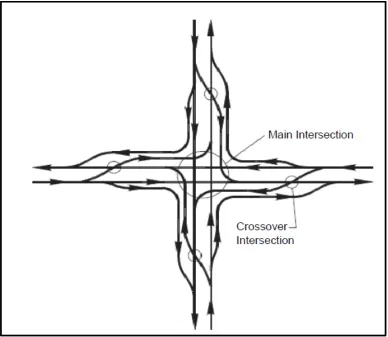
FIGURE 1.1 Continuous Flow Intersection Traffic Movements ...3
FIGURE 1.2 Vehicle Conflict Points Comparison for Conventional & CFI Intersection
Designs ...4
FIGURE 3.1 Site Location Boundaries Shown in West Valley City, UT ...21
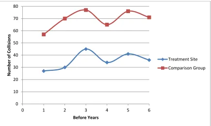
FIGURE 3.2 Collision Trends for Before Years of Comp. Group and Treatment Site(s)
...39
FIGURE 4.1 Aerial Photo of CFI in Loveland, CO ...52
FIGURE 4.2 Collision per 3 month Period for Each Site ...57
FIGURE B.1 Colorado Treatment Site, Before Period ...244
FIGURE B.2 Colorado Treatment Site, After Period ...245
FIGURE B.3 Baton Rouge, LA Treatment Site, Before Periods...246
FIGURE B.4 Baton Rouge, LA Treatment Site, After Period...247
FIGURE B.5 Lafayette, LA Treatment Site, Before Period ...248
FIGURE B.6 Lafayette, LA Treatment Site, After Period ...249
FIGURE B.7 Natchez, MS Treatment Site, Before Period ...250
FIGURE B.8 Natchez, MS Treatment Site, After Period ...250
FIGURE B.9 West Valley City, UT Treatment Site, Before Period ...251
FIGURE B.10 West Valley City, UT Treatment Site, After Period ...252
FIGURE D.2 Access Points at the Intersection of Airline Hwy. and Siegen Ln. Baton Rouge,
LA ...258
FIGURE D.3 Access Points at the Intersection of Johnson St. and Camellia Blvd. Lafayette,
LA ...259
FIGURE D.4 Access Points at the Intersection of John R. Junkin Dr. and Sgt. Prentiss Dr.
Natchez, MS ...260
1 INTRODUCTION
1.1 Problem Definition
Congestion continues to slow down the traffic flow along the arterials of America. People
spend valuable time waiting at traffic signals, frustrated at the loss of productivity and
motion waiting for their turn. Growing travel time delay and inefficient allocation of green
time remain problems despite advances in signal timing technology. Specifically, left turn
phases take too much time away from the major through movements and increase the signal
cycle length. This increases delay and travel time for all vehicles.
Conventional solutions for congestion include optimizing signal cycle length or adding
additional through and turn lanes. These solutions can offer significant improvements, but
can be unfair to all intersection users or expensive. Signal timing changes require stealing
time from one group of traffic for another. Additional lanes of traffic can be expensive,
affecting surrounding development. With growing congestion, collisions are also an epidemic
on the roadways of America. In 2008, 37,261 fatalities occurred on roadways in the United
States (1). In 2006, 23% of fatal crashes occurred at intersections (1). Conventional solutions
such as median separation and controlled right of way access can help decrease collisions but
additional solutions are needed.
This paper looks at the collision effects before and after the installation of a continuous flow
intersection (CFI) to see whether the intersection actually reduces collision frequency and/or
severity. A CFI reroutes the left turns, at one, two, or four approaches, across the opposing
through traffic at a crossover signal prior to the main signal to decrease the number of signal
phases at the main signal. Only partial CFI designs have been installed across the country
thusfar. This design requires the addition of two median crossovers per arterial with signals
to allow the left turn traffic to cross the opposing through traffic. Then, the left turns move
within the same signal phase as the through traffic at the main signal. Right turn ramps are
also included to merge right-turning traffic which would conflict with the new combined left
turn and through phase.
Installing a CFI has been shown to improve intersection operations by decreasing observed
intersection delay up to 80% and decreasing emissions (2). CFI also have a higher capacity
than a conventional intersection which allows quicker processing of high traffic volumes.
About twenty CFI designs have been installed or are currently planned within the United
States. Most studies have focused on operational benefits and the challenges of providing
effective signing and pedestrian facilities. Based on decreased conflict points, CFI designs
are assumed to have positive safety impacts, but not many studies have tested this theory. A
couple of studies have looked at safety but only within the short term for one to two sites.
This paper will perform a before and after study looking at several CFI designs across the
country to assess whether installing a CFI will have positive effects on safety.
1.2 Background of Continuous Flow Intersection Design
FIGURE 1.1 Continuous Flow Intersection Traffic Movements (3)
The traffic movement diagram represents a full CFI design treatment where all four left turn
movements cross over the opposing through movement at every approach. Different designs
apply this treatment to one, two, or four approaches. A CFI does require an additional traffic
signal for each approach with a left turn crossover; however, these signals are easy to
coordinate with the main intersection because they only control one direction of through
traffic.
Colorado, Florida, and Michigan (4). Overall, at a CFI, fewer traffic streams will be crossing,
merging or diverging into another’s path. Each approach which implements a crossover
signal reduces the number of conflict points by 1 conflict point. Figure 1.2 shows a
comparison of the number and location of conflict points of a conventional intersection, a
partial CFI, and a full CFI. Crossing conflict points are shown in black while merging and
diverging conflict points are shown in gray and white respectively. These diagrams include
vehicular conflict points only, pedestrian and bike conflict points are not shown.
FIGURE 1.2 Vehicle Conflict Points Comparison for Conventional and CFI
Intersection Designs.
TABLE 1.1 Total Conflicts Points Listed by Location
Conventional
Partial CFI
Full CFI
Main Intersection
32 22 12
Crossover Intersection
N/A 4 8
Right Turn Ramps
N/A 4 8
Total Conflict Points
32 30 28
As shown in table 1.1, each crossover intersection deletes one conflict points, the left turn
crossing over the opposing left turn point, from the main intersection. Each right turn ramp
pulls away an additional two conflict points, the right turn diverging and merging conflict
points. This additional safety benefit suggests that the continuous flow intersection design
may be a safety treatment in addition to its known use as a congestion management solution.
Potential negative safety effects are possible because of the different operation of the CFI. At
the crossover approach, the right-turning traffic becomes permitted for all phases other than
the left turn phase for the non-crossover approach since the left-turning movements now run
in the same phase as the through traffic from the crossover approaches. Because drivers are
used to moving with the through traffic, this change could cause conflicts. Right turn ramps
are provided to allow the non-crossover approach right-turning movement to navigate around
the crossover left turns, but the end of the ramp still allows for a merging movement within
the through green time at the crossover signal. This merge point is more dangerous for
drivers since it in uncontrolled by a signal with most designs. Also, the additional signals
may mean more rear-end collisions. With these unknowns, additional study is needed to
determine the safety effects of continuous flow intersections.
constructed was also a three-legged design in Accokeek, MD which was completed in 2001
(6).
The first four-legged intersection to incorporate the CFI design is located in Baton Rouge,
Louisiana (6). This design is a partial CFI with crossover signals on two approaches. It has
been operating since March 2006 with promising results. In 2007, partial CFI designs were
completed in both Salt Lake City, Utah and Fenton, MO to help with congestion (6). With
the success of their first CFI at 3500 South and Bangerter Highway in Salt Lake City, Utah
Department of Transportation has implemented the CFI concept at several surrounding
intersections along Bangerter Highway and throughout the state. CFI designs have also been
completed in Ohio, Colorado, and Mississippi.
1.3 Research Objectives
This study looks to explore the safety implications of installing a continuous flow
intersection to fill this void in knowledge of the continuous flow design. The objectives of
this study are:
1.
To determine the safety impacts of installing a continuous flow intersection with
naïve and comparison-group analyses, and
2.
To determine whether installation of a continuous flow intersection has similar safety
results across the country.
Continuous flow intersections have proven benefits in decreasing congestion and improving
arterial travel times, but have not been subjected to rigorous safety analysis. This study hopes
to show the safety effects from the installation of continuous flow intersections. If continuous
flow intersections show safety benefits as well as congestion benefits, hopefully more of
them will be constructed across the United States. If there are no safety benefits, other
1.4 Scope
This study is limited to arterial intersections within the states which are included in this
study. Because continuous flow intersections have not been implemented uniformly across
the United States, no attempt could be made to select sites in a significant manner to
represent the different weather, development, and terrain conditions of the United States. If
continuous flow intersection installation becomes more widespread, the safety impacts
should be studied further to apply to the entire United States. Sites included in this study
have the following similar characteristics present at the intersection:
1.
Meeting of major and minor arterials with 2-3 through lanes per approach.
2.
Dedicated left and right turn lanes at multiple approaches.
3.
Suburban location on the outskirts of major urban center.
4.
High level of commercial development surrounding intersection.
The results of this study should not be applied to intersections which do not fit within this
subcategory of continuous flow intersections. An acknowledgment of the unique factors of
each individual site will be included with the analysis to attempt to analyze the significance
of other design factors such as connected service roads, right turn ramps, and surrounding
access to parcels.
1.5 Organization of Thesis
This thesis will include five chapters. Chapter one presented an introduction to the
2 LITERATURE REVIEW
This paper presents existing literature on two topics: the continuous flow intersection and
safety study methodology.
2.1 Continuous Flow Intersection
Research on the CFI has been completed for both operational and safety impacts of the
design. VISSIM and other modeling programs have been used to compare the operation of
the CFI to conventional intersections as well as other unconventional options. Safety studies
have been completed using both surrogate analysis and collision data for a limited number of
sites. Only the more recent studies have been included in this literature review.
2.1.1 Operational Impacts
Multiple studies have looked at the CFI’s performance compared with other intersection
types for various volumes. In most cases, the CFI has performed better with reduced delay
and increased vehicle throughput. Other parts of the design such as pedestrian facilities and
signing have also been studied to determine the most effective usage within a CFI.
Esaway and Sayed (3) used VISSIM to compare the reduction in delay of both the CFI and
the upstream signal crossover (USC) to a conventional intersection. Specific lane
configuration was not shown, but generally an exclusive turn lane and two through lanes
were included on each approach. In all cases, the greatest delay reduction was seen in the CFI
model with the USC model also showing reduced delay in comparison to the conventional
intersection model. The authors attribute this difference to the greater storage length space
available for left turns in the CFI design.
provided higher throughput values in all but one case. The CFI also was shown to have fewer
stops for both through and left turn movements in all cases. This study concludes that the CFI
in general outperforms the PFI, but the PFI could be preferable in certain situations where
right of way is limited in certain quadrants.
Olarte et. al. (8) compares the operational performance of the diverging flow intersection, the
continuous flow intersection, and a new left turn bypass intersection. The left turn bypass
intersection removes the right turn ramps at a continuous flow intersection, having right turns
make their turn at the main intersection, and creates a left turn bypass lane where left turns
only go through two crossover intersections downstream of the main intersection. The results
show that the continuous flow intersection operates with less delay in almost all cases. The
other two options performed with better delay in some low to medium volume cases.
Because these designs are meant for high traffic volumes, the continuous flow intersection is
recommended as the best solution in most cases.
Jagannathan and Bared (9) completed a study looking at the performance of pedestrian
facilities for continuous flow intersections. This study addressed the complication caused by
the inclusion of right turn ramps which causes pedestrians to have to make three separate
crossings for a one directional crossing. Their VISSIM analysis showed that the performance
of the system is tied to whether the right turn ramps are signalized and how easy it is for
pedestrians to get to the median refuge for the main street crossing movement. In their
analysis, they found that an acceptable pedestrian level of service could be provided with
their modeled geometries.
ground-mounted signing, and did not show a statistically significant benefit in using overhead signs.
Also, no problems were found with the minor street through movement blocking the main
street left turns. Overall, this research needs to be confirmed with a larger number of
participants.
2.1.2 Safety Impacts
Safety studies have looked at a limited number of sites to try to determine if there are any
significant safety benefits gained from installing a CFI. Because limited data were available
at the time, more thorough research is needed to include additional sites with further years of
data.
Park and Rakha (12) looked at both the environmental impacts of installation of a CFI and
early safety impacts from driver confusion based on the differences between a CFI and a
conventional intersection. Using VISSIM and INTEGRATION software, both CFI and
conventional intersection models were loaded with a variety of flows to assess environmental
impacts. Decreased emissions were shown in all CFI cases, with greater effects seen as traffic
volumes increased. A conflict study was also completed using video analysis from two sites,
partial CFIs in Baton Rouge, LA and West Valley City, UT. This analysis showed a 50%
reduction in conflicts at the sites from the initial opening of the intersections to one year after
the opening of the intersections. Because this study looks only at after data, conclusions
could not be draw about the CFI’s safety impacts from before to after period.
positive feedback on the reduction of travel times, increased safety, and similar or better
access to surrounding parcels.
2.2 Safety Study Methodology and Correlations
To inform the safety study, background research was reviewed on safety study methodology
and the correlation of conflict and conflict points to decreased collision rates. This will show
the applicability of an observational before and after study to the safety effects of installing a
CFI.
2.2.1 Safety Study Methodology
Hauer (14) will be used as the main methodology for the overall method to treat collision
data as well as the naïve and comparison group before and after study. In sorting collision
data, Hauer (14) emphasizes the importance of correctly defining target collisions to show
the overall safety treatment. By reducing the number of included types of collisions too
much, the number of overall crashes can become so small that it becomes hard to analyze.
Accounting for differences in reported data is also important because differences in crash
reporting can cause different data sources to appear to be safer when collision reductions are
really due to a different reporting threshold. Hauer includes a method to avoid these missteps
when compiling data.
The naïve before-and-after study compares the collision data from the before and the after
period while assuming that nothing other than the treatment has changed (14). This
baseline to estimate the fluctuations in collision rates without the installation of the treatment.
These methods will be further explained within the Methodology section.
Ott et al’s safety study looking at both signalized and unsignalized superstreets includes this
methodology (20). This study uses Hauer’s four-step method adjusting with traffic factors
and using the comparison group method. This study also includes the empirical Bayes
method to correct for possible regression to the mean. Commuter surveys are also included in
the analysis. The results suggest that especially unsignalized superstreets do have safety
benefits for all types of collisions.
The traffic conflict method is now accepted as a substitute for an observational before and
after study, using collision surrogates to estimate the safety of an intersection or feature. This
section will look at the applicability of this method to the current study of the safety of
continuous flow intersections.
Hauer and Garder (15) discuss the validity of the traffic conflicts technique in estimating the
safety of an entity. First, safety has been defined to be the expected number of collisions by
severity on an entity per unit of time (15). To use conflicts to estimate safety, the number of
conflicts must be related back to the expected number of collisions. According to Hauer and
Garder, the effectiveness of the conflicts technique depends on how constant the accident to
conflict ratios are from similar entity to entity, which relies on the variance of this ratio (15).
Glautz and Migletz have determined different collision to conflict ratios for several different
conflict types (16).
Many studies look at a certain segment of overall crashes at an intersection, such as only
injury and fatal crashes to attempt to determine whether the severity of crashes is decreasing
at an intersection as well as a decreasing frequency. According to the following sources,
determining whether a reduction in crash severity or a reduction in crash frequency has taken
place when comparing crash frequencies is difficult because of variable reportability.
According to Hauer (17), reportable crashes normally include only crashes with significant
property damage and collisions involving injury or death. Among this subset, significant
numbers of crashes go unreported. Hauer and Hakkert estimate that 20% of severe injury,
50% of minor injury, and 60% of no-injury crashes are not reported (18). Savolainen et al
(19) makes the point that the reported crash sample is not random because the reportability
changes based on the outcome of each crash which means that the proportion of injury within
all crashes is most likely not the same as that within reported crashes. This makes it difficult
to determine what the proportion of injury crashes is within a given sample over time. Hauer
maintains that the cause of an increase or decrease in crashes between crash frequency and
crash severity can only be determined if the probability of the types of crashes being reported
is known and taken into account (17). With this information, this study will not separate
crashes by severity but will make judgments based on the changing collision frequency as a
whole. Reportability will be discussed later in the Methodology section as it relates to
location differentiation.
3 METHODOLOGY
This chapter will discuss the data collection and safety analysis methods used to determine
the safety impacts of installing continuous flow intersections. A complete crash data set will
be included in Appendix A. This section will also address the potential variation of results
among sites across multiple states and how this effect will be studied through the use of
multiple analysis groupings. First, this section will include information on how appropriate
treatment sites were selected from the various continuous flow intersections across the
country. Data collection techniques and the data limitations will also be included in the
chapter. Comparison site selection criteria will also be discussed. Further step by step details
will be included for both the naïve and comparison-group observational before-and-after
study methods.
3.1 Site Selection
Because continuous flow intersections have not been accepted as a standard intersection
treatment and have not been applied in many locations, the number of potential treatment
sites to study is limited. Although continuous flow intersections have been widely used in
Mexico, where they were invented, this study is limited to sites within the United States. This
criterion relies on the assumption that design standards and driver behavior will be similar
within the United States. Within the United States, 10 or so continuous flow intersections
have been installed at the time of this study. This study will use two main criteria to select
which continuous flow intersections to study. First, any site with unusual continuous flow
elements, such as jughandles, will be eliminated as outside the normal continuous flow
design standard. All sites must also have been completed and have available at least one year
and three months of collision data after the end of construction of the continuous flow
With these criteria in mind, 7 sites were initially selected to be analyzed for this study. Other
sites such as those in New York and Maryland were eliminated because they were
three-legged designs with unique right of way concerns which made them dissimilar to partial or
full continuous flow designs. Sites in New Jersey will not be used because the design
includes a jughandle which, as an additional unconventional design element, would make it
more difficult to discern what amount of change in the collisions was due to the installation
of the continuous flow intersection. Several continuous flow intersections are also being
installed in Taylorsville and Orem, Utah as well as along Bangerter Highway in West Valley
City UT, forming what could be considered a continuous flow corridor; however, only one of
the sites was installed with enough after data to be included in this study. A full CFI design
has been installed in Taylorsville, UT, but did not have the necessary after data. Further
research should be conducted to determine the safety effects of the use of continuous flow
intersections as a corridor and with full continuous flow designs in the future.
From studying aerial maps of the seven initial sites, the author eliminated two additional sites
which were not typical continuous flow intersections. The Fenton, MO site included the
extension of Gravois Bluffs Rd. to the intersection of Summit Rd. and MO-30. This meant
adding a leg to the existing 3-legged intersection, adding a new traffic source with the
development along Gravois Bluffs Road. Also, in Springboro, OH, the CFI construction was
completed concurrently with the construction of a new diamond interchange directly
TABLE 3.1 Study Sites by Location and Number of Crossovers
Street 1
Street 2
Location
Number of
Crossovers
US 34/Eisenhower
Blvd.
Madison Ave.
Loveland, CO
2
US 61/Airline Hwy.
LA 3246/Siegen Ln.
Baton Rouge, LA
2
US 167/Johnson St.
Guilbeau Rd./Camellia Blvd. Lafayette, LA
2
US 61/US 84/US
425/John R Junkin Dr.
US 61/US 84/ Sgt. Prentiss
Dr. Natchez,
MS
1
UT 154/ Bangerter
Hwy.
UT 171/ W. 3500 S.
West Valley City,
UT 2
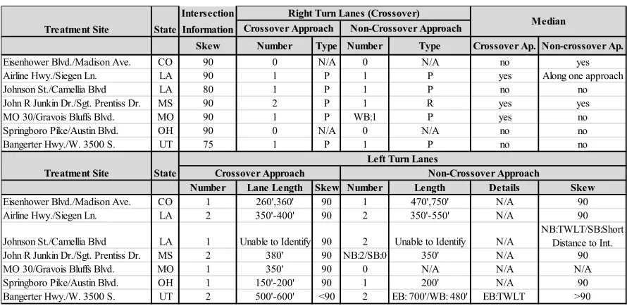
In Table 3.2 and 3.3 below, site information regarding turn lanes, lane lengths and median
type is provided for the intersection prior to CFI construction and after construction
respectively.
TABLE 3.2 Existing Intersection Design Criteria Table
Where:
P = Permitted turning movement at main intersection.
TWLT = Two way left turn lane.
Skew Number Type Number Type Crossover Ap. Non-crossover Ap.
Eisenhower Blvd./Madison Ave. CO 90 0 N/A 0 N/A no yes Airline Hwy./Siegen Ln. LA 90 1 P 1 P yes Along one approach
Johnson St./Camellia Blvd LA 80 1 P 1 P no no
John R Junkin Dr./Sgt. Prentiss Dr. MS 90 2 P 1 R yes yes
MO 30/Gravois Bluffs Blvd. MO 90 1 P WB:1 P yes no
Springboro Pike/Austin Blvd. OH 90 0 N/A 0 N/A no no
Bangerter Hwy./W. 3500 S. UT 75 1 P 1 P no no
Number Lane Length Skew Number Length Details Skew
Eisenhower Blvd./Madison Ave. CO 1 260',360' 90 1 470',750' N/A 90 Airline Hwy./Siegen Ln. LA 2 350'-400' 90 2 350'-550' N/A 90 Johnson St./Camellia Blvd LA 1 Unable to Identify 90 2 Unable to Identify N/A
NB:TWLT/SB:Short Distance to Int. John R Junkin Dr./Sgt. Prentiss Dr. MS 2 380' 90 NB:2/SB:0 350' N/A 90
MO 30/Gravois Bluffs Blvd. MO 1 350' 90 0 N/A N/A N/A
Springboro Pike/Austin Blvd. OH 1 150'-200' 90 1 200' N/A 90 Bangerter Hwy./W. 3500 S. UT 2 500'-600' <90 2 EB: 700'/WB: 480' EB:TWLT >90
Treatment Site State
Left Turn Lanes Right Turn Lanes (Crossover) Intersection
Information State
Treatment Site
R = Ramp turning movement separated from traffic flow at signal.
NB, SB, EB, WB = Northbound, Southbound, Eastbound, and Westbound
approaches.
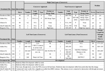
TABLE 3.3 CFI Design Criteria Table
Where:
RIRO = Right in right out access.
After selecting treatment sites, comparison sites also needed to be selected. Comparison sites
model the change over time of other factors which affect collision frequency such as
seasonality and historic trends. To find good comparison sites which better match the
treatment sites and their base conditions, the following four criteria were used:
Skew Number Lane
Length Type
Feature at
Merge Point Number Lane Length Type
Feature at
Merge Point X-over Non-X-over
Eisenhower Blvd. CO 90 1,0 N/A P None 1 400'-450' R Merge Tapers yes yes Airline Hwy. LA 90 1 550',N/A P SB: Merge Taper 1 550' R,R with
meter
Merge Taper,
Signal Control yes yes Johnson St. LA 80 0,2 N/A P None 1 N/A, 550' P None yes no John R Junkin Dr. MS 90 2 N/A P None 1 N/A, 550' P,R None yes yes Bangerter Hwy. UT 75 1 N/A P Right lanes 1 500',600' R Right lane tapers yes no
Treatment Site State
Number Length Skew Number Length Skew
Eisenhower Blvd. CO 1,2 250'-275' 90 1 380',670' 90 175'-225' Airline Hwy. LA 2 400'-430' 90 2 300',450' 90 300'-350'
Johnson St. LA 2 360',460' EB:>90,WB:<90 2 NB: 370',
SB:160' 90 300',400' John R Junkin Dr. MS 2 250' 90 2 450',300' 90 220'
Bangerter Hwy. UT 2 280' <90 2 700'/WB: EB: >90 200'
Treatment Site State
Eisenhower Blvd. CO Airline Hwy. LA Johnson St. LA John R Junkin Dr. MS Bangerter Hwy. UT
Left Turn Lanes (Crossover) Treatment Site
Median
Development
Relatively Minor Development visible by aerial. Relatively Minor Development visible by aerial.
Friar Lane, through street, is now the WB crossover left turn lanes. Relatively minor development visible from aerial other than this change. Commercial Center south of int. originally accessible from RIRO entrance. This entrance is now connected to intersection with through movement. Relatively Minor Development visible by aerial.
Details
N/A 1 SB LT connects
to service road. EB LT connects to
new. int.
Sharp Left Turn
Details
N/A N/A
NB:TWLT/SB:Short Distance to Int.
N/A EB:TWLT Storage Length for Through Traffic Prior to Crossover Left Turn Lanes (Non-Crossover)
Right Turn Lanes (Crossover)
Crossover Approach Non-Crossover Approach
1.
Four-legged, signalized, conventional intersections,
2.
Close in location to the treatment site,
3.
Along the same or a very similar arterial, and
4.
Similar collision trend, as tested by the odds ratio.
For all the treatment sites, several comparison sites were selected which fit the first three
criteria. By choosing comparison sites with similar intersection configurations, the author
expects to see the same types of collisions. Proximity of location makes it likely that the
treatment and comparison sites experience similar weather conditions, traffic volume
changes, and historic trends. Also, since CFIs are most effective at the intersection of two
major arterials, the author chose sites along the same or similar arterials as what could be
considered alternative options for a CFI installation. Explanation of the odds ratio procedure
is located in Section 4.2.
3.2 Data Collection and Analysis
This section discusses the data collected for use in this study and any corrections or changes
that were made to the raw data for use in this specific study. For each site, the author
requested as-built drawings, collision reports, and average annual daily traffic volumes
(AADT)s along both arterials from the state departments of transportation. The as-built
drawings provided information about each site’s unique design. Collision data from before
and after the construction of the treatment sites was necessary from both treatment and
comparison sites to complete the safety analyses described above. The naïve method with
traffic factors required AADT information along both arterials spanning the construction
period for the treatment sites.
3.2.1 Geometric Data
3.2.2 Collision Reports
The author received collision data containing necessary parameters per crash for each of the
five sites. The formats differed slightly, but generally the same information was included for
each site. These crash parameters included date and time of crash, crash type, first harmful
event, crash severity, weather, distance from intersection, street names, direction of vehicles,
number of vehicles, crash descriptions, crash number, etc. The crash data from Loveland,
CO, Baton Rouge, LA, and Lafayette, LA did not include specific crash severity information
but did include three categories: fatal, injury, or property damage only. After receiving this
data for all the sites, the crash compilations were revised based on duplication of reports, site
location boundaries, consolidation of crash parameters, and before and after time periods of
study.
3.2.2.1 Duplicate Reports
Multiple sites included different crash queries with duplicate reports based on the state’s
reporting system. Some states had to run multiple queries to get crashes along both sides of a
median with a distance query and also if there were multiple different city/state street names.
Duplicate reports were eliminated by matching crash identification numbers as well as date
and time of crash.
In West Valley City, UT, the crash data included crash reports occurring within minutes of
each other. The author determined the relationship between the crashes based on the crash
description and eliminated the secondary crash where necessary. Utah’s system also included
separate police follow-up reports based on hit and run crashes or other criminal activities.
The author eliminated these reports when identified by duplicate crash identification
numbers, time of crash, and crash description.
of Transportation. While some duplicates were included, they were eliminated by checking
crash time as well as crash severity and type where necessary.
3.2.2.2 Site Location Boundaries
FIGURE 3.1 Site Location Boundaries Shown in West Valley City, UT
The author used those boundaries for both the before and after periods. The author requested
collisions occurring within the site description noted above and confirmed that the collision
sample fit this site description for four of five sites. Distance information was not provided as
a crash parameter from Colorado, but the author worked with a representative from the City
of Loveland Traffic Department who added collisions by hand based on the site description.
The collision sample for both sites in Louisiana included much more data than the required
sample. The collisions outside the site boundaries were therefore deleted from the sample.
Mississippi and Utah provided samples which fit this description upon verification.
A
B
3.2.2.3 Consolidation of Crash Parameters
Because this study includes sites from multiple states, the format and justifications for a
crash report were different for each site. For the overall site analysis, the format needed to be
merged to include categories such as crash severity and collision classification. Also, when
possible, the author wanted to insure that the sample of collisions from each state was based
on similar regulations for crash reporting.
Each state had different coding standards for crash severity and collision type. Some of the
sites, including those in Louisiana, listed collision type by several codes including direction
of travel for each vehicle, action prior to collision, and location of damage. The author
translated these codes into several collision categories such as rear end slow or stop, rear end
turn, angle collision, left turn same roadway, left turn different roadway, right turn same
roadway, right turn different roadway, sideswipe same direction, sideswipe opposite
direction, parking, backing up, other, etc. Because of difficulty distinguishing between the
left turn, right turn, and angle categories for some sites based of the data parameters
provided, the author combined these categories for the overall site analysis. Additional
details of this consolidation are included within Appendix A with the complete collision data
set.
reporting threshold but reports property damage per vehicle as none, light, or heavy (23).
Utah includes a reportable crash yes or no box to indicate whether a crash has passed its
$1000 property damage threshold, but it specifically discusses the fact that some agencies
complete reports on all reported crashes regardless of this reporting threshold (24). The
author could not correct for this difference in the reporting standards by state for the overall
site analysis and recognizes this as a bias in the overall collision sample. Any changes per
state in the reporting threshold should be accounted for by the comparison group method
since it also would reflect that change.
3.2.2.4 Before and After Time Periods
Hauer suggests using three to five years of before and after data for observation before and
after studies (14). With this recommendation, the author requested and included up to 6 years
of before and after data for each treatment site. Many of the sites had less than six years of
before and after data available due to archived data or construction completed near the
treatment sites.
Colorado completed archiving its collision data prior to June 2006, providing four years of
before data. In West Valley City, UT, the CFI opened to the public in September 2007, but a
new widening project along 3500 S began in mid-March 2009, allowing only one year of
after data to be included to avoid safety effects from the other factors associated with this
new construction. In Baton Rouge, LA, the construction period for the CFI overlapped with
Hurricane Katrina. This disaster halted construction for several months, pushing back the
completion date to March 2006. Because the construction was completed more than 6 months
after Hurricane Katrina, no additional time was subtracted from the after time period to
replicate the different traffic patterns associated with an evacuation. Because the hurricane
took place once construction had already started, the before period data was also unaffected.
avoid the initial effects of the treatment when drivers are still unfamiliar with the new
intersection configuration. Generally, a year should be allowed for the warming up period,
but some of the most recently constructed sites in Lafayette, LA, and Loveland, CO, only had
enough crash data available to include a three-month warming up period and one year of
after data. Table 3.4 shows the number of years of before and after data included for all
individual site analyses along with the exact dates of these time periods.
TABLE 3.4 Before and After Time Periods for Treatment Sites
Site Location
Before
Years
Before Period Dates
After
Years
After Period Dates
Loveland, CO
4
06/01/2006 - 05/31/2010
1 03/01/2011
-
02/29/2012
Baton Rouge,
LA
5 02/01/2000
-
01/31/2005
5 06/01/2006
-
05/31/2011
Lafayette, LA
4
01/01/2006 - 12/31/2009
1 05/15/2011
-
05/14/2012
Natchez, MS
4
01/01/2005 - 12/31/2008
2 03/04/2010
-
03/03/2012
West Valley
City, UT
6
02/01/2001 - 01/31/2007
1 12/16/2007
-
12/15/2008
This analysis assumes that the treatment effect remains relatively constant after the
construction of the CFI, averaging the effects over the after period for the analysis.
Additional data increases the sample size of collisions, but can show incorrect trends if the
other factors associated with changes in collisions do not remain the same or are correctly
included in the analysis.
The author completed both individual and overall site analyses for all methods where
possible. The individual site results show variation based on the specific design of each site,
which is especially important since these sites are located in different states and therefore
were designed differently. Additional details of the different designs will be discussed in the
results section. The overall site results allow for a larger sample of collisions where
changes in these categories which would not be possible for these categories with individual
sites. The author used a limited three years of before data and up to three years of after data
for the overall site analysis to balance the need for a larger sample of collisions and the need
for sites to contribute evenly to the overall site analysis. Three of five sites had only one year
of after data. The sites in Natchez, MS and Baton Rouge, LA had additional years of data
which showed a decreasing trend in collisions. Up to three years of after data from these two
sites was included to show the effects of the continuous flow intersection over time. This
allowed all five sites to contribute significantly to the overall site analysis. Five years of after
data were available for the Baton Rouge CFI, but the last two years were not included
because that volume of collisions would overwhelm the overall site analysis and overshadow
the after collisions contributed by other sites. A safety study completed on unsignalized
superstreets applied a similar method including varied years of before and after data in
overall site analyses (20).
3.2.3 Traffic Volume Data
State traffic volume maps were used to get AADTs for both the minor and major arterials at
each treatment site. AADTs were available every 2-3 years for each site. The author used
linear regression models to interpolate years where specific AADTs were not provided.
3.3 Explanation of Safety Analysis Types
This section will explain the methodology used for several types of safety analyses included
in this study: naïve method, naïve method with traffic factors, comparison group method, and
severity index method.
included to correct for regression to the mean since CFI designs chosen for the included sites
were based on congestion problems, not safety issues. Therefore, regression to the mean bias
should not affect these sites.
3.3.1 Naïve Method
The naïve method acts as a baseline index of effectiveness for the continuous flow
intersection treatment, without correction factors. This method attributes all changes in
collision frequency to the treatment, although other factors affect collision frequency
including historical trends, regression to the mean in some cases, seasonality, weather, and
traffic patterns. By avoiding inclusion of other factors, this method offers an artificially low
variance around the estimate of the collision change (14). The effects of these other factors
are then assumed to be due to the safety treatment which is false. Hauer’s four-step method is
replicated for this study to predict what the safety of an entity in the after period would have
been without the treatment to measure safety impacts (14). The four steps of this method are
listed below.
1.
Estimate
λ
, expected target collisions in the after period at treated entity, (14, eq.
7.1) and predict
π
, expected target collisions in the after period without treatment,
(14, eq. 7.1) using , a ratio of the duration of the after period to the duration of
the before period.
2.
Estimate Var (
λ
), (14, eq. 7.2) and Var (
π
), (14, eq. 7.2).
3.
Estimate
δ
, reduction in the expected number of target accidents in the after
period assumed due to the treatment, (14, eq. 6.1) and
θ
, the index of effectiveness
or the ratio of what safety was with the treatment to what it would have been
without the treatment, (14, eq. 6.3).
4.
Estimate Var(
δ
), (14, eq. 6.2) and Var (
θ
), (14, eq. 6.4).
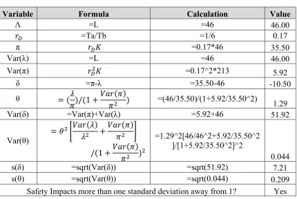
TABLE 3.5 Naïve Method Example Calculation – Utah Site
Variable
Formula
Calculation
Value
Λ
=L
=46
46.00
=Ta/Tb =1/6
0.17
π
=0.17*46
35.50
Var(
λ
) =L
=46 46.00
Var(
π
)
=0.17^2*213
5.92
δ
=
π
-
λ
=35.50-46
-10.50
θ
/ 1
=(46/35.50)/(1+5.92/35.50^2)
1.29
Var(
δ
) =Var(
π
)+Var(
λ
) =5.92+46
51.92
Var(
θ
)
/ 1
=1.29^2[46/46^2+5.92/35.50^2
]/[1+5.92/35.50^2]^2
0.044
s(
δ
) =sqrt(Var(
δ
)) =sqrt(51.92)
7.21
s(
θ
) =sqrt(Var(
θ
)) =sqrt(0.044)
0.209
Safety Impacts more than one standard deviation away from 1?
Yes
Where:
L = Number of collisions occurring at treatment site in the after period,
Ta = duration of after period, years,
Tb = duration of before period, years, and
K = Number of collisions occurring at treatment site in the before period.
Using this method, an estimate of both the reduction in collisions and the index of
effectiveness due to the treatment can be calculated. This method estimates the number of
collisions without the treatment per year to be the yearly average of the before period
crashes, since this method assumes nothing else would affect the collision frequency.
3.3.2 Naïve Method with Traffic Factors
information will be used to calculate a safety performance function relating traffic volume
changes to collision effects. Removing the traffic bias from the raw data allows the results to
show any collision frequency effects due to factors other than changing traffic volumes (14).
3.3.2.1 Choosing a Safety Performance Function
The function relating traffic changes can take several forms (14). In this case, the safety
performance functions from the Highway Safety Manual (HSM) were used as they have been
calculated based on aggregate data from similar intersections. The Suburban and Urban
Arterial Intersection safety performance functions were used here since they represent the
most similar intersection types to the treatment sites chosen for this study. Eq. 3.2 shows the
calculation for the safety performance function requiring a weighted average of AADTs
along both arterials in the before and after period. Since the before and after periods start in
various months, any year within the before and after time periods of at least two months was
used to calculate the weighted average of AADTs.
Eq. 3.2:
∗ ∗(27)
Where:
= Safety Performance Function from the HSM (27),
a,b,c = regression constants listed for suburban and urban arterial intersections (27),
=Weighted average of AADT along major arterial of treatment site, and
=Weighted average of AADT along minor arterial of treatment site.
A safety performance function value is calculated for both the before and after periods using
the AADT information from these time periods. More information on the traffic volume
information included and specific safety performance function calculations for all
TABLE 3.6 Safety Performance Function Example – Utah Site
Street Name
Before After
Bangerter Hwy, major
49939 49170
W. 3500 S. , minor
33589 34265
a -10.99
b 1.07
c 0.23
19.75 19.51
The weighted average AADTs along both arterials in Utah decreased from the before to after
period, resulting in a decrease in the safety performance function (SPF). The necessary traffic
factor is calculated as shown below in Eq. 3.3.
Eq. 3.3:
__
(14, eq. 8.5)
Where:
= safety performance function evaluated at the weighted average of traffic
volumes in the after period and
= safety performance function evaluated at the weighted average of traffic
volumes in the before period.
The HSM also recommends that a calibration study be completed to model outside factors,
but in this case, with sites across multiple states with different weather patterns, design
factors, and terrain, finding the commonalities to complete a calibration would be difficult.
This should not affect the results of this study since the safety performance functions are
used to create a ratio and the same relative difference would be applied in the before and
after period.
3.3.2.2 Naïve Method with Traffic Factors Steps
1.
Collect AADTs from both arterials during before and after periods.
2.
Calculate
for before and after periods using weighted average
AADTs.
3.
Calculate
, adjustment factor for traffic volume data (14, eq. 8.5).
4.
Estimate
λ
, expected target collisions in the after period at treated entity,
(14, eq. 7.1) and predict
π
, expected target collisions in the after period
without treatment, (14, Table 8.2) using only , a ratio of the target
collisions in the after period to the target collisions in the before period,
eq. 3.1 and
, an adjustment factor based on changing traffic volumes,
eq. 3.3
5.
Estimate Var(
, (14, eq. 8.6), Var (
λ
), (14, eq. 7.2), and Var (
π
) (14, eq.
Table 8.2).
6.
Estimate
δ
, reduction in the expected number of target accidents in the
after period assumed due to the treatment, (14, eq. 6.1) and
θ
, the index of
effectiveness or the ratio of what safety was with the treatment to what it
would have been without the treatment, (14, eq. 6.3).
7.
Estimate Var(
δ
), (14, eq. 6.2), and Var (
θ
), (14, eq. 6.4).
Because of the functional form of the safety performance function chosen, calculating
Var(
requires Eq. 3.4 relating the traffic factor variance to the variance of the weighted
averages of the AADT information used.
Eq. 3.4:
(14, eq. 8.6)
Where:
Var r
= Variance of traffic factor
r
,
r
= Traffic Factor based on traffic volume changes from before to after period,
= Derivative of f(B) evaluated at weighted average of AADTs in the before period,
= Variance of weighted average AADT in the after period, and
= Variance of weighted average AADT in the before period.
Because the safety performance function uses AADTs along both arterials, partial derivatives
of function f(AADT) are evaluated at the weighted average AADT for the minor and major
arterials; further details of this process are included in Appendix C. Tables 3.7 and 3.8 show
an example calculation for the West Valley City, UT site.
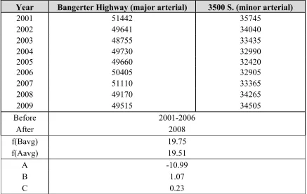
TABLE 3.7 Raw Traffic Data – Utah Site
Year
Bangerter Highway (major arterial)
3500 S. (minor arterial)
2001 51442
35745
2002 49641
34040
2003 48755
33435
2004 49730
32990
2005 49660
32420
2006 50405
32905
2007 51110
33365
2008 49170
34265
2009 49515
34505
Before 2001-2006
After 2008
f(Bavg) 19.75
f(Aavg) 19.51
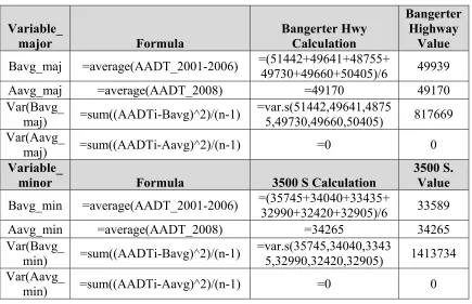
TABLE 3.8 Weighted Average and Variance Calculations – Utah Site
Variable_
major
Formula
Bangerter Hwy
Calculation
Bangerter
Highway
Value
Bavg_maj =average(AADT_2001-2006)
=(51442+49641+48755+
49730+49660+50405)/6
49939
Aavg_maj =average(AADT_2008)
=49170
49170
Var(Bavg_
maj)
=sum((AADTi-Bavg)^2)/(n-1)
=var.s(51442,49641,4875
5,49730,49660,50405)
817669
Var(Aavg_
maj)
=sum((AADTi-Aavg)^2)/(n-1) =0
0
Variable_
minor
Formula
3500 S Calculation
3500 S.
Value
Bavg_min =average(AADT_2001-2006)
=(35745+34040+33435+
32990+32420+32905)/6
33589
Aavg_min =average(AADT_2008)
=34265
34265
Var(Bavg_
min)
=sum((AADTi-Bavg)^2)/(n-1)
=var.s(35745,34040,3343
5,32990,32420,32905)
1413734
Var(Aavg_
min)
=sum((AADTi-Aavg)^2)/(n-1) =0
0
Where:
Bavg_maj = Weighted average of AADTs during before period at major arterial leg,
Aavg_maj = Weighted average of AADTs during after period at major arterial leg,
Bavg_min = Weighted average of AADTs during before period at minor arterial leg,
and
Aavg_min = Weighted average of AADTs during after period at minor arterial leg.
TABLE 3.9 Naïve Method with Traffic Factors Example – Utah Site
Variable
Formula
Calculation
Value
= after duration/before duration
=1/6
0.17
=f(Aavg)/f(Bavg) =19.51/19.75
0.99
Cb_maj
,
19.75
.0.00042
Cb_min
,
19.75
.0.00014
Ca_maj
,
19.51
.0.00043
Ca_min
,
19.51
.0.00013
Λ
=L
=46
46
Π
=0.17*0.99*46 35.08
Var(
λ
) =L
=46
46
Var(f(Bavg))
__
0.00014 ∗
1413734
0.00042 ∗ 817669
0.17
Var(f(Aavg))
__
0.00013 ∗ 0
0.00043 ∗ 0
0
Var(rtf)
0.99
.. .