Vol 6, No 11 (2015)

Available online throug

ISSN 2229 – 5046

A STOCHASTIC MODEL FOR ANTIGENIC DIVERSITY THRESHOLD

WITH TWO SOURCES OF HIV INFECTION

S. C. PREMILA

1

_{, S. SRINIVASA RAGHAVAN*}

2

1

_{Mar Gregorios College of Arts and Science, Chennai – 600 037, India.}

2

_{Veltech Dr. R.R. & Dr. S.R. Technical University, Avadi, Chennai, India.}

(Received On: 06-04-15; Revised & Accepted On: 13-05-15)

INTRODUCTION

In the study of HIV infection one of the aspects of study is to obtain the estimate of the time to seroconversion. since the time of HIV conversion is random, one would expect that the seroconversion distribution would have an important impact on the course of the HIV epidemic. The transmission of HIV occurs through different modes but the most commonly and widely prevalent mode of transmission is the home or heterosexual contacts. The concept like incubation period, Latency period has been discussed by author like Anderson (1988) and others. Most of the result has been on the basis of the assumption that the sexual contact alone is the only source of transmission of HIV. Ahlgren et al. (1987) have introduced a compartmental model of HIV transmission via sexual contact, needle sharing and infected blood products.

In this paper the cumulative effect of HIV transmission through sexual contacts as well as needle sharing upon the break down of the immune system is study through shock models. Hence it is possible that on a every occasion of sexual contacts and using unsterile needle, there is a possibility of HIV transmission and it is likely that more and more of HIV are getting transmitted from the infected person to the uninfected. The antigenic variation would be on the increase. If the antigenic diversity crosses a particular level, which is, known as antigenic diversity threshold, then there is a collapsed of the immune system and seroconversion immediately take place. The antigenic diversity threshold models has been discussed by Nowak and May (1990) and Stilinakis et. al (1994).

The concept of cumulative damage process is used to determine the mean and variance of period remaining in the seronegative state after an individual has a certain number of contacts with an infected partner a detail account of same would be seen Esary et.al (1973). A stochastic model based on the cumulative damage process is derived and using this model it is possible to obtain the expected time to seroconversion and its variance according to Premila and Srinivasan Ragavan (2014), proposed a stochastic model for the seroconversion time of HIV transmission in which the antigenic diversity threshold follows exponential distribution, it is prove the examine the impact of the exposures to two-sources of infections on the expected time to seroconversion and its variance. Numerical illustration for different combination of the parameter involve in the distribution of the random variables used in the model.

Assumption of the Model

(i) An uninfected partner has a sexual contacts with on infected person and also shares unsterile needles for drugs abuse.

(ii) On every occasion of sexual contact and sharing of unsterile needle there is a random amount of transmission of HIV, which in twin contributes to the antigenic diversity.

(iii)The damages due to the events namely sexual contacts and sharing of needles are statistically independent.

(iv)If the cumulative damage by successive events crossed the antigenic diversity threshold level the seroconversion takes place. The inter-arrival times between contacts and sharing needles are all statistically independent.

Corresponding Author: S. Srinivasa Raghavan*

Notations

i

X

- A discrete random variable denoting the number of HIV that are transmitted during the i

th _{sexual contact.}

i

Y

- Discrete random variable denoting the number of HIV that are transmitted during the j

th

events of needle sharing.

1 2

1 2

...

...

n m

X

X

X

X

Y

Y

Y

Y

=

+

+ +

= + + +

Pn(n+i)-Probability that there are ‘n’ sexual contacts during which n+i viruses are transmitted.

Pm(m+i)-Probability that there are ‘m’ occasions of needle sharing during which m+i viruses are transmitted.a

f(.) - p.d.f representing the inter arrival times between successive sexual contacts, F(.) the corresponding distribution function.

g(.) - p.d.f representing the inter arrival times between successive events of needle sharing G(.) - The corresponding distribution function

Z - A random variable representing the antigenic diversity threshold level, which is assumed to follow

geometric distribution with parameter θ.

T - A random variable representing the time to seroconversion S(t) - The survivor function

L(t) - Cumulative density function of time to seroconversion L*(S)- The Laplace to transform of L(t)

RESULTS

The probability that the total antigenic diversity induced by a n sexual contacts and m occasions of needle sharing does not exceed the threshold “Z” is given by

(

1 2

...

n 1 2

...

m

)

P X

+

X

+ +

X

+ + + +

Y

Y

Y

<

Z

(

)

_{k n m}

[

] [

]

P X

+ <

Y

Z

=

∑

∞_{= +}

P X

+ =

Y

k P Z

>

k

Now

P Z

(

=

k

)

=

θθ

k−1

P Z

(

= + =

k

1

)

θθ

k−1

Since

P Z

(

>

k

)

=

P Z

[

= + +

k

1

] [

P Z

= + +

k

2

]

....

=

θθ

k

+

θθ

k−1

+

θθ

k−2

+

...

=

θ

k

Therefore

(

)

[

]

k

k n m

P X

Y

∞_{= +}

P X

Y

k

θ

=

+

=

∑

+ =

( )

1

(

)

0

n m i

n m

P n

θ

+ ∞₋₌

P m i

θ

=

=

∑

+

(

)

1 1

(

)

0

1

n m i

n _i m

P n

θ

+ + ∞₌

P m i

θ

=

+

=

∑

+

(

)

2 1

(

)

0

2

n m i

n _i m

P n

θ

+ + ∞₌

P m i

θ

=

+

=

∑

+

( )

( )

(

)

1

( )

1

...

n m m n m m

n y n y

P n

θ

+

θ

P n

θ

+ +

θ

=

Ψ

+

+

Ψ

+

=

θ

m

Ψ

m_y

( )

θ θ

n

(

P n

_n

( )

+

P n

_n

(

+

1

)

θ

+

...

)

( )

(

)

1

n m m i

y i

P n i

i

θ

+

θ

∞

θ

=

=

Ψ

∑

+

n m m

( )

m

( )

y x

θ

+

θ

θ

=

Ψ

Ψ

Where

( )

(

)

1

m i

y

θ

_i

P n i

i

θ

∞ =

Ψ

=

∑

+

( )

(

)

1

m i

y

θ

_i

P m i

i

θ

∞ =

The probability that the seroconversion does not take place upto time t is P(T > t)

(

1

)

n 0 m 0

[

] [

]

P T

> =

∑ ∑

∞₌ ∞₌

P X

=

n P X

=

m P X



_

+ <

Y

Z



_

( )

( )

( )

₁

( )

( )

₁

( )

0 0

n m n m

x y _n n _m m

n m

θ

θ

θ

F

t

F

t

G

t

G

t

∞ ∞ ₊

+ +

= =



 



=

∑ ∑

Ψ

Ψ

_

−

_{ }

−

_

( )

₁

( )

( )

( )

₁

( )

( )

0 0

n m

m m

n y m y

n m

n

F

t

F

t

θ

θ

m

G

t

G

t

θ

θ

∞ ∞

+ +

=









=









=

∑

_

−

_

_

Ψ

_

×

∑

_

−

_

_

Ψ

_

=

S t

( )

( )

1

( )

L t

= −

S t

{

( )

(

( )

( )

1

)

}

1

1

θ

_v

θ

_i∞₌

F t

_i

θ

_x

θ

i−

=



_

− Ψ



_

∑



_

Ψ



_

{

( )

(

( )

( )

)

}

1 1

1

_{y j y} j

j

G t

θ

θ

∞₌

θ

θ

−









+

_

− Ψ

_

∑

_

Ψ

_

− − Ψ

_



1

θ

_x

( )

θ

_{ }





_



1

− Ψ

θ

_y

( )

θ



_



_

( )

( )

( )

( )

1 1

1 1

*

∑

_i∞₌

F t

_i

_



θ

Ψ

_x

θ

_



i−

∑

∞_j=

G t

_j



_

θ

Ψ

_y

θ



_

j−

This is the distribution of the random variable T that gives the time to seroconversion. To obtain the mean and variance of the time to seroconversion. L*(s) is the Laplace stielties transform of L(t) is taken

( )

* (s)

/

0

t

dL

E T

s

ds

µ

=

=

−

=

( )

2

2

2

* (s)

/

0

d L

E T

s

ds

−

=

=

( )

( )

2

2 2

t

E T

E T

σ

=

− 

_



_

Special Case:

Let F(.) and G(.) be the exponential with parameter λ and μ respectively, and for any ‘u’.

L(u) = P[T < u] = T1 + T2 – T3

Where

( )

( )

(

)

1 1 1 ₁ 0

1

i u j x j

t

T

dt

i

λ λ

θ

θ

− − ∞ =





=



_



_

Ψ



_



_

Γ −



∫

∑



( )

( )

( )

1 1 2 ₁ 0

1

i u _j y j

t

T

dt

i

µ µ

θ

θ

− − ∞ =









=



_

_

Ψ

_



_

Γ −



∫

∑



and

( )

( )

( )

1 1 3 ₁ 0

T

1

i u _j x j

t

dt

i

λ λ

θ

θ

− − ∞ =





=



_



_

Ψ



_



_

Γ −



∫

∑



( )

( )

(

)

1 1 1 0

*

1

i u _j y j

t

dt

i

µ µ

θ

θ

− − ∞ =







Ψ





_

_





Γ −





∫

∑



( )

(

)

( )

1 1 0

1

1

i u x

t

dt

i

λ

λ

θ

θ

− −

=



_

− Ψ



_

−

∫

( )

0

1

log 1

u t x

e

λ

dt

( )

0

log 1

u t x

e

λ

dt

λ

−

θ

θ

=

∫



_

− Ψ



_

1 ( )

0

x

u t

e

λ

e

θ θ

dt

λ

− − Ψ 

=

_∫

( ) 1 1 0 x u t

T

=

λ

∫

e

−λ− Ψθ θ 

dt

( )

1

1

u x

e

−λ − Ψθ θ 

= −

( ) 1 2

1

y u

T

= −

e

−µ − Ψθ θ 

( )

1 3

1

x

u

T

= −

e

−λ − Ψθ θ _* 1 ( )

1

u y

e

−µ − Ψθ θ 



₋











Hence,

( )

{

(

1 ( )

)

(

1 ( )

)

}

1

u x

1

u y

L u

=

−

e

−λ − Ψθ θ 

+ −

e

−µ − Ψθ θ 

On simplification which if again exponentially with parameter

( )

( )

1

_x

1

_y

λ



_

− Ψ

θ

θ



_

+

µ



_

− Ψ

θ

θ



_

Taking Laplace stieltjes transform

( )

( )

( )

( )

1

1

* (s)

1

1

x y x y

L

s

λ

θ

θ

µ

θ

θ

λ

θ

θ

µ

θ

θ





− Ψ



+



− Ψ

















= 

_

_



+



− Ψ



+

− Ψ

















* (s)

/

0

t

dL

s

ds

µ

=

−

=

( )

( )

' 2

1

1

1

t x y

µ

λ

θ

θ

µ

θ

θ









= 







− Ψ



+



− Ψ







_

_

_

_

_

_







(1) 2 " 2

* (s)

/

0

t

d L

s

ds

µ

=

=

( )

( )

2

2

1

_x

1

_y

λ

θ

θ

µ

θ

θ









= 







− Ψ



+



− Ψ







_

_

_

_

_

_







(2)

From (1) and (2)

σ

_t2

=

E T

( )

2

−

(

E T

( )

)

2

( )

( )

2 2

2

1

1

t x x

σ

λ

θ

θ

µ

θ

θ









= 







− Ψ



+



− Ψ







_

_

_

_

_

_







( )

( )

2

2

1

1

_x

1

_x

λ

θ

θ

µ

θ

θ









−



_

_

_{− Ψ}

_

₊

_

_{− Ψ}

_

_















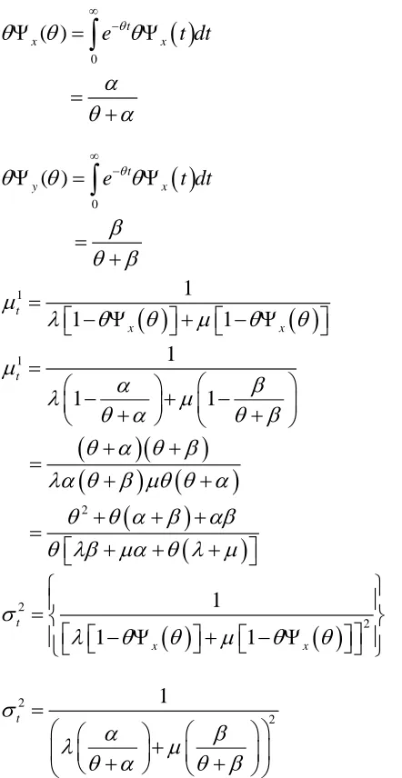
If X_𝑖𝑖𝑠𝑠 and Y_𝑦𝑦𝑠𝑠 are assumed to be exponential with parameter

α

and

β

( )

0

( )

t

x

e

x

t dt

θ

θ

_Ψ

θ

₌

∞ −

θ

_Ψ

∫

α

θ α

=

+

( )

0

( )

t

y

e

x

t dt

θ

θ

_Ψ

θ

₌

∞ −

θ

_Ψ

∫

β

θ β

=

+

( )

( )

1

1

1

1

t

x x

µ

λ

θ

θ

µ

θ

θ

=

− Ψ

+

− Ψ

















1

1

1

1

t

µ

α

β

λ

µ

θ α

θ β

=







₋



₊

₋



₊





₊











(

)(

)

(

θ α θ β

) (

)

λα θ β µθ θ α

+

+

=

+

+

(

)

(

)

2

θ

θ α β

αβ

θ λβ µα θ λ µ

+

+

+

=

+

+

+









( )

( )

2

2

1

1

1

t

x x

σ

λ

θ

θ

µ

θ

θ









= 







− Ψ



+



− Ψ







_

_

_

_

_

_







2

2

1

t

σ

α

β

λ

µ

θ α

θ β

=





_{ +}











_

₊



_



₊













f θ, α and β are kept fixed. Then λ or μ or both increase then mean decreases. Which implies that as the frequency of sexual

contacts or events of needle sharing or both increase then the mean time to seroconversion corresponding graphs are in Fig 1.1a to 1.3, and the corresponding graphs are in Fig. 1.1 a to 1.3 b.

Table-1.1 a: Mean (α =0.5, β = 0.5, θ = 1)

λ μ=1 μ=3 μ=5 μ=7 μ=9

1 0.75 0.375 0.25 0.1875 0.15

2 0.5 0.3 0.2142 0.1666 0.1363

3 0.375 0.25 0.1875 0.15 0.125

4 0.3 0.2142 0.1666 0.1363 0.1153

5 0.25 0.1875 0.15 0.125 0.1071

6 0.2142 0.1666 0.1363 0.1153 0.1

7 0.1875 0.15 0.125 0.1071 0.0938

8 0.1666 0.1363 0.1153 0.1 0.0882

9 0.15 0.125 0.1071 0.0938 0.0833

Table-1.1 b: Mean (α =0.5, β = 0.5, θ = 1)

λ μ=1 μ=3 μ=5 μ=7 μ=9

1 0.5625 0.1406 0.0625 0.0351 0.0225

2 0.25 0.09 0.0459 0.0277 0.0186

3 0.1406 0.0625 0.0351 0.0225 0.0156

4 0.09 0.0459 0.0277 0.0186 0.0133

5 0.0625 0.0351 0.0225 0.0156 0.0115 6 0.0459 0.0277 0.0186 0.0133 0.01 7 0.0351 0.0225 0.0156 0.0115 0.0088

8 0.0277 0.0186 0.0133 0.01 0.0078

Table-1.2 a: Mean (α =0.5, β = 0.5, θ = 1)

μ λ =1 λ =3 λ =5 λ =7 λ =9

1 0.5833 0.2917 0.1944 0.1458 0.1167 2 0.3889 0.2333 0.1667 0.1296 0.106 3 0.2917 0.1944 0.1458 0.1167 0.0972 4 0.2333 0.1667 0.1296 0.106 0.0897 5 0.1944 0.1458 0.1167 0.0972 0.0833 6 0.1667 0.1296 0.106 0.0897 0.0777 7 0.1458 0.1167 0.0972 0.0833 0.0729 8 0.1296 0.106 0.0897 0.0777 0.0686 9 0.1167 0.0972 0.0833 0.0729 0.0648 10 0.106 0.0897 0.0777 0.0686 0.0614

Table-1.2 b: Mean (α =0.5, β = 0.5, θ = 1)

μ λ=1 λ=3 λ=5 λ=7 λ=9

1 0.3402 0.0851 0.0378 0.0212 0.0136 2 0.1512 0.0544 0.0277 0.0168 0.0112 3 0.0851 0.0378 0.0212 0.0136 0.0094 4 0.0544 0.0277 0.0168 0.0112 0.008 5 0.0378 0.0212 0.0136 0.0094 0.0069

6 0.0277 0.0168 0.0112 0.008 0.006

7 0.0212 0.0136 0.0094 0.0069 0.0053

8 0.0168 0.0112 0.008 0.006 0.0047

Table-1.3: (α = 0.5, β = 0.5)

Θ = 1 Θ = 3 Θ = 5 Θ = 7 Θ = 9

λ μ Mean Variance Mean Variance Mean Variance Mean Variance Mean Variance

1 1 0.75 0.5625 0.5833 0.3402 0.55 0.3025 0.5357 0.2869 0.5278 0.2785

2 2 0.375 0.1406 0.2916 0.085 0.275 0.0756 0.2679 0.0717 0.2639 0.0696

3 3 0.25 0.0625 0.1944 0.0378 0.1833 0.0336 0.1786 0.0318 0.1759 0.0309

4 4 0.1875 0.0352 0.1458 0.0212 0.1375 0.0189 0.1339 0.0179 0.1319 0.0174

5 5 0.15 0.0225 0.1166 0.0136 0.11 0.0121 0.1071 0.0115 0.1056 0.0111

6 6 0.125 0.0156 0.0972 0.0094 0.0917 0.0084 0.0893 0.0079 0.0879 0.0077

7 7 0.1071 0.0115 0.0833 0.0069 0.0786 0.0061 0.0765 0.0058 0.0754 0.0057

8 8 0.0937 0.0088 0.0729 0.0053 0.0688 0.0047 0.0665 0.0045 0.0659 0.0044

REFERENCES

1. Ahlgren, D.J. Stein, A.C., and Lyons, P.A. (1987) Computers model of the AIDS Epidemic Arch. AIDS Research 1, 69-79.

2. Anderson, R.M. (1988). The Epidemiology of HIV infection variable incubation plus infectious periods and heterogeneity in sexual activity. Journal of Royal Statistical Society. 151, 66-93.

3. Esary, J. D., Marshall, A. W. and Proschan, F. (1973). Shock models and Wear processes, Ann. Probability, 1(4): 627-649.

4. Nowak, M.A. and May, R.M. (1991). Mathematical Biology of HIV Infections Antigenic Variation and Diversity Threshold, Mathematical Biosciences, Vol.106:1-21.

5. Stilianakis, N. Schenezele, D and Dietz, K. (1994). On the antigenic diversity threshold model for AIDS. Mathematical Biosciences, Vol: 121, 235-247.

6. S.C. Premila and Dr. S. Srinivasa Ragavan (May 2014) A Stochastic Model for time to cross Antigenic Diversity Threshold of HIV infection under Preventive Strategy. International Journal of Mathematical Archive – 5(5), 129-134.

Source of support: Nil, Conflict of interest: None Declared