Temporal Stability of Trip Generation Models: An Investigation of the Role of Model Type and Life Cycle, Area Type, and Accessibility Variables.

(1)

ABSTRACT

HUNTSINGER, LETA FAY. Temporal Stability of Trip Generation Models: An Investigation of the Role of Model Type and Life Cycle, Area Type, and Accessibility Variables. (Under the direction of Nagui M. Rouphail.)

Transportation plays a significant role in the mobility, economic health, and quality of life of our communities. The transportation planning process is a complex process of developing and evaluating strategies to meet an area’s long-term goals. Planning is inherently a public process that connects us to the future. In the field of transportation planning, travel demand models are often the tool used to make this connection. Travel demand models forecast future travel demand based on forecast input variables related to land use and demographic factors. A fundamental assumption of travel demand models is that model parameters remain stable over time. A violation of this assumption could lead to transportation analyses and travel forecasts that either over- or underestimate travel demand and associated transportation deficiencies, which could in turn lead to poorly allocated investments in transportation infrastructure. Developing a better understanding of the factors that influence travel behavior, the changes in travel behavior over time, and the explanatory variables that best capture these changes may lead to the development of models that are more temporally stable.

(2)

The findings from this analysis show that both the generation choice and cumulative logistic regression models are good models for trip generation. There is also evidence of temporal stability for these two models, perhaps even better than the more widely used cross-classification model based on findings reported in the literature. The introduction of explanatory variables defining life cycle, area type, and accessibility do not noticeably improve model fit, but there is evidence of improved model verification and temporal stability. Finally, analysis shows that trip rates that change over time can have implications for systems and project level planning, resulting in unexpected changes in vehicle miles traveled and associated emissions, transit ridership, traffic forecasts, and localized travel.

(3)

(4)

Temporal Stability of Trip Generation Models: An Investigation of the Role of Model Type and Life Cycle, Area Type, and Accessibility Variables

by

Leta Fay Huntsinger

A dissertation submitted to the Graduate Faculty of North Carolina State University

in partial fulfillment of the requirements for the degree of

Doctor of Philosophy

Civil Engineering

Raleigh, North Carolina 2012

APPROVED BY:

_______________________________ ______________________________

Dr. Nagui Rouphail, Chair Dr. John Stone

________________________________ ________________________________

(5)

DEDICATION

(6)

BIOGRAPHY

(7)

talented (and fun!) travel modelers in the country. Leta entered the doctoral program in Civil Engineering at NCSU in 2009 under the direction of Dr. Nagui Rouphail. During her years in the program, she worked part time with the Durham-Chapel Hill-Carrboro Metropolitan Planning Organization as the team leader for technical services.

(8)

ACKNOWLEDGMENTS

From dream, to concept, to completion, I did not undertake this effort without the influence, support, and guidance of mentors, professors, family, and friends. I have been blessed to have many mentors who have guided me along my journey. The first of these is John Bauerlein, former Traffic Engineer for the City of Wilmington, my first manager and mentor. John made me believe that I could do anything and put into place a support system to make it so. Over the course of my career, I have tried to emulate the things he taught me with those that I have been fortunate to lead and work with. Next along my path, I must acknowledge Dr. M.R. (Ron) Poole, the father of transportation planning in North Carolina. Ron saw in me a passion for learning and encouraged me to pursue my Ph.D. Even after a couple of false starts, Ron was always persistent, but never pushy, in encouraging me not to give up on my goal or my dream. Blake Norwood, former manager of the Transportation Planning Branch taught me courage and the power and payoff of teamwork. Blake fed my curiosity and thirst for knowledge by giving me challenging and interesting projects. I also want to thank Dr. Rick Donnelly for this friendship and support. While my pursuit for higher education did not afford me the opportunity to work with Rick for long, I value tremendously the time we spent together and the things he taught me that go beyond technical knowledge. I especially want to thank him for the time he invested in reading my research proposal, and for the advice he gave that made it stronger. Finally, I want to thank my committee chair, Dr. Nagui Rouphail for his support and guidance in the completion of my dissertation. My decision to finally commit to finishing my PhD is in large part due to his encouragement. Words cannot express my gratitude. All of these individuals have contributed to where I am today through their guidance, insights, accessibility, support, and respect.

(9)

advisor to friend. I have enjoyed the time we have spent working on research projects together, co-instructing CE 701, and discussing life beyond the 8 to 5. Thank you for your friendship and support over the years. I also want to thank Dr. Peter Bloomfield for the assistance he provided on the statistics and model estimation work.

(10)

TABLE OF CONTENTS

LIST OF TABLES ... xiv

LIST OF FIGURES ... xvii

CHAPTER 1. INTRODUCTION ... 1

1.1 Research Need ... 1

1.2 Research Objectives ... 1

1.3 Trip Generation Models – State of the Practice ... 2

1.4 Motivation ... 4

1.5 Approach ... 6

1.5.1 Phase 1: Data Analysis Approach ... 6

1.5.2 Phase 2: Model Development Approach ... 7

1.5.3 Phase 3: Comparative Analysis Approach ... 8

1.5.4 Phase 4: Case Study Approach ... 8

1.6 Significance of the Research ... 9

1.7 Research Scope and Limitations ... 9

1.8 Dissertation Organization ... 10

CHAPTER 2. DATA DESCRIPTION ... 11

2.1 Introduction ... 11

2.2 Baltimore Metropolitan Commission Data ... 12

2.3 Research Triangle Region Data ... 14

2.4 Cleaning and Processing Data for the Baltimore Region ... 17

2.5 Cleaning and Processing Data for the Triangle Region ... 18

(11)

2.5.2 Assigned Travel Days - Weekly versus Weekdays Only ... 19

2.5.3 Household Members Age 5 and Older versus All Household Members ... 19

2.5.4 Differences in geographic coverage ... 19

2.5.5 Under-sampling of Durham County ... 19

CHAPTER 3. URBAN TRENDS AND CHANGES IN TRIP MAKING ... 21

3.1 Introduction and Motivation ... 21

3.2 Literature Review... 21

3.3 Methodology ... 23

3.3.1 Data Collection ... 23

3.3.2 Data Preparation... 25

3.3.3 Data Analysis ... 26

3.4 Results ... 28

3.4.1 Demographic and Urban Change ... 28

3.4.2 Trip Rates ... 30

3.4.3 Comparisons with NHTS ... 35

3.5 Summary of Findings ... 36

3.6 Conclusions and Recommendations ... 41

CHAPTER 4. INFLUENCE OF LIFE CYCLE ... 42

4.3 Data Description ... 45

(12)

4.5.1 Life Cycle and Travel Behavior ... 51

4.5.2 Life Cycle and Temporal Effects ... 52

4.6 Analysis and Results ... 53

4.6.1 Life Cycle and Travel Behavior ... 53

4.6.2 Life Cycle and Temporal Effects ... 59

4.7 Summary and Recommendations ... 62

CHAPTER 5. INFLUENCE OF AREA TYPE AND ACCESSIBILITY ... 65

5.2.1 Accessibility ... 66

5.2.2 Area Type... 67

5.3.1 Data ... 68

5.3.2 Statistical Tests ... 69

5.4 Accessibility Definitions ... 71

5.5 Area Type Definitions... 74

5.6.1 Accessibility, Area Type and Travel Behavior ... 76

5.6.2 Temporal Effects ... 82

5.7 Summary and Conclusions ... 83

CHAPTER 6. GENERATION CHOICE MODELS ... 87

(13)

6.2.1 Trip Generation Models ... 88

6.2.2 Transferability ... 89

6.3.1 Data ... 91

6.3.2 List of Variables ... 91

6.3.3 Model Estimation ... 94

6.3.4 Tests of Temporal Stability ... 95

6.4.1 Model Specification ... 98

6.4.2 Model Estimation Results ... 98

6.4.3 Temporal Stability ... 103

CHAPTER 7. CUMULATIVE LOGISTIC REGRESSION MODELS... 111

7.2.1 Trip Generation Models ... 112

7.3.1 Data ... 114

7.3.2 List of Variables ... 115

7.3.3 Cumulative Logistic Regression Model ... 118

(14)

7.4.1 Model Specification ... 122

7.4.2 Model Estimation Results ... 122

7.4.3 Model Verification ... 126

7.4.5 Backwards Temporal Stability ... 134

CHAPTER 8. ASSESSING THE IMPACT OF SAMPLE SIZE, MODEL TYPE, AND EXPLANATORY VARIABLES ON TEMPORAL STABILITY... 141

8.2.1 Survey Data and Variable Description ... 142

8.2.2 Model Estimation and Verification ... 145

8.2.4 Experimental Design ... 149

8.3 Results ... 150

8.3.1 Generation Choice ... 150

8.3.2 Cumulative Logistic Regression ... 156

8.4 Comparative Analysis ... 160

8.4.1 Model Performance ... 160

8.5 Findings and Recommendations ... 164

8.5.1 Model Performance Findings ... 164

8.5.2 Temporal Stability Findings ... 164

(15)

CHAPTER 9. EVALUATING THE IMPLICATIONS OF TEMPORAL INSTABILITY . 166

9.3 Study Methodology ... 168

9.3.1 Case Study 1 - Research Triangle Region, North Carolina ... 169

9.3.2 Case Study 2 - Jackson County, North Carolina ... 170

9.3.4 Trip Rate Development ... 170

9.3.5 Trip Generation Performance Measures ... 172

9.3.6 System Level Performance Measures ... 172

9.3.7 Key Project Performance Measures ... 173

9.4.1 Research Triangle Region, NC ... 173

9.4.2 Jackson County, NC... 177

9.4.3 Implications of Temporal Instability over the Longer Term ... 180

9.5 Summary of Findings ... 182

9.6 Conclusions and Recommendations ... 184

CHAPTER 10. SUMMARY, FINDINGS AND RECOMMENDATIONS ... 185

10.1 Summary ... 185

10.1.1 Phase 1: Data Analysis... 185

10.1.2 Phase 2: Model Development ... 186

10.1.3 Phase 3: Comparative Analysis ... 186

(16)

10.2.1 Phase 1: Data Analysis... 187

10.2.2 Phase 2: Model Development ... 188

10.2.3 Phase 3: Comparative Analysis ... 188

10.2.4 Phase 4: Case Studies... 189

10.3 Recommendations for Professional Practice ... 190

10.4 Recommendations for Future Research ... 191

REFERENCES ... 193

APPENDIX ... 201

APPENDIX A: EXAMPLE BIOGEME OUTPUT ... 202

(17)

LIST OF TABLES

Table 1. Baltimore Region Trip Statistics ... 33

Table 2. Triangle Region Trip Statistics ... 34

Table 3. NHTS Trip Rate Statistics ... 35

Table 4. Percent Change for NHTS Trip Rate Statistics ... 36

Table 5. NHTS Life Cycle Definition ... 47

Table 6. Kermanshah Life Cycle Definition ... 47

Table 7. Sun Life Cycle Definition ... 48

Table 8. Marker Life Cycle Definition ... 49

Table 9. Vadarevu Life Cycle Definition ... 50

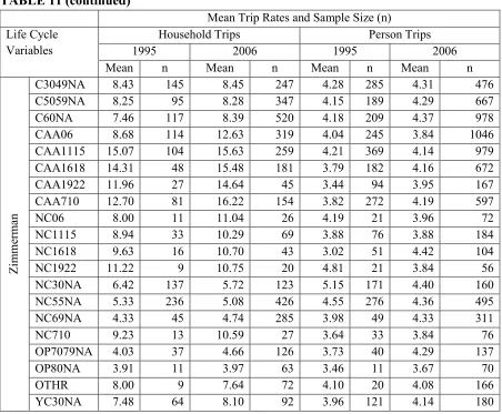
Table 10. Zimmerman Life Cycle Definition ... 50

Table 11. Household and Person Mean Trip Rates and Sample Size (n) by Life Cycle ... 53

Table 12. Calculated p-value and eta-square (η2_{) for Life Cycle Mean Trip Rates}_{... 57}

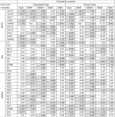
Table 13. NHTS Variable-to-Variable Comparisons using 2006 Household Trip Rate ... 58

Table 14. Number and Percent of Cells Showing a Significant Difference in Mean Trip Rate for Variable-to-Variable Comparisons by Life Cycle Definition ... 59

Table 15. Life Cycle Mean Trip Rate Temporal Analysis between 1995 and 2006 ... 61

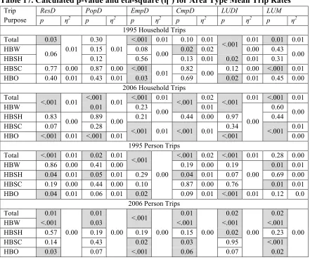
Table 16. Calculated p-value and eta-square (η2_{) for Accessibility Mean Trip Rates}_{... 77}

Table 17. Calculated p-value and eta-square (η2_{) for Area Type Mean Trip Rates}_{... 78}

Table 18. Final Stratifications for Area Type and Accessibility Definitions ... 80

Table 19. Household and Person Mean Trip Rates and Sample Size (n) ... 81

Table 20. Results of Mean Trip Rate Temporal Analysis between 1995 and 2006 ... 83

Table 21. Model Estimation Results for Case 1 Models ... 101

Table 22. Model Estimation Results for Case 2 Models ... 102

(18)

Table 25. Model Estimation Results for HBW Case 1 Models Using 1995 Survey ... 123

Table 26. Model Estimation Results for HBO Case 1 Models Using 1995 Survey ... 124

Table 29. Model Verification Measures for Models Estimated Using 1995 Survey ... 127

Table 34. Measures of Temporal Stability for 1995 Case 1 Models Applied to 2006 Socio-economic Data ... 132

Table 35. Measures of Temporal Stability for 1995 Case 2 Models Applied to 2006 Socio-economic Data ... 134

Table 36. Model Estimation Results for HBW and HBO Case 3 and Case 4 Models using 2006 Survey ... 135

Table 37. Model Verification Measures for Models Estimated Using 2006 Survey ... 136

Table 38. Measures of Temporal Stability for 2006 Models Applied to 1995 Socio-economic Data ... 137

Table 39. Generation Choice HBW Worker Model Estimation Results ... 151

Table 40. Generation Choice HBO Worker Model Estimation Results ... 152

Table 41. Generation Choice HBO Non-Working Adult Model Estimation Results ... 153

Table 42. Generation Choice HBO Child Model Estimation Results ... 153

Table 43. Model Verification Measures for Generation Choice Models ... 154

Table 44. Measures of Temporal Stability for Estimated Generation Choice Models Applied to Socio-economic Data ... 156

Table 45. Model Estimation Results for HBW Models using 1995 and 2006 Survey ... 157

Table 46. Model Estimation Results for HBO Models using 1995 and 2006 Survey ... 158

(19)

Table 48. Measures of Temporal Stability for Estimated Cumulative Logistic Regression

Models Applied to Socio-economic Data ... 160

Table 49. Percent Change in Trip Rates by Trip Purpose... 171

Table 50. Typical Ranges for Trip Generation Performance Measures ... 172

Table 51. Typical Ranges for VMT Performance Measures ... 173

Table 52. Generalized Annual Average Daily Volumes by Level of Service (LOS) ... 173

Table 53. TRM Performance Measures ... 177

Table 54. Jackson County Performance Measures ... 180

(20)

LIST OF FIGURES

Figure 1. Research Phases... 6

Figure 2. Baltimore Survey Boundaries... 14

Figure 3. Triangle Survey Boundaries ... 16

Figure 4. Percent Change in Trips per Household ... 37

Figure 5. Percent Change in Trips per Person ... 38

Figure 6. Percent Change in Regional Census Demographics ... 39

Figure 7. Triangle Survey Boundaries ... 69

Figure 8. Experimental Design ... 150

Figure 9. Percent Change in Trip Rates by Trip Purpose and Rate Set ... 171

Figure 10. TRM Percent Trips by Trip Purpose by Trip Rate Set ... 175

Figure 11. TRM Project Demand by TR Set and Level of Service ... 176

Figure 12. Jackson Percent Trips by Trip Purpose by Trip Rate Set ... 178

(21)

CHAPTER 1. INTRODUCTION

Transportation plays a significant role in the mobility, economic health, and quality of life of our communities. It shapes growth by providing access to land and shapes public policy in areas related to “air quality, environmental resource consumption, social equality, land use, urban growth, economic development safety, and security” (FHWA 2007). The transportation planning process is a complex process of “developing strategies for operating, managing, maintaining, and financing an area’s transportation system in such a way as to advance the area’s long-term goals” (FHWA 2007). Planning is inherently a public process that connects us to the future. In the field of transportation planning, this connection to the future is often made through the development and application of travel demand models that are used to forecast future demand in travel based on forecast input variables related to land use, demographics, and socio-economic factors. Primary among the steps of a travel demand model is that for trip generation, the topic of this research. If the trip generation sub-model is inaccurate, the results of subsequent steps (trip distribution, mode choice and trip assignment) will be wrong.

1.1 Research Need

A peer exchange held in December 2004 to discuss issues of data transferability identified temporal transferability (stability) as a concept that is regularly assumed by modelers, while the validity of this concept has not be sufficiently studied (TMIP 2004). Without a better understanding of temporal stability, it is difficult to defend the use of model parameters developed in one point in time to forecast behavior many years into the future. This research adds to that understanding for trip generation models, and addresses the question of whether survey sample size, model form, and explanatory variables defining life cycle, area type, and accessibility contribute to temporal stability.

(22)

tested is that advanced models such as the generation choice and cumulative logistic regression models are temporally stable, and that the temporal stability of these models improves with the inclusion of key explanatory variables such as lifecycle, area type, and accessibility. Lifecycle can be defined in a number of different ways, but is generally used to describe changes that people undergo from infancy, to childhood, to adulthood, to old age as a means of better understanding how these various cycles influence travel behavior (Zimmerman 1981). Area type describes land use and development type with respect to population and employment, while accessibility captures characteristics of the supply side of the transportation system. These are conceptual definitions; this research will explore and recommend definitions that seek to improve the explanatory power and temporal stability of trip generation rates and parameters.

The specific objectives of this research are to:

1. Better understand changes in travel behavior and the factors that influence travel behavior over time, especially with respect to lifecycle, accessibility, and area type; 2. Evaluate the usefulness of a new family of discrete choice models for trip generation; 3. Provide insights into the temporal stability of discrete choice trip generation models; 4. Compare the models estimated with and without lifecycle, accessibility, and area type

variables to determine whether these variables improve temporal stability of trip generation rates; and

5. Conduct two case studies to evaluate the implication of trip rates that do not remain stable over time.

1.3 Trip Generation Models – State of the Practice

(23)

model provides an estimate of the number of trips generated and attracted to each traffic analysis zone (TAZ) in the study area.

Trip generation models have taken many forms over the years, including zonal regression models, household regression models, and cross-classification models. Early travel forecasts consisted primarily of the extrapolation of “desire lines” developed from origin-destination (OD) surveys (FHWA 1975). This practice advanced in the early 1950s to consider land use and socio-economic factors in quantifying urban trip volumes, providing an analytical approach for using future land use plans to estimate future travel demand (FHWA 1975). Regression models of trip generation became commonplace in the late 1950s and early 1960s opening the door for a greater insight into travel and the factors influencing it (FHWA 1975). Regression models have the advantage of allowing the analyst to consider multiple independent variables, but the disadvantage of treating trip rates as continuous rather than discrete.

The 1970s marked a shift away from aggregate zonal level regression analysis to disaggregate household cross-classification procedures. Cross-classification models estimate an average number of trips as a function of two or more household attributes (Ortuzar and Willumsen 2011). This method has long been the most established model for estimating trips in a travel demand model. Cross-classification models overcome the limitations of regression models, but introduce another shortcoming with respect to the number of variables and stratifications considered before violating the minimum sample size requirements (about 30 samples per stratification), or conversely making the survey sample size prohibitively expensive. Another disadvantage of cross-classification is the lack of goodness of fit measures.

(24)

used for mode choice modeling, recent applications have also considered destination choice, and even more recently generation choice. Generation choice models estimate the frequency of daily person trips. Models that estimate person trips are an improvement over household based models as they allow for a greater use of important variables and are more compatible with other components of the modeling system (Ortuzar and Willumsen 2011).

In addition to choice-based models, another form of disaggregate model for trip generation is the cumulative logistic regression model. Cumulative logistic regression models, also known as ordered logistic regression, estimate relationships between an ordered categorical dependent variable and a set of independent variables.

Generation choice and cumulative logistic regression models offer several advantages over the commonly used cross-classification model, including the flexibility to consider more independent variables, the ability to include continuous variables in addition to classification variables, and statistical measures for evaluating the significance of the independent variables. Also, unlike the cross-classification model, where sample size quickly limits the number of explanatory variables due to the requirement that any given cell have at least 30 observations, a disaggregate model can capture multiple explanatory variables, making it possible to capture relationships that are not possible with the standard cross-classification approach (PB 2007).

1.4 Motivation

(25)

analyses and travel forecasts that either over- or underestimate travel demand and associated transportation deficiencies, which could in turn lead to poorly allocated investments in transportation infrastructure.

Trip generation models are the first in the sequence of models used to forecast travel demand. As the first step in the model chain, forecasting errors in this step may compound errors in the remaining steps. An initial goal of these models is to represent observed travel behavior, but that is only part of the challenge. These models must also forecast future travel behavior based on a set of assumed future input demographics (land use and population scenarios) and the travel behavior relationships captured in the model specification. The second goal may be as important as the first since travel demand models play a significant role in the transportation planning process, providing transportation planners, highway designers, transit operators, and decision makers with critical data needed for the development and implementation of transportation plans, projects and policies.

Poor forecasts can be the result of many things including errors in model specification, model calibration, model verification, and input data. Forecasting error can also result from model parameters that change over time, or in other words, when the behavior captured by the base year parameters does not hold true in the future. Trip generation rates (parameters) that change over time could lead to traffic forecasts that result in over designing and building transportation projects, further leading to overspending limited public resources. In the case of revenue generating projects, such as a toll road, forecasts higher than those eventually observed could lead to revenue collections that are lower than anticipated, leading to financial challenges over the life of the project and loss of public confidence.

(26)

techniques can improve the quality of the input data. Improving our understanding of the factors that influence travel behavior and how these factors change over time can lead to better temporal stability of travel models.

The purpose of this research is to investigate changes in trip rates over time in order to develop a better understanding of these changes and the factors that influence these rates. The question considered in this investigation is whether certain variables related to households and individuals provide greater insight into temporal stability of trip generation models.

1.5 Approach

The research is conducted in four phases 1) data analysis, 2) model development, 3) comparative analysis, and 4) case studies, see Figure 1.

Figure 1. Research Phases

The data analysis phase is conducted in two parts: 1.5.1 Phase 1: Data Analysis Approach

(27)

2. An investigation of multiple definitions for life cycle, area type, and accessibility in order to assess the value of each in explaining trip making behavior between strata, trip purpose, and across time.

The comparison of trip rates uses both the Baltimore and Triangle datasets. The examination includes the percent change across time for various demographic and travel statistics as well as the t-statistic to test the null hypothesis of no significant difference between trip rates. The investigation of life cycle, area type, and accessibility is limited to survey data from the Triangle region, as supplemental data needed to calculate the variables for life cycle, area type and accessibility is not available for the Baltimore region. The research explores definitions of life cycle, area type, and accessibility documented in previous research. This included six definitions for life cycle, six different methods for assessing area type, and 24 accessibility definitions. ANOVA is used to evaluate the performance of the various definitions in explaining differences in travel behavior.

Using the findings from Phase 1, generation choice and cumulative logistic regression models for home-based work (HBW) and home-based other (HBO) trips are estimated first considering explanatory variables widely used in trip generation models, and second supplementing these variables with the variables from Phase 1 defining life cycle, area type, and accessibility.

1.5.2 Phase 2: Model Development Approach

(28)

Model performance is assessed through an examination of model verification statistics including person trips per person, person trips per household, HBW trips per worker, and a comparison of estimated to observed total trips for both trip purposes.

The measures of temporal stability include:

1. How well the models estimated in one year predict total trips by trip purpose observed in another year;

2. How well the models estimated in one year predict the fractions of trips by trip purpose and stratification observed in another year;

3. How well the individual model parameters compare between years; and

4. How well the overall contribution of the model parameters compares between years.

The Phase 3 approach is similar to Phase 2, but whereas Phase 2 focused on models estimated using 1995 survey data applied in the 2006 context, Phase 3 expanded the analysis to include models estimated using 2006 survey data applied in the 1995 context. This second round of model development allows for a detailed comparison of the models exploring sample size, model form, and temporal stability.

1.5.3 Phase 3: Comparative Analysis Approach

The case study analysis involves a series of model runs using two different case studies. The first case study considers a regional travel demand model and the second a traditional trip based travel demand model for a small urban area. The first model run is the baseline model and reflects the original trip rates for the validated model. Subsequent model runs include one model run for each of three trip rate sets based on the Baltimore and Triangle surveys, and then a fourth trip rate set capturing changes observed between the 1977 and 2001 National Household Travel Survey (NHTS). Trip generation, system level, and project performance measures quantify the effect of the rate changes on the model results.

(29)

1.6 Significance of the Research

This research provides important information for travel model developers and contributes to the conversation on the temporal stability of trip generation models. As noted earlier, an underlying assumption of trip generation models is temporal stability, but little information exists on modeling techniques or explanatory variables that support temporal stability. This research explores three such explanatory variables and makes recommendations on their definition and application. This research also explores two modeling techniques for trip generation and makes recommendations regarding application and temporal stability. The findings outlined in this research support the development of advanced trip generation models. In this context, advanced trip generation models refer to discrete choice models where trip generation is the selection of one trip alternative from among a set of mutually exclusive trip alternatives. This research also informs the debate on whether it is worth the additional expenditure of time and resources to develop advanced models.

1.7 Research Scope and Limitations

The scope of this research focuses on data analysis and the development of advanced trip generation models. The focus of the data analysis is on gaining a better understanding of trip making behavior, changes in trip making behavior over time, and the factors that contribute to these changes. Model development provides insights into the role that model type and explanatory variables defining life cycle, area type, and accessibility have on temporal stability. Three household travel surveys from Baltimore, Maryland, administered in 1977, 1993, and 2001, and two from the Research Triangle region of North Carolina administered in 1995 and 2006 form the basis of the data analysis tasks. The 1995 and 2006 Triangle surveys supplemented with supporting land use and transportation network data form the basis of the model development tasks.

(30)

choice and cumulative logistic regression models and is limited to two datasets for one geographic region approximately ten years apart.

1.8 Dissertation Organization

(31)

CHAPTER 2. DATA DESCRIPTION

The data sets supporting this research include five household travel surveys from five different points in time. Three surveys are from the Baltimore Metropolitan Region, Maryland, and two are from the Research Triangle Region, North Carolina. This chapter describes the various data sets and the cleaning and processing necessary to prepare the data for analysis.

2.1 Introduction

The ideal datasets for this research would be household travel surveys collected at two or more different points in time, covering the same geographic region, using the same survey methodology, and covering a period of at least 20 years. In order to test key factors such as lifecycle, area type, and accessibility and to test the application of the estimated models supporting census data, socio-economic and demographic data, traffic analysis zones, and transportation networks for each period is also required. Unfortunately, several factors contribute to the difficulty in identifying such data, including changes in survey methodology and changes in modeling technology.

(32)

software to GIS based modeling software. Command line software greatly limited the number of attributes coded to describe the transportation system as well as the true spatial representation of the transportation system. These differences would likely influence the calculation of accessibility variables. Perhaps the biggest impediment to finding these ideal datasets is that few agencies saw the benefit of archiving all the development elements of historic data and model sets.

The previously listed factors present a challenge for the investigation of temporal stability, given that most travel demand models are used to forecast travel 20 to 30 years out. One could argue that changes measured within the first 10 years of model application are far less radical than changes 20 to 30 years out. However, with few datasets spanning 20 to 30 years, the ability to analyze temporal changes was limited in this research. The research overcomes the dataset limitation through the implementation of the two-tiered approach that uses datasets from two different urban areas as discussed below.

The key datasets supporting this research are the 1977 Baltimore Travel Data (Harvey 1980), the 1993 Baltimore Travel Data (Minnesota 2010), the 2001 Household Travel Survey: Baltimore Region Analysis (BMC 2005), the 1994/1995 Triangle Travel Behavior Survey (NuStats 1995), and the 2006 Greater Triangle Travel Survey (NuStats 2006).

2.2 Baltimore Metropolitan Commission Data

(33)

for key variables in the 1993 survey. Baltimore datasets for 1977, 1993, and 2001 include household, person, and trip data for each year. The availability of raw data from 1977, 1993, and 2001 and documentation from 1977 and 2001 is one of the key reasons survey data for the Baltimore region was selected for this analysis. A prior working relationship with staff at BMC and familiarity with the region was a secondary reason for selecting the BMC data.

(34)

Figure 2. Baltimore Survey Boundaries

The Baltimore region has likely experienced significant growth and urbanization between 1977 and 2001. To understand changes and the possible affect on travel behavior, this research will include not only an analysis of the survey data, but also of available census and demographic data.

2.3 Research Triangle Region Data

(35)

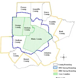
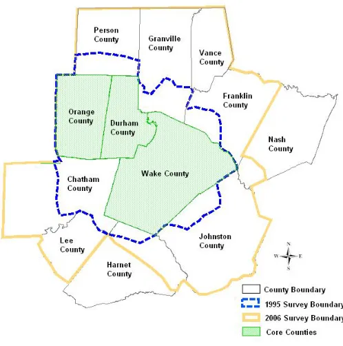
The 1995 Triangle Travel Behavior Survey (1995 Survey) covered the period between November 1994 and April 1995 and the North Carolina counties of Wake, Durham, Orange and portions of Harnett, Chatham, Person, Granville, Franklin, and Johnston. See Figure 3. The 1995 Survey was an activity-based survey, favored over a more traditional trip-based survey because it leads to a better understanding of travel as a “derived demand” and places travel within the context of activities that the traveler participates in over the course of the day (NuStats 1995). The sample was a stratified random sample that included 1,778 households. Stratification reflected geographic location defined as urban (greater than 1,920 households per square mile), suburban (133 – 1,920 households per square mile), and rural (zero – 133 households per square mile). The 1995 Survey collected activity and travel data for all household members five and older over a 48-hour period; travel days covered weekday and weekend travel. The 1990 Census STF-3A data file formed the universe for the survey sample. Data files include household characteristics, person characteristics, activities, and vehicles.

(36)

Figure 3. Triangle Survey Boundaries

While both surveys used CATI technology, several other methodological differences exist between the 1995 and 2006 datasets as summarized below; Section 2.5 provides a recommended approach for addressing, as necessary, these differences.

1. The 1995 48-hour survey versus the 2006 24-hour survey

2. The 1995 survey was a 7-day survey versus weekdays only for the 2006 survey 3. Household members age 5 and older were sampled in the 2006 survey as compared to

all household members in the 1995 survey

4. The 2006 survey covered a larger geographic region

(37)

There are several advantages of using these two datasets to answer the proposed research question regarding temporal stability of trip generation rates. The first noted advantage is that the datasets are easily available and already familiar to me. A second and more important advantage is that both surveys are activity-based surveys of person trips collected by the same survey firm using CATI technology. The activity-based surveys should minimize response differences that might result from different survey instruments or techniques. Recording person trips instead of vehicle trips supports the estimation of person based generation choice models. As previously noted, the surveys cover an eleven-year period, which capture the typical 10-year time horizon when most agencies undertake a major data collection and travel model update exercise. Both surveys include the geographic region of interest and have the added advantage of corresponding with a geographic region that includes secondary supportive data as outlined below.

Secondary data that will support this research include highway networks from 1995 and 2006, socio-economic data from 1995 and 2006, and 1990 and 2000 decennial census data including SF3 and Census Transportation Planning Package (CTPP) data. All data are readily available from the Capital Area Metropolitan Planning Organization (CAMPO), the Durham-Chapel Hill-Carrboro MPO (DCHC MPO), and the Triangle Regional Model Service Bureau (TRMSB). As with the Baltimore region, data analysis includes census and other demographic data to understand factors influencing urban trends and changes in travel behavior.

2.4 Cleaning and Processing Data for the Baltimore Region

(38)

home-based trips (NHB). The development and application of a consistent definition for each trip purpose helped assure that changes noted in the data analysis are not the result of using different definitions of trip purpose. This process was somewhat more limited than the one applied to the Triangle region (described below) due to limited familiarity with, and details within the data. Generation of a person trip file consisted of appending trip data from the trip record file to the person record file. Data processing included the generation of additional variables such as worker status, household size, income group, vehicle ownership group, household workers, and household children for the purposes of facilitating the reporting of statistics. The aggregation of trip records for each individual within a given household produced the household trip file. The final processing step involved flagging weekend travel records in order to exclude them from the analysis. Reasonableness checks of the data included the creation and review of various summaries of the survey data.

2.5 Cleaning and Processing Data for the Triangle Region

Section 2.3 noted several methodological differences that exist between the 1995 and 2006 datasets; summarized below is the recommended approach for reconciling these differences. The weighting and expansion of both datasets utilized census data by county stratified by household size and vehicles per household. Reasonableness checks using weighted and unweighted data include comparisons against household income, ethnicity, and owner status. Applying this consistent approach to both datasets helps assure that changes noted in the data analysis are not the result of using two different approaches to weighting and expansion.

(39)

The weighting process will use demographic and geographic characteristics, therefore the removal of Saturday and Sunday records will not affect the estimation dataset.

2.5.2 Assigned Travel Days - Weekly versus Weekdays Only

Exclusion of trip records for household members under age 5 from the estimation dataset assures that the datasets match as closely as possible. This will not affect the weighting of the survey records.

2.5.3 Household Members Age 5 and Older versus All Household Members

Both datasets will be re-weighted using a consistent method and geography. New expansion factors will also reflect a consistent method. This process will account for the original differences in geography.

2.5.4 Differences in geographic coverage

The consistent weighting and expansion methodology for both the 1995 and 2006 datasets results in weighting and expansion factors that adjust for the under-sampling of Durham households in the 1995 survey.

2.5.5 Under-sampling of Durham County

The steps to weight and expand the survey data are: 1. Summarize 1990 and 200 census data

2. Remove weekend travel records from the 1996 dataset 3. Remove travel for household members under age 5

4. Remove records for all geographies outside Wake, Durham, and Orange counties 5. Develop new expansion factors

6. Develop new weights

(40)

linked trips. An unlinked trip refers to a very short segment trip that is a part of a traveler’s daily activity but not traditionally considered a separate trip for the purposes of travel demand modeling. An example of two unlinked trips processed to represent one linked trip would be a traveler stopping for fuel on the way to work, which would be coded as one work trip rather than a work-to-other and then other-to-work trip. Identical linking procedures for both surveys will eliminate any differences related to trip definitions. Finally, overall reasonableness checking will investigate, and repair as necessary, coding errors and inconsistencies.

(41)

CHAPTER 3. URBAN TRENDS AND CHANGES IN TRIP MAKING 3.1 Introduction and Motivation

A travel demand model is a series of mathematical equations used to describe travel and travel choices. In its most basic form, this series of models is broken into a 4-step process, trip generation, trip distribution, mode choice, and trip assignment. Best practice models use locally collected travel survey data to estimate and calibrate the models. Planners use these models to forecast travel demand 20 – 30 years into the future for the purposes of evaluating transportation strategies and investment. An implicit assumption of a travel demand model is that model parameters remain stable over time (Ortuzar and Willumsen 2011). A violation of this assumption could lead to transportation analyses and forecasts that over- or underestimate travel demand and associated transportation deficiencies, which could in turn lead to poorly allocated investments in transportation infrastructure.

Understanding how travel behavior changes over time can lead to the development of better models that capture this change within the model specification. The purpose of this paper is to investigate changes in trip rates over time in order to develop a better understanding of these changes and the explanatory variables that influence these rates. The question considered in this investigation is whether certain explanatory variables related to households or individuals provide greater insight into temporal stability of trip rates and if those variables can improve temporal stability if necessary.

3.2 Literature Review

(42)

per household increased from 6.36 to 10.39 (Hu and Reuscher 2004). The biggest change was in person trips per day related to family or personal business. These trips increased from 0.91 in 1977 to 1.79 in 2001, a near doubling of the 1977 rate (Hu and Reuscher 2004). A study on changes in activity participation in the Puget Sound Region also documented an increase in the number of shopping trips taken over time (Yee and Niemeier 2000).

An examination of historical trip rate data clearly shows changes, posing a challenge for travel model developers, as one of the underlying assumptions of these models is that the parameters reflecting the behavior represented by explanatory variables remain stable over time. In this context, an explanatory variable might refer to household size or income, and the parameter the average number of trips for each individual or combination of explanatory variables.

(43)

Other studies have focused on the temporal stability of trip production rates estimated from household survey data. In this context, temporal stability is concerned with how models developed during one period of time transfer to a future period. It also considers how trip rates estimated with data from one period compare to rates estimated with data from a future period. The literature indicates a heavy focus on the temporal stability of travel models during the 1970s (see Ashford, 1972 (Ashford and Holloway 1972); Kannel and Heathington, 1973 (Kannel and Heathington 1973); Smith and Cleveland, 1976 (Smith and Cleveland 1976); Yunker, 1976 (Yunker 1976); Doubleday, 1977 (Doubleday 1977) ), while current work in this area has focused on spatial transferability (see Wilmot, 1995 (Wilmot 1995); Agyemang-Duah and Hall, 1997 (Agyemang-Duah and Hall 1997); Cotrus, 2005 (Cotrus, Prashker et al. 2005); Mohammadian, 2007 (Mohammadian and Zhang 2007); Everett, 2009 (Everett 2009)). The focus on spatial transferability is in response to both the lack of survey data in many urban areas as well as the increased cost for collecting such data (TMIP 2004; Everett 2009). While much remains for exploration in the area of spatial transferability, revisiting the issue of temporal stability is equally important. There are increasing constraints on funds available for infrastructure improvements (TRB 2006; Cambridge Systematics 2007). At the same time, growth, especially in urban areas, continues to outpace investment (Cambridge Systematics 2007). The combination of these factors places even more importance on improved analysis tools for better decision making.

3.3 Methodology

This section provides an overview of the datasets used for this research, the steps necessary to clean and prepare the data, and finally the analysis approach.

(44)

understanding changes in behavior over time, the majority of travel surveys conducted in the United States continue to be non-panel surveys.

The datasets supporting this research include three datasets from the Baltimore Metropolitan Commission (BMC) and two datasets from the Research Triangle Region of North Carolina. Specifically, these data include the 1977 Baltimore Travel Data (Harvey 1980), the 1993 Baltimore Travel Data (Minnesota 2010), the 2001 Household Travel Survey: Baltimore Region Analysis (BMC 2005), the 1994/1995 Triangle Travel Behavior Survey (1995 Survey) (NuStats 1995), and the 2006 Greater Triangle Travel Survey (2006 Survey) (NuStats 2006).

Baltimore Metropolitan Commission Data

The Baltimore region includes Baltimore City, Anne Arundel County, Baltimore County, Carroll County, Harford County, and Howard County (BMC 2011). Travel survey data for the Baltimore region are available as a part of the Metropolitan Travel Survey Archive, an online database housed at the University of Minnesota and funded by the Bureau of Transportation Statistics and the Federal Highway Administration (Minnesota 2010). The intent of this archive is to “store, preserve, and make publicly available, via the internet, travel surveys conducted by metropolitan areas, states and localities” (Minnesota 2010). Baltimore datasets for 1977, 1993, and 2001 include household, person, and trip data for each year.

Triangle Region Data

(45)

The 1995 Survey covers the period between November 1994 and April 1995 and the North Carolina counties of Wake, Durham, Orange and portions of Harnett, Chatham, Person, Granville, Franklin, and Johnston. The 1995 Survey was an activity-based survey, an improvement over a more traditional trip-based survey because it leads to a better understanding of travel as a “derived demand” and places travel within the context of activities that the traveler participates in over the course of the day (NuStats 1995). The 2006 Survey, also an activity-based survey, covered the period between January and June 2006 and the full North Carolina counties of Wake, Durham, and Orange.

Baltimore Metropolitan Commission 3.3.2 Data Preparation

(46)

names and definitions for the variables of interest. Survey documentation for both datasets facilitated this process. Both the 1995 and 2006 Triangle surveys covered a geographic area larger than the three core counties of Wake, Durham, and Orange, but this coverage varied between the two survey years. Coding of the survey records facilitated the removal of records outside the core counties in order to create geographic consistency between the two years. All further references to the Triangle region refer to Wake, Durham, and Orange counties only.

Additional data processing included the development of new trip purpose codes to assure consistency between the datasets; this step included processing unlinked trips into linked trips, where an unlinked trip refers to a very short segment trip that is a part of a traveler’s daily activity but not traditionally considered a separate trip for the purposes of travel demand modeling. Identical linking procedures for both surveys helps eliminate any differences related to trip definitions. Finally, overall reasonableness checking of the survey data lead to the identification and repair of coding errors and inconsistencies. Generation of a person trip file consisted of appending trip data from the trip record file to the person record file; as with the BMC surveys, data processing included the generation of additional variables to facilitate the reporting of statistics. The aggregation of trip records for each individual within a given household resulted in a household trip file.

The analysis of travel behavior over time presented in this paper considers changes in trip rates over a short and long-term horizon. The Baltimore travel data spans a 24-year time horizon and provides an understanding of how key indicators have changed over the longer horizon, providing insights into whether changes in the first 10 years follow a similar trajectory in the subsequent decade, or whether change increases as time goes on. The Triangle data set spans an 11-year period. The completeness of this data set combined with the data processing designed to control for differences in survey methodology and original data processing attempts to eliminate differences that might exist due to the processing methodology differences alone.

(47)

For this analysis, the t-statistic was used to test the null hypothesis (H0) of no significant

difference between the means estimated from the three Baltimore surveys and the means estimated from the two Triangle surveys. The assumptions for this test are independent random samples from two populations, normally distributed with equal variances in the two populations:

𝑡 = (𝑦�1−𝑦�2)

𝑠𝑝�_𝑛11+_𝑛11 (Equation 1)

𝑠𝑝= �(𝑛1−1)𝑠1

2₋₍_𝑛₂₋₁₎_𝑠 2 2

𝑛1+𝑛2−2 (Equation 2)

𝑑𝑓 = 𝑛1+𝑛2−2 (Equation 3)

where:

t = test statistic

y�1 = mean of sample, population 1

y�2 = mean of sample, population 2 n1 = sample size, population 1

n2 = sample size, population 2

(48)

The null hypothesis of no significant difference between means is rejected where the absolute value of the test statistic, t, is greater than or equal to t∝

2. The test was applied at 95% confidence level with t∝

2 equal to 1.96. 3.4 Results

Trip generation models often include variables for household size, auto ownership, number of workers, and children per household as these variables are highly correlated with the number of household trips. Understanding how these demographic measures have changed over time can offer insight into the potential changes in trip making.

3.4.1 Demographic and Urban Change

(49)

between 1990 and 2000 with the number of one-vehicle households increasing slightly during that same period.

Three major research universities, North Carolina State University, Duke University, and the University of North Carolina in large part define the Triangle region. Another contributing dynamic for the region is Research Triangle Park, home to leading research and development organizations in pharmaceutical and IT industries. Unlike the Baltimore region where growth seems to have stabilized between 1980 and 2000, high growth better defines the Triangle region. Population grew 32% between 1980 and 1990 and 39% between 1990 and 2000. During this same period, households grew 45% during the first decade and 37% in the second. This is much higher than the national average cited earlier. As with the Baltimore region, the average household size dropped between 1980 and 1990, but the next decade saw an increase in the average household size. The increase in the percentage of households with four or more persons suggests that this change comes primarily from a growth in larger families. Employment grew at a higher rate than both population and households, with a 58% change between 1980 and 1990 and a 44% change between 1990 and 2000. Population increased within all age groups for both decades with the highest growth in the 0 to 4 age group for the first decade (48%) and the 45 to 64 age group in the second decade (67%). The age group for persons 65 or older also saw high increase in growth with a 39% increase in the first decade and 29% in the second, though as a proportion of the total population there was little change. The percentage of households with zero vehicles is much lower than for Baltimore. This difference is not surprising as Baltimore is a much larger city with a comprehensive transit system that includes bus and rail modes. The Triangle region is auto dominant and the suburban development pattern makes it much more difficult to be without a car.

(50)

working outside the home, a homemaker mother, and three children (McGuckin and Srinivasan 2004). Over the next 40 years this profile changed to represent one where 67% of the households were not a nuclear family (McGuckin and Srinivasan 2004). In 2000, 28% of households were married couples with no children, 26% were living alone, and 13% of the households were other or unrelated (McGuckin and Srinivasan 2004). The households are also getting smaller with more vehicles and a different worker profile with 61% of women working in 2000 as compared to 38% in 1960 (McGuckin and Srinivasan 2004).

National demographic trends are not the only changes that can affect travel; major national events can also affect travel. One such major event that occurred during the period covered by the BMC and Triangle surveys was 9/11. Research conducted by the Bureau of Transportation Statistics using NHTS data found that following 9/11 there was a reduction in discretionary travel, a lower percentage of trips made by persons under 25, and changes in travel by mode depending on the distance traveled (Harrison 2005). While important to keep these factors in mind, they are likely minimal for survey data evaluated in this study. The 2001 BMC survey was completed prior to September 11, 2001. The 2006 Triangle survey was far enough away from the event that any residual impacts are likely to be minor in nature.

This section provides a summary of trip rates for the two regions over time, including household trip rates, person trip rates, rates by trip purpose, and rates by various strata. The hypothesis of no significant difference between the trip rates for the various years was tested using the t-statistic at a 95% confidence level.

3.4.2 Trip Rates

Table 1 is a summary of trip statistics for the Baltimore region; there is no significant difference in the mean trip rates for the shaded cells, indicating acceptance of H0 at the 95%

(51)

rate. This trend may reflect fast urban growth in the earlier years followed by slowing growth in the later years. The trip rate per person increased from 2.39 trips per person in 1977 to 4.15 trips per person in 1993. As with the household trip rate, the person trip rate dropped between 1993 and 2001, but was still much higher than the 1977 rate. The analysis shows that the percent change in trip rates per person between 1977 and 1993 was 50% or greater for most stratifications. The smallest increase was shopping trips per person which increased by 31%. Another stratification that showed a smaller change in comparison is the trip rate for the 20 to 44 age group. The null hypothesis of no significant difference between 1977 and 1993 at the 95% confidence interval was rejected for all person trip rate stratifications.

Household trip rates between 1977 and 1993 tell a slightly different story. Trip rates for several stratifications changed less than 10%, including the home-based other (HBO) trip rates, work trip rates by one worker and three or more worker households, and total trip rates of one and two vehicle households. Of these, there was no significant difference in trip rates between 1977 and 1993 for 3 stratifications, HBO trip rates, and trip rates by 1 and 2 vehicle households. The percent change for HBO trip rates was below 10% for all comparison years and showed no significant difference between 1977 and other years.

(52)

Over the longer term, 1977 to 2001, the percent change in household trip rate was less than 10%. Other stratifications with a percent change less than 10% between 1977 and 2001 include the rates for HBW trips, HBO trips, one and two worker households (work trips) and two vehicle households. In addition to a percent change less than 10%, all of these stratifications also showed no significant difference in trip rates between 1977 and 2001.

Table 2 summarizes trip statistics for the Triangle region based on the 1995 and 2001 survey data. Person trip rates appear to be more stable than household trips for the Triangle data, including the person trip rate for total trips. Stratifications by household size, vehicles per household, and age group show the smallest percent change between survey years as well as showing no significant difference between trip rates for all stratifications except three-person households and age group 45 to 64. Work trips by worker decreased by 12% perhaps reflecting an increase in trip chaining, telecommuting, or flexible work arrangements. The home-based shopping (HBSH) trip rate changed only 1%, a change that showed no statistical difference between the two survey years. Person trip rates showed no statistical difference for all household vehicle stratifications, household trip rates showed no difference for the zero vehicle stratification only. One and two person household size stratifications showed no statistical difference in trip rate, this is not the case for the larger household sizes. All household trip rates by trip purpose changed more than 10% between the two survey years. The highest difference, both at the person level and household level, was for HBO trips.

(53)

Table 1. Baltimore Region Trip Statistics

1977 1993 2001

Percent Change t-statistic

77-93 93-01 77-01 77-93 93-01 77-01 Household Trips

Total Trips 7.8 9.3 8.3 19% -11% 6% 9.70 -38.86 3.29

By

Purpose HBW _HBSH _1.11.6 _1.01.9 _1.61.6 _-11%20% -18% _54% _38%-1% _-3.467.79 -99.38 _17.01 -0.60 _7.03 HBSC 0.6 1.1 0.4 68% -58% -30% 8.85 -26.10 -8.10

HBO 2.7 2.7 2.6 -1% -1% -3% -0.43 -1.25 -0.82

By HH

Size 1 2 2.5 5.2 4.4 7.5 4.1 7.6 44% 77% -7% 2% 64% 47% 12.29 10.97 -6.06 1.72 12.50 9.86

3 6.9 9.8 10.6 43% 8% 54% 8.34 4.32 13.81

4+ 12.1 14.4 15.3 19% 6% 26% 9.35 4.21 29.79

By Workers (Work)

1 1.4 1.5 1.4 9% -10% -2% 3.31 -16.64 -0.88

2 2.5 2.9 2.6 18% -12% 4% 5.99 -15.66 1.05

3+ 4.6 4.9 4.0 7% -18% -12% 2.98 -14.73 -7.65

By

Vehicles 0 1 4.6 7.1 6.3 7.2 6.2 5.1 35% 1% -18% -15% -13% 11% 0.51 -13.04 8.48 -10.69 -6.85 3.92

2 9.7 10.2 9.9 5% -3% 2% 1.56 -3.57 0.55

3+ 15.2 13.1 11.3 -13% -14% -26% -3.04 -8.87 -8.16 Person Trips

Total Trips 2.4 4.1 4.0 74% -3% 68% 73.32 -9.71 121.3

By

Purpose HBW _HBSH _0.40.5 _0.40.9 _0.80.8 75% _31% -11% _68% _120%57% 27.51 -64.26 _9.91 _28.09 21.72 _23.11 HBSC 0.2 0.5 0.2 143% -54% 11% 21.22 -33.92 2.78

HBO 0.8 1.2 1.3 44% 8% 55% 18.62 20.87 22.99

By HH

Size 1 2 2.5 2.6 4.4 4.2 4.1 4.2 62% 77% -7% -1% 64% 61% 22.69 10.97 -1.19 -6.06 20.86 9.86

3 2.3 4.1 3.9 78% -5% 70% 20.83 -3.48 38.37

4+ 2.4 4.1 3.9 74% -6% 65% 99.71 -6.44 35.00

By

Vehicles 0 1 1.6 2.3 3.3 4.1 3.3 4.1 103% 74% 1% 0% 105% 74% 43.14 25.83 -0.14 1.18 24.60 183.3

2 2.7 4.3 4.2 57% -3% 52% 30.74 -21.43 32.12

3+ 3.2 4.3 3.9 36% -9% 24% 12.61 -8.88 15.02

By Age

Group 5 – 19 20 – 44 2.0 3.3 3.4 4.4 3.3 4.2 33% 72% -1% -5% 69% 27% 19.63 28.11 -5.70 -1.19 18.76 38.52 45 – 64 2.7 4.5 4.2 65% -6% 55% 20.94 -22.98 21.66

65+ 1.5 4.2 4.2 183% -1% 181% 33.84 -0.35 25.55

(54)

Table 2. Triangle Region Trip Statistics 1995

Survey Survey 2006 1995 to 2006 % Change t-statistic Household Trips

Total Trips 8.4 9.2 10% 6.15

By Purpose HBW 2.1 1.9 -12% -7.45

HBSH 0.9 1.0 11% 2.95

HBSC 0.9 0.7 -16% -4.79

HBO 2.2 3.1 43% 11.29

By Size 1 4.5 4.5 -1% -0.59

2 7.9 7.9 1% 0.52

3 9.8 11.4 16% 6.46

4+ 14.0 16.2 15% 6.24

By Workers

(Work) 1 2 1.6 3.1 1.4 2.7 -13%-12% -7.21-7.20

3+ 4.5 4.2 -5% -1.37

By Vehicles 0 4.3 4.5 6% 0.59

1 5.6 6.1 8% 3.03

2 9.4 10.2 8% 3.85

3+ 10.6 11.8 12% 3.91

Person Trips

Total Trips 4.1 4.2 1% 1.05

By

Purpose HBW HBSH 1.0 0.5 0.8 0.5 -19% 2% -13.24 0.66

HBSC 0.4 0.3 -23% -9.73

HBO 1.1 1.4 31% 12.60

By Size 1 4.5 4.5 -1% -0.60

2 4.3 4.3 0% 0.17

3 3.9 4.1 5% 2.88

4+ 3.9 4.0 1% 0.60

By

Vehicles 0 1 3.0 4.3 3.0 4.3 0% 0% -0.05 0.16

2 4.1 4.2 1% 0.60

3+ 4.1 4.2 3% 1.56

By Age

Group 5 – 19 20 – 44 3.3 4.4 3.4 4.4 2% 0% -0.36 1.13

45 – 64 4.3 4.5 5% 2.73

65+ 4.2 4.3 5% 1.34

(55)

As noted previously, the NHTS has tracked the nation’s personal travel and travel trends since 1969, making it an excellent barometer for tracking travel changes over time. Numerous studies have investigated these changes; the results are useful as a comparison against the findings from the Baltimore and Triangle data. NHTS data between 1969 and 2009 shows a steady decline in persons per household, 3.16 in 1969 to 2.50 in 2009; and a steady increase in vehicles per household, 1.16 in 1969 and 1.86 in 2009 (2009 NHTS). Workers per household and vehicles per worker have also increased. In 1969, the NPTS data showed 1.21 workers per household and 0.96 vehicles per worker. By 2009, these numbers had increased to 1.34 workers per household and 1.39 vehicles per worker. These demographic shifts have lead to changes in travel statistics. The average daily person trips in 1969 were only 2.02 trips per day. By 2009, the number of trips increased to 3.79 trips per day, see Table 3. Average daily person trips per household went from 6.36 to 9.50 during the same period. Work trip rates per person increased in the 1990s with a high of 0.76 trips per person, but over the longer term from 1977 to 2009 have remained stable. The largest increase in person travel between 1977 and 2009 are trip rates for personal business. The trip rate per person was less than one in 1977, saw a high of 1.97 in 1995, and measured at 1.61 trips per person in 2009. Trips for school and church have remained stable, while social and recreational trips have increased slightly from 0.71 in 1977 to 1.09 trips per person in 2009. 3.4.3 Comparisons with NHTS

Table 3. NHTS Trip Rate Statistics

Person Trips 1977 1983 1990 1995 2001 2009

Trips/HH 7.69 7.20 8.94 10.49 9.66 9.50

Trips/Person 2.92 2.89 3.76 4.30 4.09 3.79

Rates by Purpose

To/From Work 0.57 0.59 0.62 0.76 0.65 0.59

Family/Personal Errands 0.91 1.02 1.71 1.97 1.79 1.61

School/Church 0.35 0.34 0.35 0.38 0.40 0.36

(56)

Considering percent change in the NHTS data, Table 4, the biggest change is over the longer term from 1977 to 2009, this period covers the typical 30-year span for transportation planning analysis. With the exception of 1983 to 1990, trip rates are more stable over the shorter term.

Table 4. Percent Change for NHTS Trip Rate Statistics

Person Trips 77 to 83 83 to 90 90 to 95 95 to 01 01 to 09 77 to 09

Trips/HH -0.06 0.24 0.17 -0.08 -0.02 0.24

Trips/Person -0.01 0.30 0.14 -0.05 -0.07 0.30

Rates by Purpose

To/From Work 0.04 0.05 0.23 -0.14 -0.09 0.04

Family/Personal Errands 0.12 0.68 0.15 -0.09 -0.10 0.77

School/Church -0.03 0.03 0.09 0.05 -0.10 0.03

Social/Recreational 0.13 0.26 0.06 0.02 -0.05 0.46

Other -0.63 -0.57 1.00 0.33 0.13 -0.53

3.5 Summary of Findings

(57)

Total HBW HBSH HBSC HBO

BMC 77-93 19% 20% -11% 68% -1%

BMC 93-01 -11% -18% 54% -58% -1%

TRM 95-06 10% -12% 11% -16% 43%

-80% -60% -40% -20% 0% 20% 40% 60% 80% Per cen t C ha ng e

Trips per Household by Trip Purpose

HH Size 1 HH Size 2 HH Size 3 HH Size 4+

BMC 77-93 77% 44% 43% 19%

BMC 93-01 -7% 2% 8% 6%

TRM 95-06 -1% 1% 16% 15%

-20% -10% 0% 10% 20% 30% 40% 50% 60% 70% 80% 90% Per cen t C ha ng e

Trips per Household by Household Size

HH Veh 0 HH Veh 1 HH Veh 2 HH Veh 3+

BMC 77-93 35% 1% 5% -13%

-30% -20% -10% 0% 10% 20% 30% 40% Per cen t C ha ng e

(58)

Figure 5. Percent Change in Trips per Person

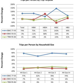
Total HBW HBSH HBSC HBO

BMC 77-93 74% 75% 31% 143% 44%

BMC 93-01 -3% -11% 68% -54% 8%

TRM 95-06 1% -19% 2% -23% 31%

-100% -50% 0% 50% 100% 150% 200% Per cen t C ha ng e

Trips per Person by Trip Purpose

BMC 77-93 77% 62% 78% 74%

BMC 93-01 -7% -1% -5% -6%

TRM 95-06 -1% 0% 5% 1%

-20% 0% 20% 40% 60% 80% 100% Per cen t C ha ng e

Trips per Person by Household Size

BMC 77-93 103% 74% 57% 36%

BMC 93-01 1% 0% -3% -9%

TRM 95-06 0% 0% 1% 3%

-20% 0% 20% 40% 60% 80% 100% 120% Per cen t C ha ng e

(59)

0 to 4 5 to 19 20 to 44 45 to 64 65 or _older

BMC 1980-1990 20% -21% 10% -8% 15% BMC 1990-2000 -14% 10% -12% 20% 4% TRM 1980-1990 12% -20% 9% -2% 5%

TRM 1990-2000 0% 6% -8% 20% -7%

-25% -20% -15% -10% -5% 0% 5% 10% 15% 20% 25% Per cen t C ha ng e

Population by Age

BMC 1990-2000 15% 0% -9% -10%

TRM 1980-1990 17% 4% -4% -17%

TRM 1990-2000 1% -1% -7% 6%

-20% -15% -10% -5% 0% 5% 10% 15% 20% Per cen t C ha ng e

Households by Household Size

BMC 1990-2000 -8% 8% -2% -3%

-20% -15% -10% -5% 0% 5% 10% Per cen t C ha ng e