Copyright1999 by the Genetics Society of America
The Genetic Analysis of Age-Dependent Traits:
Modeling the Character Process
Scott D. Pletcher*
,†and Charles J. Geyer
†*Department of Ecology, Evolution and Behavior and†School of Statistics, University of Minnesota, Saint Paul, Minnesota 55108
Manuscript received March 15, 1999 Accepted for publication June 22, 1999
ABSTRACT
The extension of classical quantitative genetics to deal with function-valued characters (also called infinite-dimensional characters) such as growth curves, mortality curves, and reaction norms, was begun by Kirkpatrick and co-workers. In this theory, the analogs of variance components for single traits are covariance functions for function-valued traits. In the approach presented here, we employ a variety of parametric models for covariance functions that have a number of desirable properties: the functions (1) are positive definite, (2) can be estimated using procedures like those currently used for single traits, (3) have a small number of parameters, and (4) allow simple hypotheses to be easily tested. The methods are illustrated using data from a large experiment that examined the effects of spontaneous mutations on age-specific mortality rates in Drosophila melanogaster. Our methods are shown to work better than a standard multivariate analysis, which assumes the character value at each age is a distinct character. Advantages over existing methods that model covariance functions as a series of orthogonal polynomials are discussed.
S
INCE the introduction of quantitative genetics the- function of some independent and continuous variable.ory and methods to the study of evolution, a tremen- More specifically, a function-valued trait is a function
dous body of literature has developed, documenting x(t). In all of the work that has been done on
function-patterns of quantitative genetic variation within and be- valued traits, including ours, both the independent
vari-tween species for a wide variety of continuous characters able t and the dependent variable x(t) are single valued.
(Barton and Turelli 1989; Falconer 1989; Lynch These traits have also been called infinite-dimensional andWalsh1998). Evolutionary biologists use this infor- traits (Kirkpatrick and Heckman 1989) because the
mation to predict how a population might respond to character can take on a value at an infinite number of
natural or artificial selection and to provide insight into ages. In principle, there is no reason why our methods
the contributions of the various evolutionary processes or those of other workers in this area cannot be
ex-to the levels of genetic variation seen in natural popula- tended to allow t or x(t) or both to be multivariate. For
tions (Lande1979, 1982;Houle1992). Empirical esti- the case of univariate t and x(t), we think “function
mates of genetic variances in single traits and genetic valued” is the more descriptive term. It avoids confusion
covariances between traits have contributed greatly to with characters that are described by a multidimensional
our knowledge of the evolution of biological characters. t or x(t). For specificity, we always refer to the
indepen-Classical quantitative genetics theory covers the analy- dent variable t as time or age, although there is no
sis of a single quantitative trait, such as bristle number reason why it cannot be any continuous variable.
in Drosophila, or at most a few traits. However, many In cases where the functional nature of the trait is
interesting characters are inherently too complex to be of interest, classical methods are often employed by
described by classical theory. Most often this is because treating arbitrary, discrete age intervals as unique
char-it is difficult to describe the character of interest by a acters in a multivariate analysis (Hughesand
Charles-single value. Examples can be found in the field of life worth1994;Promislowet al. 1996;Tataret al. 1996;
history evolution, where traits change over the lifetime Pletcher et al. 1998). This approach is problematic.
of an individual. In fact, in many cases it is the change As the number of ages of interest increases the ability
of the character with age that is the primary interest to produce precise estimates of statistical parameters
(HughesandCharlesworth1994;Promislowet al. is rapidly lost (
Shaw 1987, 1991). In addition, when
1996;Pletcheret al. 1998).
measurements are taken at irregular intervals, one Function-valued traits are characters that change as a
might reasonably expect the trait to be more similar between ages separated by a short time as compared with more disparate ages. A standard variance component
Corresponding author: Scott D. Pletcher, Max Planck Institute for
analysis ignores this type of information.
Demographic Research, Doberaner Str. 114, D-18057 Rostock, Germany.
E-mail: [email protected] Recognizing the limits of the classical approach,
patrick andHeckman (1989) formulated a quantita- Cov(eij, ekl)5 dikεjl, (2a)
tive genetic model for function-valued traits, which has
wheredikare the elements of the identity matrix (dik5
since served as the foundation for numerous theoretical
1 if i5k, anddik5 0 otherwise), and
and experimental investigations in this area. On the
theoretical side, age-specific selection on a character Cov(gij, gkl)5 rikgjl, (2b)
and its interactions with genetic constraints have
re-where the rij are the coefficients of relationship
(ele-ceived considerable attention (Kirkpatricket al. 1990;
ments of the A matrix) and thegjlandεjlare parameters
Kirkpatrick and Lofsvold 1992). The evolution of
to be estimated. Making matrices G and E with elements
reaction norms over continuous environments has also g
jl andεjlallows us to write the matrix equation
been studied (GomulkiewiczandKirkpatrick1992).
On the experimental side, estimates of genetic variation Var(x)5 A^G 1I^E, (3)
for age-dependent growth patterns in birds (
Gebhardt-where ^ denotes the Kronecker product of matrices
Henrich and Marks 1993; Bjorklund 1997), mice
(Searleet al. 1992, pp. 443 ff.) and x is a vector con-(Kirkpatricket al. 1990;MeyerandHill1997), and
taining all data on all individuals in the order x11, x12,
livestock (Kirkpatrick 1997) have been published.
. . . , x21, x22, . . . . The matrices G and E are symmetric Moreover, the recent interest in age-specific
compo-m3m matrices if there are m traits, and each has m(m1 nents of genetic variation for other life-history
charac-1)/2 independent parameters. Statistical inference
ters (Engstromet al. 1989;Houleet al. 1994;Hughes
about the G matrix and the constraints it imposes on and Charlesworth 1994; Promislow et al. 1996;
the dynamics of phenotypic evolution is the primary
Pletcheret al. 1998) suggests that interest in
function-interest in these analyses (Lande 1979, 1982).
valued traits is growing.
Function-valued traits add an additional level of com-A quantitative genetics theory for function-valued
plication. Now for individual i the trait is a function traits is a straightforward extension to standard
method-xi(t) of the continuous variable t. Equations 2a and 2b
ology. Classical quantitative genetics partitions an
ob-are replaced by servable trait as
Cov{ei(s), ek(t)}5 dikE(s, t) (4a)
x5 m 1g1e, (1)
Cov{gi(s), gk(t)}5rikG(s, t). (4b)
where m is the mean (fixed effect) and g and e are
The primary interest in analyses of function-valued traits the genetic and environmental components (random
is statistical inference about the “G function,” G(s, t), effects). Assuming no gene-environment interaction, g
also called the additive genetic covariance function. The “E and e are independent, hence
function,” E(s, t), also called the environmental covariance
Var(x)5Var(g)1 Var(e). function, is of lesser interest.
In practice, data are only observed at a finite set of
If xi, etc. denote the effects for individual i, the simplest times t1, . . . , t
m, rather than a continuum, so we have
assumptions are that ei and ej are uncorrelated if i≠ j only a finite set of data on each individual, which we
and that Cov(gi, gj) is proportional to the coefficient of can consider as a multivariate trait vector x
i(t1), . . . ,
relationship of i and j (Falconer 1989, pp. 111 ff., x
i(tm). Although in theory the trait has a continuous G
especially p. 156). Making a matrix A of the coefficients function, in practice the covariance structure is
de-of relationship (the so-called numerator relationship ma- scribed by a “G matrix.” The elements of the G matrix
trix) allows us to write the matrix equation are genetic covariances between the trait measured at
different ages. The key idea here is that the elements
Var(x)5 s2
gA1 s2eI,
of the G matrix do not consist of unique parameters
where I is the identity matrix and s2
g and s2e are two for all variances and covariances. Instead, all elements
parameters to be estimated, the genetic and environ- of this matrix are obtained from a single G function.
mental variances. Thus, the finite dimensional G matrix for the character
More complex genetic models partition the genetic process model has elements defined bygjl5G(tj, tl). A
effect into additive, dominance, and other effects similar argument applies for the “E matrix.” Given the
(LynchandWalsh1998). All the theory and examples new parameterization of the G and E matrices, Equation
in this article consider only additive models. Extension 3 again describes the variance of the observed
pheno-of our methods to include dominance and other effects type considered as a multivariate trait vector xi(tj).
is theoretically straightforward (though no doubt some Is that all there is to function-valued traits? It appears
practical difficulties will arise). as though we have simply redefined the problem.
Al-When more than one trait is modeled, we have covari- though in principle there is a G function G(s, t), in
ances among traits as well as among individuals (Shaw practice there is only a G matrix G(tj, tl). Is anything
1987, 1991). If xij, etc., now denote the effects for individ- new introduced by talking about function-valued traits?
ods run into intractable difficulties when there are many
o
Ni51
o
N
j51
bibjrX(ti, tj)$0. (7)
traits. Even five traits are trouble (Shaw et al. 1995;
ShawandGeyer1997). Function-valued traits are often
Most quantitative genetics theory is based on the as-observed at many times (or many values of t if t is not
sumption that the character of interest or some transfor-time), too many for classical multivariate quantitative
mation of it is normally distributed (LynchandWalsh
genetics to cope with.
1998). This assumption can be extended to a character Some new idea has to be added to manage the
param-process by utilizing the theory of Gaussian param-processes
eter explosion, m(m11) parameters to estimate in the
(Hoel et al. 1972; Kirkpatrick andHeckman 1989). genetic covariance matrix alone if data are observed at
A stochastic process X(t), t P T, is called a Gaussian
m times. In the theory of function-valued characters,
process if the vector (X(t1), X(t2), . . . , X(tm)) has a
the number of parameters in the finite dimensional G
multivariate normal distribution for every choice of matrix is equal to the number of parameters in the G
times t1, . . . , tm(Hoelet al. 1972). As with any Gaussian
function—this is independent of the number of ages
random variable, the distribution of a Gaussian process examined, and the task is to model and estimate the G
is completely determined by its mean and covariance function. There are two possible approaches:
paramet-function. ric and nonparametric. This article explores the use of
Using the language of Gaussian processes, we can parametric models for the G function. Kirkpatrick and
now complete our description of quantitative genetics co-workers and followers use an approach that is
non-for function-valued traits. We assume the observed phe-parametric in spirit, although for most experimental
notypic character process X(t) is a Gaussian process and designs it is missing some important features that one
can be decomposed analogous to (1) as expects in a nonparametric statistical method.
In the following sections we provide a brief review of X(t)5 m(t)1 g(t)1e(t), (8)
the seminal work in this area, while focusing on the
wherem(t) is a nonrandom function, the mean function
differences between previous work and our own. We
of X(t), and g(t) and e(t) are mean-zero Gaussian pro-present repro-presentative examples from an extensive
se-cesses that are independent of each other and have ries of simulations in which we compared our approach
covariance functions G(s, t) and E(s, t), respectively. with those suggested previously. We then illustrate the
By the independence of g(t) and e(t), the covariance various techniques using real data on mortality rates in
function of X(t) is given by P(s, t) as female Drosophila. Last, we summarize some of the
benefits of our character process model over previous
P(s, t)5G(s, t)1 E(s, t). (9)
methods and suggest promising avenues for future
theo-retical development. Each individual has a different realization of the
charac-ter processes X(t), g(t), and e(t). The covariance of the processes for different individuals we have already
de-GENERAL CONSIDERATIONS
rived as (4a) and (4b).
The probabilistic framework for modeling a function- Thus the character process approach, also called
func-valued trait is based on the theories of stochastic pro- tion-valued quantitative genetics, can be simply but
cesses. A stochastic process can be defined as a set of briefly described as replacing the Gaussian random
vari-random variables X(t), tPT, where T is a subset of the ables or random vectors of classical quantitative genetics
real line and termed the time parameter set (Hoelet by Gaussian stochastic processes and proceeding mutatis
al. 1972). A specific realization of a process (i.e., the mutandis. What we have described so far includes all
values of the random variables at each t) is called a sample approaches to function-valued quantitative genetics:
path of that process. We are interested in processes with that of Kirkpatrick and co-workers, that ofMeyerand finite variance, i.e., for which E{X(t)2},∞, the so-called
Hill(1997), and ours. The differences are in how the
second-order processes. In such cases, we can define a G and E functions are modeled and in how the models
mean function of the process by are fitted to data.
mX(t)5 E{X(t)}, tP T (5)
and a covariance function of the process by NONPARAMETRICS AND ORTHOGONAL
POLYNOMIALS
rX(s, t)5 Cov{X(s), X(t)}, s, tPT. (6)
In the approaches of Kirkpatrick and co-workers and Equation 5 is the function describing how the expected
of Meyer and Hill, the G and E functions are modeled value of the character changes with age, and (6)
de-by a linear combination of orthogonal Legendre polyno-scribes the covariance between the character at two
sepa-mials rate ages. The covariance function must be nonnegative
definite, that is, for any finite set of times (t1. . . tN) and
G(s, t)5
o
m
i50
o
m
j50
φi(s)φj(t)kij, (10)
where G is the covariance function, m determines the have a large number of parameters, most of which
number of polynomial terms used in the model, kijare have no simple interpretation. Specific
age-depen-unknown parameters to be estimated (the coefficients dent hypotheses are not easily tested.
of the linear combination), andφiis the ith Legendre
We avoid these problems by using parametric models
polynomial (Kirkpatrick and Heckman 1989;
Kirk-for the G and E functions. We discuss a large family
patricket al. 1990). A similar model is used for the E
of parametric models, each with a small number of function.
interpretable parameters, that satisfy theoretical re-Kirkpatrick and co-workers used fitting procedures
quirements and that as a group exhibit a wide variety that are no longer recommended, being superseded
of behaviors. We (likeMeyerandHill1997) use ML
by the methods ofMeyerandHill(1997), who used
to estimate parameters. C code, implementing these restricted maximum likelihood (REML). Meyer and Hill
procedures, is available from the first author.
estimated the parameters of the model (i.e., the kij in
Equation 10) for each model with a fixed set of Le-gendre polynomials, which corresponds to fixing m in
(10). They then used likelihood-ratio tests to determine PARAMETRIC CHARACTER PROCESS MODELS
a value of m that adequately fits the data.
Useful parametric models for covariance functions We have no argument with model fitting by maximum
are limited by several theoretical requirements. First, likelihood (ML) or REML, but we propose a different
covariance functions must be positive semidefinite, i.e., way of modeling G and E functions. Covariance
func-satisfy Equation 7. Second, biological processes are ex-tions modeled with Legendre polynomials (or other
pected to be reasonably smooth, requiring their covari-orthogonal polynomials) have a number of potential
ance functions to be smooth as well (Hoelet al. 1972).
drawbacks.
If a Gaussian stochastic process is to be considered
1. They are not automatically positive semidefinite. Al- smooth, it will have differentiable sample paths, and so
though constrained ML or REML can be used to must its covariance function. In general the covariance
impose this condition, this greatly complicates hy- function has twice as many derivatives as the process
pothesis testing and other statistical procedures. itself (Hoelet al. 1972). Thus, because we expect
biolog-2. Legendre polynomials have no theoretical justifica- ical processes to be relatively smooth, we choose
covari-tion other than being one among many sets of or- ance function models that are highly differentiable.
thogonal basis functions. Third, it is desirable for the covariance function to have
3. Polynomials do not fit covariance functions well. parameters with biologically meaningful interpretations
Polynomials of high degree are extremely “wiggly”
so that interesting hypotheses can be easily tested. and do not have asymptotes. Sensible covariance
With these considerations in mind, we first concen-functions are extremely smooth and typically
trate on a simple model of a character process that nevertheless may adequately represent many age-depen-G(s, t)→0, as|s2t| → ∞
dent traits. We assume each process X(t) is second-order
(an asymptote). stationary, which means
4. For the majority of genetic studies, trying to be
non-parametric about the covariance function of an un- mX(t) is independent of t and
observable stochastic process may be optimistic. In rX(s, t) is a function of s2 t
time-series analysis and spatial statistics, where the
(Hoelet al. 1972). This stationarity assumption is neces-stochastic process is observed directly, the most
suc-sary for several fundamental results, but it is relaxed cessful methods use parametric models [e.g.,
autore-later. Second-order stationarity requires that the mean gressive integrated moving average (ARIMA)
model-value of the trait must not change with age and that the ing of time series and variogram estimation in spatial
covariance between the value of the character at two statistics]. Experience in spatial statistics shows that
different ages depends only on the time distance be-the behavior of be-the covariance function at points
tween the age classes. closely related in time determines most of the
behav-For stationary models, the choice of a covariance func-ior of the process, and it is difficult to distinguish
tion is greatly simplified by Bochner’s theorem (Hoelet
different behaviors in the tails of the covariance
func-al. 1972), which asserts that a strictly positive covariance
tion (Cressie 1993, section 3.2.1). It is even more
function is necessarily proportional to the characteristic difficult if the stochastic process is unobserved like
function of some probability distribution. Thus, imme-the genetic and environmental processes in
quantita-diately we have a long menu of potential covariance tive genetics. For realistic experimental designs,
functions from which to choose, as any real-valued char-there is not enough information in the data for good
acteristic function of a probability distribution is al-nonparametric estimation.
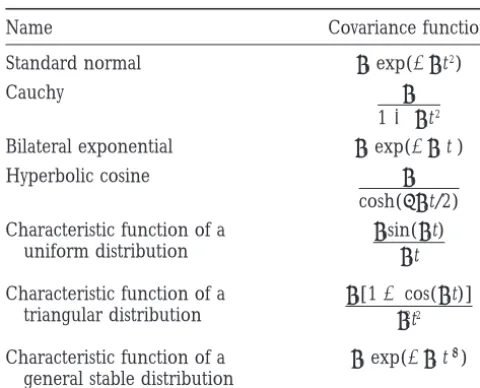
TABLE 1 (rather than covariance) stationarity. This relaxation
allows variance to change with age. IfrX(s2 t) is the
Covariance functions for the character process model
correlation function of a second-order stationary pro-cess and v(t) is an arbitrary function, then
Name Covariance function
rX(s, t) 5v(s)v(t)rX(s2t) (11)
Standard normal u0exp(2uct2)
Cauchy u0 is a valid covariance function. Thus we can chooserX(t)
11 uct2 to be any of the functions in Table 1 with the additional
restriction thatu0 5 1 [so that the correlation of X(t)
Bilateral exponential u0exp(2uc|t|)
with itself is 1] and choose v(t) completely arbitrarily
Hyperbolic cosine u0
cosh(puct/2) and still obtain a reasonable model. Although the model has stationary correlation, the variance
Characteristic function of a u0sin(uct)
uct
uniform distribution Var{X(t)}5v(t)2
is not stationary and can be specified as we please.
Characteristic function of a u0[12cos(uct)]
u2 ct2
triangular distribution Hypotheses concerning the pattern of change in age-specific variances (genetic and otherwise) for a given
Characteristic function of a u0exp(2uc|t|a) character can be examined using this model.
general stable distribution The parameters of the model are estimated
straight-forwardly using ML or REML. The reason, as mentioned
Valid covariance functions derived from the characteristic
functions of various probability distributions. The parameters in the Introduction, is that the character process is only
satisfyu0.0,uc.0, and 0, a #2. Characteristic functions observed at a finite set of times; hence the observations
were taken from Feller (1968). More general covariance
form a multivariate normal random vector with mean
functions can be obtained by replacingu0with a more general
and covariance that are specified by the models for the
variance function (see text).
mean function and G and E covariance functions. In principle the estimation procedure is no different from classical quantitative genetics of multivariate traits. Only in Table 1. In many cases the characteristic function
of one probability distribution is proportional to the the model specification is new. In practice, however,
the ideas of the character process model use reasonable probability density function of another. In such cases
we refer to the covariance function by the name of assumptions to reduce the dimension of the parameter
space and make an age-dependent quantitative analysis the distribution with the proportional density. In cases
where there is no such distribution, the covariance func- of the trait possible.
tion is specifically referred to as the characteristic func-tion of its parent distribufunc-tion. The available funcfunc-tions
EXAMPLES
exhibit a wide variety of behaviors, and some can be
negative in sign. Simulation study:We investigated the behavior of the
character process and orthogonal polynomial (OP) Although the assumptions of stationarity are rather
strict, we can use the results for stationary processes models through extensive simulations. Three
represen-tative examples are provided in this section. For each to formulate models that account for age-dependent
changes in the mean value of the character and that example, a single data set was generated assuming a
standard half-sib design (Lynch and Walsh 1998) in
allow for more general covariance functions. The
sim-plest way to achieve first-order stationarity (i.e., a con- which 20 sires were each mated to three dams and three
progeny were measured from each dam. We assumed stant mean over time) is to model the mean separately
as in (8), where g(t) and e(t) have mean zero for all the character of interest was measured at 10 regularly
spaced ages denoted 1, . . . , 10. It is important to note t, hence are first-order stationary. The nonstochastic
function m(t), analogous to fixed effects in classical that such a balanced design is not required for applying
these methods. Unequal family structure, as well as irreg-quantitative genetics, models the mean behavior. An
alternative to modeling the mean function directly is to ularly spaced measurements, are perfectly
accept-able, although different designs will contain different use methods analogous to those used to remove trends
in time series (Box et al. 1994), such as differencing amounts of genetic information (Shaw1987). Details
of the simulation procedure are available from the first the series (replacing the value at time t by Xt11 2Xt),
and more generally using “integrated” models, such as author.
Because they are unobserved, we have no way of know-ARIMA.
A relaxation of second-order stationarity—the condi- ing what a typical genetic covariance function might
look like. Therefore, these examples are rather arbitrary tion that requires the covariance of the process between
ages t1and t2to be only a function of|t12t2|—that still and serve mainly to illustrate the relationship between
Figure2.—(A) Actual genetic covariance surface for
simu-Figure1.—(A) Actual genetic covariance surface for
simu-lated data from case II: constant genetic variance and slowly lated data from case I: constant genetic variance and rapidly
declining covariance. The form of the covariance function is declining covariance. The form of the covariance function is
G(t1, t2)50.5e20.01(t12t2)2. (B) Lack of fit of an estimated genetic
G(t1, t2)50.5e20.7(t12t2)2. (B) Lack of fit of an estimated genetic
covariance surface for a model consisting of three orthogonal covariance surface for a model consisting of five orthogonal
polynomials. Lack of fit is defined as the absolute difference polynomials. Lack of fit is defined as the absolute difference
between the estimated surface and the actual surface. Darker between the estimated surface and the actual surface. Darker
regions indicate greater lack of fit. regions indicate greater lack of fit.
cally uncorrelated (or nearly so), OP models provide a relatively simple cases: case I, genetic variance is
con-poor estimate of the covariance function (Figure 1). stant across all ages, and genetic covariance declines
The five-polynomial model was determined to provide very quickly between adjacent ages; case II, genetic
vari-an adequate fit to the data via likelihood-ratio tests (a ance is constant across all ages, and genetic correlation
six-polynomial model did not fit significantly better), declines very slowly; case III, the genetic covariance
and although the fit is quite poor, genetic variances are function is composed of four OPs (giving a covariance
estimated more accurately than covariances (Figure 1b). function of degree three).
In our experience this is to be expected when covari-Figures 1–3 present the actual covariance functions
ances decline asymptotically toward zero within the for each of the three cases along with contour plots
range of the data. The wiggly nature of the polynomial describing the fit of different models to the simulated
model has difficulty reproducing such a structure. The data. The contour plots display the absolute difference
OP model does a much better job of describing the between the fitted surface and the actual surface, with
covariance structure when genetic correlations are high darker regions indicating regions of poor fit and lighter
between all ages in the data (Figure 2). In this case, the regions indicating regions of better fit. Contour shading
three-OP model was determined as the best fit, and is constant over all figures, allowing comparisons
be-it does a reasonable job of estimating the covariance tween them.
not presented for these two examples. They are ex- structure of the genetic covariances. Nevertheless, the fit of the character process model is not terrible, and pected to fit well (and do) because they were used to
generate the data. essentially smooths over the undulations in the actual
function. Surprisingly, the OP model has some difficulty Figure 3 presents a genetic covariance function
gener-ated directly from a four-OP model. In this case, it was reproducing the covariance structure. This is likely due
to the number of parameters in the model (10) and the character process model (a linear variance model
with normal correlation) that had trouble capturing the the size of the simulated experiment. Even when the
form of the underlying covariance function is known precisely, most experiments will not provide enough information to accurately estimate even a moderate number of parameters.
In summary, OP models do not accurately describe the structure of the genetic covariance function when the genetic correlation is expected to decline signifi-cantly with age. We argued (see above) that it is these types of covariance functions that one might expect from natural stochastic processes. For relatively simple covariance structures, however, the OP models accu-rately estimate the surfaces (Figure 2). Flexibility from the range of allowable character process models allows a reasonable approximation to the actual covariance structure even when it is very irregular (Figure 3). More-over, Figures 1–3 suggest that a significant strength of the character process model is its separation of variance functions from correlation functions. In all the exam-ples, the majority of lack of fit is in the covariance (not variance) structure, suggesting the overall fit of the model is determined primarily by estimates of age-spe-cific variances.
Age-specific mortality rates in Drosophila:In this ex-ample, our goal is to estimate the genetic covariance structure for age-specific mortality rates in lines of Dro-sophila melanogaster allowed to accumulate spontaneous
mutations for 19 generations (Pletcher et al. 1998).
The data are mortality rate estimates (5-day intervals) for 29 mutation-accumulation lines. For each accumulation line there are four mortality observations at each age, and mortality rates are presented for six different ages. A logarithmic transformation was used to normalize the
data (Promislowet al. 1996;Pletcheret al. 1998). In
this example, log-mortality rates are examined through age 30 days posteclosion. Data from the oldest ages were excluded because estimates of genetic variances and covariances among these ages were extremely imprecise when estimated using standard methods, and often this
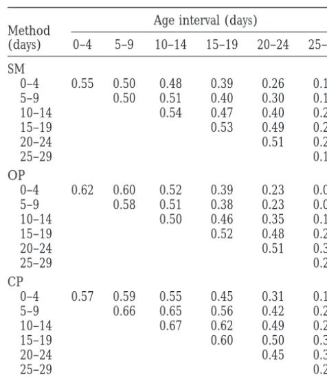
TABLE 2
hindered our ability to compare estimation methods.
Estimates of the mutational covariance structure based Comparison of age-specific genetic variance matrices
on the complete data set are presented in a companion estimated by various methods
article (Pletcheret al. 1999).
The data set was analyzed using three approaches. Age interval (days)
Method
First, the genetic covariance structure was estimated
(days) 0–4 5–9 10–14 15–19 20–24 25–29
completely nonparametrically (i.e., using standard
mul-SM
tivariate techniques) by specifying a separate parameter
0–4 0.55 0.50 0.48 0.39 0.26 0.11
for each age-specific variance and each covariance. Our
5–9 0.50 0.51 0.40 0.30 0.17
sample size was far too small to estimate all 21
parame-10–14 0.54 0.47 0.40 0.21
ters in the 636 covariance matrix simultaneously, and
15–19 0.53 0.49 0.26
we were forced to construct the matrix piecewise—by 20–24 0.51 0.29
examining ages two at a time. Pairwise covariances were 25–29 0.16
obtained using ML implemented in the program QUER- OP
CUS (Shaw 1987; Shaw and Shaw1992). Second, a 0–4 0.62 0.60 0.52 0.39 0.23 0.04
genetic covariance function composed of four Legendre 5–9 0.58 0.51 0.38 0.23 0.05
10–14 0.50 0.46 0.35 0.15
polynomials (giving a polynomial of degree three) was
15–19 0.52 0.48 0.26
estimated using ML procedures similar to those of
20–24 0.51 0.30
MeyerandHill(1997). Third, we used the character
25–29 0.20
process approach to estimate a genetic covariance
func-CP
tion based on a quadratic variance function and normal
0–4 0.57 0.59 0.55 0.45 0.31 0.17
correlation function (see Table 1).
5–9 0.66 0.65 0.56 0.42 0.24
The estimated genetic covariance matrices for the 10–14 0.67 0.62 0.49 0.29
various methods are presented in Table 2. Although all 15–19 0.60 0.50 0.32
procedures appear to capture the dominant aspects of 20–24 0.45 0.31
25–29 0.22
the covariance structure, several issues make the
charac-ter process approach desirable. First, using standard Genetic covariance (generated by spontaneous mutations)
multivariate methods, covariances and their asymptotic for age-specific mortality rates in female Drosophila melanogaster
standard errors were estimated pairwise and are too estimated by standard multivariate methods (SM), orthogonal
polynomials (OP), and the character process model (CP).
small when considering the matrix as a whole. Despite
The SM matrix was estimated “piecewise,” by estimating
vari-the small standard errors vari-there is insufficient statistical
ances and covariances between pairs of ages. The OP matrix
power to detect a significant change in covariance as
was based on a model of four orthogonal polynomials, and
ages become further separated in time (analysis not the CP matrix was based on a quadratic variance and normal
shown). Second, because data from each age are consid- correlation function.
ered separately, systematic relationships among the characters are ignored. Third, the sample size prohibits
estimating the entire 636 covariance matrix simultane- guaranteed to be positive definite, and data from all
ages are analyzed simultaneously. Standard errors for ously, and as a result the “piecewise” matrix (Table 2)
is not even positive definite. the parameters of the model are obtained from the
maximization procedure and error estimates on the in-The genetic matrix produced by the four-polynomial
model is quite similar to that produced by the standard dividual age measures can be easily calculated. Most
covariance functions have relatively few parameters, methods. However, a primary concern remains the
num-ber of parameters in the model; we are estimating 10 which are estimated with high precision. Finally, and
perhaps most importantly, the parameters of the model parameters for the genetic matrix alone. As with the
standard methods, the number of parameters demands have useful interpretations, which allow simple
hypothe-ses to be easily tested. a large sample size for accurate estimation, but unlike
these methods, none of the parameters have a clear To further investigate the behavior of the character
process models, we fit several different covariance func-interpretation. Although we may have asymptotic
vari-ance estimates for the coefficients of the OP (as is the tions to the data. In all models, we estimated a
nonpara-metric mean function—average mortality rates at each case when ML is used), it is difficult to establish simple
tests of interesting hypotheses. For example, the rate of age were estimated simultaneously—to account for the
increase in mortality rates with age. For both the genetic decline in covariance as ages become further separated
in time is described by a complicated combination of and environmental effects, we examined the fit of
covari-ance functions composed of (in all combinations) three the coefficients of the polynomial.
Many of the problems inherent in the standard and variance functions, the v(t)2 from Equation 11
(con-stant, linear, and quadratic) and three correlation func-OP methods are alleviated under the character process
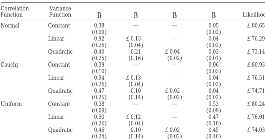
TABLE 3
Character process model estimates for genetic covariance functions
Correlation Variance
Function Function u0 u1 u2 uc Likelihood
Normal Constant 0.38 — — 0.05 280.65
(0.09) (0.02)
Linear 0.92 20.13 — 0.04 276.29
(0.26) (0.04) (0.02)
Quadratic 0.40 0.21 20.04 0.03 273.14
(0.25) (0.16) (0.02) (0.01)
Cauchy Constant 0.39 — — 0.06 280.93
(0.10) (0.03)
Linear 0.94 20.13 — 0.04 276.51
(0.26) (0.04) (0.02)
Quadratic 0.47 0.10 20.02 0.04 274.71
(0.25) (0.14) (0.02) (0.02)
Uniform Constant 0.38 — — 0.53 280.24
(0.09) (0.09)
Linear 0.90 20.12 — 0.47 276.01
(0.26) (0.04) (0.10)
Quadratic 0.46 0.10 20.02 0.45 274.03
(0.24) (0.14) (0.02) (0.10)
Parameter estimates (standard errors) and the log likelihoods for nine character process models composed of all combinations of three variance and three correlation functions. Variance functions are as follows: constant (u0), linear (u01 u1), and quadratic (u01 u1t1 u2t2). Correlation functions are taken from Table 1 withu051.
Estimates were obtained using maximum likelihood.
and characteristic function of a uniform). For all analy- is little statistical power to detect subtle differences in
the shapes of the underlying genetic correlation ses the constant variance and Cauchy correlation
func-tions were chosen for modeling the environmental co- tion.
Hypothesis tests concerning age-specific genetic vari-variance—more complicated covariance functions did
not provide a significantly better fit (details not shown). ance for mortality are easily conducted. ML estimates
are asymptotically normally distributed, and therefore Parameter estimates for the genetic covariance
func-tions are given in Table 3. The dynamics of age-specific their estimated standard errors can be used to construct
confidence intervals and test statistics (Searle et al.
genetic variance can be determined using
likelihood-ratio tests. Given a specific correlation function, twice 1992). Further, the significantly improved fit of the
qua-dratic variance function over the constant and linear the difference in log likelihoods between a more general
variance model (e.g., quadratic variance) and a more functions provides strong evidence for interesting
changes in mutational properties across ages, although constrained model (e.g., linear variance) has a
chi-square distribution with degrees of freedom equal to the the low variance at ages 25–29 days may be driving this
result. Such statements could not be made from the number of additional parameters in the more general
model. The P-values for the test that a quadratic variance results of standard methods or from the fit of OPs.
The hypothesis that most mutations affect mortality function fits better than a linear one are 0.01 for the
normal correlation function, 0.06 for the Cauchy, and equally at all ages can be tested by asking if the
correla-tion in mortality rates between various ages is different 0.05 for the characteristic function of the uniform (the
deviances being 6.3, 3.6, and 3.96, respectively, all from unity. Because, for all character process models,
uc(see Table 1) is the rate of decrease in correlation with asymptotically chi-square on 1 d.f.). A cubic variance
function did not provide a significantly better fit to the time, testing whether this value is significantly different
from zero directly addresses this hypothesis. The param-data.
Given a particular model for the variance function, eter is significantly greater than zero in all models (P,
0.05), providing strong evidence that the majority of there is little difference between the fits of the
correla-tion funccorrela-tions. For example, the log-likelihood values measured mutations exhibit some form of age
speci-ficity. for the normal, Cauchy, and uniform correlation
func-tions with a quadratic variance function are 273.14, Despite the twofold increase in the number of
param-eters, a covariance function based on four OP did not
274.71, and274.03, respectively. Although a rigorous
test of non-nested hypotheses such as these is rather provide a significantly better fit than the best-fit function
from the character process model. Using two popular
criteria, Akaike information criterion (AIC) and Bayes- Many of the problems with OPs were recognized by the original authors, and it has been suggested that
ian information criterion (BIC;Schwarz1978;Stone
1979), any of the character process models with a qua- more advanced “smoothing” techniques, such as
cubic-splines or wavelets, might be more well behaved (
Kirk-dratic variance function would be chosen over the best
OP model (data not shown). patrick et al. 1994). This is a promising avenue for
future research. Good parametric and nonparametric approaches complement one another. The strengths of
DISCUSSION
the parametric approach are its great efficiency and its ease of interpretation. Unfortunately, if the assumed The quantitative genetic analysis of function-valued
traits, such as growth and mortality curves, starts with model is grossly incorrect, inferences can be misleading
(Simonoff1996). Good nonparametrics are less reliant
the fundamental recognition by Kirkpatrick and
Heckman (1989) that the genetic and environmental on assumptions about the formal structure of the data. They do, however, require large sample sizes, much components of such traits should be modeled as
Gaussian stochastic processes. It continues with the rec- larger than many of the most ambitious quantitative
genetic studies. If there is insufficient information in
ognition byMeyerandHill(1997) that ML or REML
can be used to fit such models, just as it can be used the data to support the accurate estimation of many
parameters, one is essentially left with a bad parametric for all other quantitative genetics models. Our
contribu-tion to the subject is a method of finding valid paramet- model.
An equally promising direction for the future might ric models for covariance functions of these Gaussian
processes from theory in spatial and time-series statistics, be the extension of our techniques to examine the
rela-tionship between multiple character processes.
Two-where it is widely used (Cressie1993, section 2.5.1).
These parametric models for covariance functions character processes can be examined by estimating
co-variance functions for each character and a cross-have many virtues. They are assured to be positive
defi-nite, hence valid covariance functions. They can be cho- covariance function between the two (Kirkpatrick1988).
The approach is analogous to estimating the genetic sen to be highly differentiable, implying the character
process itself is smooth, which we expect from a biologi- covariance between two different characters, except in
this case the covariance is estimated for the value of the cal process. They have a small number of parameters,
and models can be chosen to address specific biological two characters at every combination of the two ages.
In this way age-dependent genetic constraints on the hypotheses. Moreover, the flexibility of the approach
means reasonable fits are obtained even when the actual independent evolution of the two traits can be explored.
covariance function is highly irregular (Figure 3). Comments provided by J. Curtsinger, R. Shaw, G. Oehlert, R. Lande,
It is important to recognize that parametric models M. Kirkpatrick, A. Clark, and an anonymous reviewer greatly improved
the quality and clarity of the manuscript. M. Kirkpatrick generously
have certain limitations. Although we have argued that
provided creative discussion throughout the development of this work.
our covariance functions are reasonable models,
veri-This work was supported by National Institutes of Health grants
AG-fying the assumptions of the models, particularly
sta-0871 and Ag-11722 to J. Curtsinger and by the University of Minnesota
tionarity in correlation, is exceedingly difficult (Math- Graduate School.
eron1988). Stationarity will, however, often be a good
approximation; and as George Box asserted, all models
are wrong, but some are useful (Box1976). Kirkpatrick LITERATURE CITED
and colleagues often focus on characterizing the
domi-Barton, N. H., andM. Turelli, 1989 Evolutionary quantitative
nant eigenfunctions of the genetic covariance function, genetics: how little do we know? Annu. Rev. Genet. 23: 337–370.
Bjorklund, M., 1997 Variation in growth in the blue tit (Parus
which are thought to summarize patterns of genetic
caeruleus). J. Evol. Biol. 10: 139–155.
variation (Kirkpatricket al. 1990). Although we have
Box, G. E. P., 1976 Science and statistics. J. Am. Stat. Assoc. 71:
not pursued it here, it is likely that for a particular covari- 791–802.
Box, G. E. P., G. JenkinsandG. C. Reinsel,1994 Time Series Analysis:
ance function, the eigenfunctions are somewhat limited
Forecasting and Control, Ed. 3. Prentice Hall, Englewood Cliffs, NJ.
in their range of behaviors. One may argue, however,
Cox, D. R.,1961 Tests of separate families of hypotheses. Proc. 4th
that the process of choosing a good model in effect Berkeley Symp. 1: 105–123.
Cox, D. R., 1962 Further results on tests of separate families of
searches a large space of possible eigenfunctions.
hypotheses. J. R. Stat. Soc. B 24: 406–424.
Implementing a nonparametric approach using
Le-Cressie, N. A.,1993 Statistics for Spatial Data. John Wiley and Sons,
gendre polynomials (KirkpatrickandHeckman1989) New York.
Engstrom, G., L. E. Lilijedahl, M. RasmusonandT. Bjorklund,
is problematic. Subsequent covariance functions are not
1989 Expression of genetic and environmental variation during
necessarily positive definite. Simple simulations show
ageing: 1. Estimation of variance components for number of
that polynomials of low degree do not closely approxi- adult offspring in Drosophila melanogaster. Theor. Appl. Genet. 77:
119–122.
mate reasonable covariance functions unless character
Falconer, D. S., 1989 Introduction to Quantitative Genetics, Ed. 3.
values at all measured ages are highly correlated
(Fig-Longman, New York.
ures 1 and 2). Polynomials of high degree have many Feller, W.,1968 An Introduction to Probability Theory and its
Applica-tions, Vol. 1, Ed. 3. John Wiley and Sons, New York.
Gebhardt-Henrich, S. G.,andH. L. Marks,1993 Heritabilities of Matheron, G.,1988 Estimating and Choosing: An Essay on Probability
growth curve parameters and age-specific expression of genetic in Practice. Springer-Verlag, New York.
variation under two different feeding regimes in Japanese quail Meyer, K.,andW. G. Hill,1997 Estimation of genetic and pheno-(Coturnix coturnix japonica). Genet. Res. 62: 42–55. typic covariance functions for longitudinal or ‘repeated’ records
Gomulkiewicz, R.,andM. Kirkpatrick,1992 Quantitative genetics by restricted maximum likelihood. Livest. Prod. Sci. 47: 185–200.
and the evolution of reaction norms. Evolution 46: 390–411. Pletcher, S. D., D. HouleandJ. W. Curtsinger,1998 Age-specific
Hoel, P. G., S. C. PortandC. Stone,1972 Introduction to Stochastic properties of spontaneous mutations affecting mortality in
Dro-Processes. Houghton Mifflin, Boston. sophila melanogaster. Genetics 148: 287–303.
Houle, D.,1992 Comparing evolvability and variability of quantita- Pletcher, S. D., D. HouleandJ. W. Curtsinger,1999 The
evolu-tive traits. Genetics 130: 195–204. tion of aspecific mortality rates in Drosophila melanogaster:
ge-Houle, D., K. A. Hughes, D. K. Hoffmaster, J. Ihara, S. Assima- netic divergence among unselected lines. Genetics 153: 813–823.
copouloset al., 1994 The effects of spontaneous mutation on Promislow, D. E. L., M. Tatar, A. A. KhazaeliandJ. W. Curtsinger,
quantitative traits. I. Variances and covariances of life history 1996 Age-specific patterns of genetic variation in Drosophila mela-traits. Genetics 138: 773–785. nogaster. I. Mortality. Genetics 143: 839–848.
Hughes, K. A.,andB. Charlesworth,1994 A genetic analysis of
Schwarz, G.,1978 Estimating the dimension of a model. Ann. Stat.
senescence in Drosophila. Nature 367: 64–66. 6:461–464.
Kirkpatrick, M.,1988 The evolution of size in size-structured
popu-Searle, S. R., G. Casella andC. E. McCulloch,1992 Variance
lations, pp. 13–28 in The Dynamics of Size-Structured Populations,
Components. Wiley and Sons, New York.
edited byB. EbenmanandL. Persson.Springer-Verlag,
Heidel-Shaw, F. H.,andC. J. Geyer,1997 Estimation and testing in
con-berg, Germany.
strained covariance component models. Biometrika 84: 95–102.
Kirkpatrick, M.,1997 Genetic improvement of livestock growth
Shaw, R. G.,1987 Maximum-likelihood approaches applied to
quan-using infinite-dimensional analysis. Anim. Biotech. 8: 55–56.
titative genetics of natural populations. Evolution 41: 812–826.
Kirkpatrick, M.,andN. Heckman, 1989 A quantitative genetic
Shaw, R. G.,1991 The comparison of quantitative genetic
parame-model for growth, shape, reaction norms, and other
infinite-ters between populations. Evolution 45: 143–151. dimensional characters. J. Math. Biol. 27: 429–450.
Shaw, R. G.,andF. H. Shaw,1992 QUERCUS: programs for
quanti-Kirkpatrick, M.,andD. Lofsvold,1992 Measuring selection and
tative genetic analysis using maximum likelihood. constraint in the evolution of growth. Evolution 46: 954–971.
Shaw, R. G., G. A. J. Platenkamp, F. H. ShawandR. H. Podolsky,
Kirkpatrick, M., D. LofsvoldandM. Bulmer,1990 Analysis of
1995 Quantitative genetics of response to competitors in Ne-the inheritance, selection and evolution of growth trajectories.
mophila menziesii: a field experiment. Genetics 139: 397–406.
Genetics 124: 979–993.
Simonoff, J. S.,1996 Smoothing Methods in Statistics. Springer-Verlag,
Kirkpatrick, M., W. G. HillandR. Thompson,1994 Estimating
the covariance structure of traits during growth and ageing, illus- New York.
trated with lactation in dairy cattle. Genet. Res. 64: 57–69. Stone, M.,1979 Comments on model selection criteria of Akaike
Lande, R.,1979 Quantitative genetic analysis of multivariable evolu- and Schwarz. J. R. Stat. Soc. Ser. B 41: 276–278.
tion, applied to brain:body size allometry. Evolution 33: 402–416. Tatar, M., D. E. L. Promislow, A. A. KhazaeliandJ. W. Curtsinger,
Lande, R.,1982 A quantitative genetic theory of life history evolu- 1996 Age-specific patterns of genetic variation in Drosophila
mela-tion. Ecology 63: 607–615. nogaster. II. Fecundity and its genetic correlation with mortality.
Lynch, M.,andB. Walsh,1998 Genetics and Analysis of Quantitative Genetics 143: 849–858.
Traits. Sinauer Associates, Sunderland, MA.