OPTIMIZATION APPROACH FOR SEWERAGE NETWORK DESIGN USING SEWER LINE DESIGN ALGORITHM

844 | P a g e

OPTIMIZATION APPROACH FOR SEWERAGE

NETWORK DESIGN USING SEWER LINE DESIGN

ALGORITHM

Daine, V. V.

, Dr.Rai, R. K.

Department of Civil Engineering, Government College of Engineering,

Amravati, Maharashtra, (India)

ABSTRACT

Wastewater collection systems encompasses components such as receiving drains, manholes, pumping stations that collects and transport the foul sewage from community to a sewage treatment plant or other place of disposal. A huge amount of investment is required for construction as well as maintenance of a wastewater collection systems, thereby substantially adding to the overall cost of the municipal sewerage system. Thus, reduction in cost of the collection system, at any point of the design, will provide significant savings towards the cost of municipal wastewater services. The design of sewerage network is governed by various constraints like branch depth, velocity, head loss, diameter, depth of flow etc.In the design of a sewerage network, a sewer line is a basic unit occurring repeatedly in the design-process and combining these basic units formulates the complete sewerage network. Cost of pipes, manholes and excavations adds to a major portion of the cost of sewer line. Thus, several studies, experiments and research works have been carried out to reduce the cost of a sewerage system through modified and improved optimum-seeking design methods. This paper pertains to the development of an optimization approach for the optimal design of a given sewerage network using sewer line design algorithm and dynamic programming.

Keywords: Dynamic programming, Optimization, Sewer, Sewer design, Sewer design algorithm,

Sewerage networks.

I. INTRODUCTION

Sewerage networks are integral part of the urban infrastructure and acquires a substantial position in the

sewerage system. A sewerage system consists of a network of sewer pipes laid throughout the area in order to

carry the sewage from individual houses, industrial and commercial areas to the sewage treatment plant or any

other point of disposal. Sewage collection, treatment and disposal systems are adopted to ensure that the sewage

discharged from communities is properly collected, transported and treated to the required degree in short,

medium and long-term planning and disposed-off without causing any health or environmental problems.The

investment needed for construction and maintenance of these large-scale networks is so huge that any saving in

the cost of these networks may result in considerable reduction in the total cost of a sewerage system. Thus,

845 | P a g e

is to develop a simple model for the optimal design of sewerage network using sewer line design algorithm with

Manning equation as the hydraulic model and dynamic programming as an optimization tool. The design

procedure is explained with an illustrative 6-link sewerage network.

II. HYDRAULIC EQUATIONS

The method comprises of designing the sewers as circular concrete sections with sewer running partially full.

Manning equation is used as a hydraulic model which is given by:

(1)

Where, V = Velocity of flow, m/s; N = Manning coefficient of roughness; R = Hydraulic radius, m; and S = Slope of sewer pipe. The value of manning coefficient for concrete sewers is taken as 0.013 to 0.015 [1]. The

formulae used for the design of sewer running partially full are as follows:

(2)

(3)

(4)

(5)

(6)

Where, = central angle; = relative depth; = area ratio; = hydraulic mean depth ratio; = velocity ratio;

= discharge ratio.

III. COST FUNCTIONS

The cost of a sewerage network includes cost of major components such as sewer pipe, excavation and manhole

for which the objective cost function has to be developed considering various cost parameters of these major

components.

3.1. Cost of sewer pipes

The capitalized cost of the sewer Cm can be expressed as[2]:

(7)

Where, km and m = Cost parameters of pipe; L = Length of pipe, m; and D = Diameter of sewer, m. The values of cost parameters for RCC pipe, class NP III, for various diameters was taken from Schedule of Rates, 2015[3],

and were found to be km=7590.4Rs. per m, and m = 1.376.

3.2. Cost of excavation

The total cost of excavation is the sum of the cost of earthwork and sheeting and shoring of sewer trenches.

846 | P a g e

Cer = capital earthwork cost; ce = unit earthwork cost at ground level, Rs./m3; cr = increase in unit earthwork cost per unit depth, Rs./m4; du and dd = invert depth at upstream and downstream nodes, respectively, m; and w = width of sewer trench, m. The width of trench is given by [1]:

w = 1.0 D ≤ 0.6 m (9a)

w = D + 0.4 D> 0.6 m (9b)

The cost of sheeting and shoring of sewer trenches depends upon the surface area of side walls of excavation

trenches. The capital cost of sheeting and shoring of a sewer trench Ces can be written as:

(10)

Where, cs = unit capital cost of sheeting and shoring at ground level, Rs./m2; and crs = increase in unit sheeting and shoring cost per unit depth, Rs./m3. Combining Equations (8) and (10), and rearranging the terms, the

total capital cost of excavation Ce is given by:

(11)

Where, ke = earthwork cost coefficient given by:

(12)

Costs of earthwork, and sheeting and shoring were taken from Schedule of Rates, 2015 [3]. The values of cost

parameters for excavation were found to be ce = 68.89, Rs./m 3

; cr = 12.235, Rs./m 4

; cs = 199.28 Rs./m 2

; and crs = 19.787 Rs./m3.

3.3. Cost of manhole

The cost of a manhole depends on the depth of manhole. The capitalized cost of the manhole Ch can be expressed as:

(13)

Where, kh and bh= Manhole cost coefficients; dh = Depth of manhole, m. Depth of a manhole is the depth of the out-going sewer at the manhole. The cost of manhole for various depths was taken from Schedule of Rates,

2015 [3]. The values of cost parameters were found to be kh = 14954 Rs./m; and bh = - 7952.1.

3.4. Total cost

The total cost CT of a sewer line can be obtained by adding the cost of major components of the line together, and is given by:

(14)

IV. DESIGN CONSTRAINTS

A sewerage network is designed to carry peak or design sewage flow at design relative depth. For this, it has to

847 | P a g e

4.1

Velocity constraints

In order to keep solid matter in suspension, a certain minimum velocity of flow is required, to prevent clogging

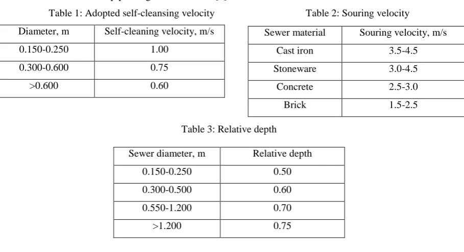
of the sewer; such a minimum velocity is known as self-cleansing velocity. The self-cleaning velocity varies

with the diameter of pipes as given in Table 1 [4].

At higher velocity, the flow becomes turbulent, resulting in continuous abrasion of the interior surface by the

suspended particles. To ensure that there is no damage or scouring of the pipe material, flow velocity is

restricted to a certain maximum limit. The maximum permissible velocity in the sewer line varies with the pipe

material as given in Table 2 [4].

4.2

Relative depth constraint

To maintain free surface flow, sewers are designed to flow partially full. The relative depth kd of the sewer pipe varies with the diameter of pipes as given in Table 3 [4].

Table 1: Adopted self-cleansing velocity Table 2: Souring velocity

Diameter, m Self-cleaning velocity, m/s

0.150-0.250 1.00

0.300-0.600 0.75

>0.600 0.60

Table 3: Relative depth

Sewer diameter, m Relative depth

0.150-0.250 0.50

0.300-0.500 0.60

0.550-1.200 0.70

>1.200 0.75

V. CONSTRAINT SATISFACTION

The basic goal is to minimize the cost of a sewer subjected to the relevant design criteria, hydraulic relationships

and design constraints. The usual constraints adopted in practice include minimum velocity, maximum velocity,

minimum cover, branch depth, relative depth and invert progression constraints. A sewer should have a

minimum cover depth hmin, which is generally taken to be between 1.0 m and 2.0 m [2]. The minimum depth at a node is D+hmin. The invert depth of the outgoing sewer should be greater than or equal to the invert depth of incoming sewers at the junction manhole.

VI. DESIGN ALGORITHM

The developed design algorithm for the optimal design of a sewerage network consist of the following steps:

1. Determination of set of feasible diameters for each link;

2. Determination of head loss and slope for each diameter;

Sewer material Souring velocity, m/s

Cast iron 3.5-4.5

Stoneware 3.0-4.5

Concrete 2.5-3.0

848 | P a g e

excavation and cost of manhole;

4. Design of all the links coming at junction manhole and selecting the links with minimum cost;

5. Extending the design with minimum cost and greater downstream invert depth up to next junction point and

design of all the links coming at that junction point;

6. Check the downstream invert depth of the extended design at previous junction with respect to other links at

that junction.

7. Repeat all the steps till outlet is reached.

The minimum and maximum feasible diameters can be obtained for a given flow using equations (1) to (6),

maximum and minimum velocities, and design relative depths. Assuming that the diameters are available at an

increment of 50 mm, the set of feasible diameters can be obtained for each sewer link. If the number of options

is insufficient, a few more options can be obtained by relaxing relative depth on lower side[5]. Relaxation

extents till the net decrease in head loss is 25 mm. Determine kvand kqfor each diameter using Equations (5) and (6), respectively. Determine flow and velocity at full flowing condition using flow and velocity at the partially

full flowing condition. Determine the slope for each option of a link and thereby head loss using the Manning

Equation.The upstream invert of first sewer depends on minimum soil cover and link diameter; its downstream

invert depends on the upstream invert, head loss and ground levels. Design all the sewer lines that meet at the

first junction point. Determine the cost of each line using Equations (7) to (14). Select the least cost options

from the designed lines at first junction point. Check the downstream invert depth of all the selected options and

further extend the design with greater downstream invert depth up to next junction point. Select the least cost

option from the extended design and check its downstream invert depth with respect to other selected options at

previous junction point. If the extended sewer line has greater downstream depth at previous junction point,

continue its design as main sewer line; else, redesign using the least cost option with greater downstream depth.

This process is continued till the extended sewer line option satisfies the downstream depth criteria at the

junction point. Further, select a maximum of 5 optimal solutions from the extended design and proceed using

the design process to the next junction[5].Similarly, determine the total cost of all the links coming at the next

junction point and select the least cost options from all the designed lines at that junction point. Check the

downstreaminvert depth of all the selected options and further extend the design with greater downstream invert

depth up to next junction point. The process is continued till outfall is reached and the optimal design of

sewerage network can be obtained by combining the least cost solution from all the steps.

VII. ILLUSTRATIVE DESIGN EXAMPLE

The design procedure for obtaining an optimal design of sewerage network is illustrated using a 5-link sewerage

network as shown in Fig. 1. The nomenclature adopted for the system consist three levels, where the first

number indicates the line number, the second indicates the pipe number, and the third indicates the option

number of feasible diameter for the pipe. The point where two or more links intersect is known as junction point

and the manhole at the point is termed as junction manhole. Two such junction manholes J1 and J2 are shown in Fig 1. The system outlet or sink for the sewerage network is located at the downstream end of pipe 1-3. The

849 | P a g e

VII. RESULTS AND DISCUSSION

The set of feasible diameters along with the corresponding head loss obtained for each linkof the sewerage

network is given in Table 5.

Table 5: Set of feasible diameters and head loss

Pipe Set of feasible diameters (head loss), m

1-1 0.550 (.185), 0.500 (.230), 0.450 (0.400), 0.400 (0.750), 0.350 (1.525), 0.300 (3.470)

1-2 0.800 (0.085), 0.750 (0.115), 0.700 (0.170), 0.650 (0.250), 0.600 (0.380), 0.550 (0.605),

0.500 (1.000), 0.450 (2.725)

1-3 1.000 (0.075), 0.950 (0.100), 0.900 (0.130), 0.850 (0.180), 0.800 (0.245), 0.750 (0.345),

0.700 (0.495), 0.650 (0.735), 0.600 (1.125), 0.550 (1.785)

2-1 0.300 (0.280), 0.250 (1.020), 0.200 (3.345)

2-2 0.400 (0.245), 0.350 (0.500), 0.300 (1.140), 0.250 (5.425)

3-1 0.550 (0.100), 0.500 (0.125), 0.450 (0.220), 0.400 (0.410), 0.350 (0.835), 0.300 (1.895)

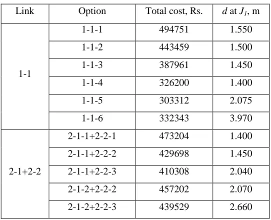
Considering the sewer pipe 1-1 as a starting point, slope and head loss for each diameter of link 1-1 were

determined; invert depths and total costs for each option were calculated. Similarly,the branch line 2-1 and 2-2

weredesigned together which produced 12 options and the invert depths and total cost for the best 5 out of 12

options were selected for further process. The cost and invert downstream depth at J1 is given in Table 6. Table 4: Design data for 6-link sewerage network

Pipe Q, m3/s Z1, m Z2, m L, m

1-1 0.10 158.0 157.2 110

1-2 0.25 157.2 156.5 120

1-3 0.45 156.5 155.8 110

2-1 0.03 158.0 157.6 75

2-2 0.06 157.6 157.2 100

3-1 0.10 157.0 156.5 60

850 | P a g e

Table 6: Cost and downstream invert depth oflinks at

J

Link Option Total cost, Rs. d at J1, m

1-1

1-1-1 494751 1.550

1-1-2 443459 1.500

1-1-3 387961 1.450

1-1-4 326200 1.400

1-1-5 303312 2.075

1-1-6 332343 3.970

2-1+2-2

2-1-1+2-2-1 473204 1.400

2-1-1+2-2-2 429698 1.450

2-1-1+2-2-3 410308 2.040

2-1-2+2-2-2 457202 2.070

2-1-2+2-2-3 439529 2.660

The least cost pipe options 5 and 2-1-1+2-2-3 were selected from line 1 and line 2 respectively. Option

1-1-5 has greater downstream invert depth than the option 2-1-1+2-2-3as shown in Table 6. Thus, sewer line 1 was

extended up to next junction point and designed with all the options of link 1-2 considering the upstream invert

depth of outgoing sewer pipe equal to or greater than the downstream invert depth of incoming sewer line at

junction J1, and the total cost of sewer line up to junction J2 was calculated. This process generated 48 options for the sewer line 1 up to the junction J2.The least cost solution for the sewer line 1 up to junction J2 is 1-1-4 + 1-2-7 have cost Rs.7.897 lakhsand downstream depth of1.400 mat J1.The downstream depth at J1 for the option 1-1-4 + 1-2-7 is less than the above selected sewer line option 2-1-1+2-2-3. Thus, the line 2 was extended and

designed as the main line with link 1-2 considering the upstream invert depth of outgoing sewer pipe equal to or

greater than the downstream invert depth of incoming sewer line at junction J1, and the total cost of sewer line up to junction J2 was calculated. This process generated 40 options for the sewer line 2 up to the junction J2. The variation in cost of the sewer line up to junction J2 is shown in Fig. 2. The optimal solution for the sewer line up to the junction J2 is 2-1-1 + 2-2-2 +1-2-7 having cost Rs. 9.017 lakhs (Fig. 2).

851 | P a g e

invert depth at junction point J1. The designed option 2-1-1 + 2-2-2 + 1-2-7have greater downstream depth at J1 and hence is selected as main line whereas the option 1-1-4 is separated and selected as the branch pipe.

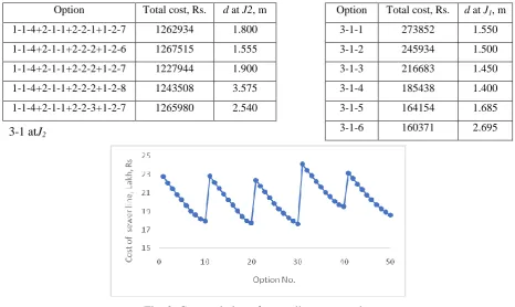
For further design process, five options with minimum cost is selected from the Fig. 2 and combined with the

cost of branch option 1-1-4. The total cost and invert downstream depth of the selected five options along with

the branch are shown in Table 7.

Similarly,slope and head loss for each diameter of line 3-1 coming at J2 were determined; invert depths and total costs for each option were calculated. The cost and invert downstream depth of option 3-1 is shown in Table 8.

From Table 8, option 3-1-6 having least cost was selected. The downstream invert depth of the sewer line 3-1-6

at J2 is greater than that of the designed option 1-1-4 + 2-1-1 + 2-2-2 + 1-2-7. Thus, sewer line 3 was extended further up to the outfall and designed with all the options of sewer link 1-3 by considering its upstream invert

depth equal to or greater than the invert depths of the sewer line 2 options coming at the junction J2. Total 60 options were obtained for the extended sewer line 3 along with sewer link 1-3.The least cost solution for the

sewer line 3 up to outfall is 3-1-4 + 1-3-10 having cost Rs.6.872 lakhs and downstream depth at J21.400 m. The downstream depth at J2 for the option 3-1-4 + 1-3-10 is less than the selected sewer line option 1-1-4 + 2-1-1 + 2-2-2 + 2-1-1-2-7. Thus, the line 2 was extended and designed as the main line with link 2-1-1-3 considering the

upstream invert depth of outgoing sewer pipe equal to or greater than the downstream invert depth of incoming

sewer line at junction J2, and the total cost of sewer line up to outfall was calculated. This process generated 40 options for the sewer line 2 up to outfall. The variation in cost of the sewer line up to junction J2 is shown in Fig. 3.

Table 7: Selected options of the sewer line up to

J

3-1 at

J

Fig. 3: Cost variation of sewer line up to outlet

Option Total cost, Rs. d at J2, m

1-1-4+2-1-1+2-2-1+1-2-7 1262934 1.800

1-1-4+2-1-1+2-2-2+1-2-6 1267515 1.555

1-1-4+2-1-1+2-2-2+1-2-7 1227944 1.900

1-1-4+2-1-1+2-2-2+1-2-8 1243508 3.575

1-1-4+2-1-1+2-2-3+1-2-7 1265980 2.540

Option Total cost, Rs. d at J1, m

3-1-1 273852 1.550

3-1-2 245934 1.500

3-1-3 216683 1.450

3-1-4 185438 1.400

3-1-5 164154 1.685

852 | P a g e

Rs.17.641 lakhs (Fig. 3). The optimal solution obtained from above was again checked for the downstream

invert depth at junction point J2. The designed option 1-1-4 + 2-1-1 + 2-2-2 + 1-2-7 + 1-3-10 have greater downstream depth at J2 and hence was selected as main line whereas the option 3-1-4 was separated and selected as the branch pipe. Thus, the cost of the option 1-1-4 + 2-1-1 + 2-2-2 + 1-2-7 + 1-3-10 was combined

with the cost of the selected link option 3-1-4 to obtain ultimate optimal solution. The total cost of the optimal

solution for the 6-link sewerage network comprising the pipe set 1-1-4 + 2-1-1 + 2-2-2 + 1-2-7 + 1-3-10 + 3-1-4

is Rs. 19.496 lakhs.

VIII. CONCLUSIONS

Following conclusions can be drawn from the present study:

1. The designed line algorithm was successfully applied to the given illustrative design example to obtain

optimal solution.

2. The optimal solution for a sewerage network can be easily obtained using the designed line algorithm.

3. The designed line algorithm can be used for the design of large sewerage networks.

4. The designed line algorithm does not involve numerous cost-effective grouping thus, reduces errors due to

large data handling.

5. The designed algorithm is an iterative process confined to depth constraints and the options become

cumbersome with increasing iterations at junction points.

REFERENCES

[1] Manual CPHEEO, Sewerage and sewage treatment, (Second Edition, Ministry of Urban Development,

1993).

[2] Swamee P. K., Design of sewer line, Journal ofEnvironmental Engineering, ASCE, 127(9), 2001, 776-781.

[3] Schedule of rates for Maharashtra Jeevan Pradhikaran works for the year 2015-2016, Amravati Region

(Amravati, 2015).

[4] Swamee P. K., Bhargava, R., and Sharma, A. K., Noncircular sewer design, Journal ofEnvironmental

Engineering, ASCE, 113(4), 1987, 824-833.

[5] Nagoshe, S. R., Rai, R. K., and Kadam, K. N., Optimization of sewerage network by dynamic