A study of reactive precipitation processes using computational fluid dynamics

(1)

A STUDY OF REACTIVE

PRECIPITATION PROCESSES USING

COMPUTATIONAL FLUID DYNAMICS

By

Mohsen Hassan Jaber AI-Rashed

B.Eng. (Hons) - Chemical Engineering (UCL) 1994

A Thesis Submitted to the

University of London

for the Degree of

Doctor of Philosophy

February 1998

Ramsay Memorial Laboratory

of Chemical Engineering

University College London

(2)

(3)

CFD & PRECIPITATION ABSTRACT

ABSTRACT

The objective of this research is to study and model a reactive precipitation process and determine the feasibility of applying the Computational Fluid Dynamics (CFD) technique. The CFX package of AEA Technology is adopted in this procedure. CFD is employed to model the batch gas-liquid reactive precipitation process of calcium carbonate in a 1.357 litre stirred vessel. Two major steps are involved in the modelling scheme, viz. the hydrodynamic model and the chemical kinetics and precipitation process model. Then, a link between these two models is created.

The hydrodynamic model considers the impeller as a momentum source. To predict the turbulence behaviour, the Reynolds differential stress model is implemented because it is more appropriate than the standard k-E model for swirling flows in stirred

tanks. The flow pattern is predicted for two-blade paddle impeller and details of the fluid speed, pressure and turbulent energy are produced. The same procedure is followed in modelling a 45° pitched-blade impeller with six blades, to show the effect of impeller type on the mixing process. Both 2-D and 3-D models are evaluated.

(4)

CFD & PRECIPITATION ABSTRACT

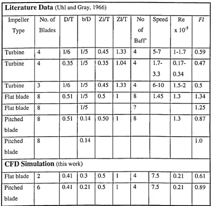
addition, flow number calculations from both the 2-D and 3-D CFD simulations show good agreement with literature data.

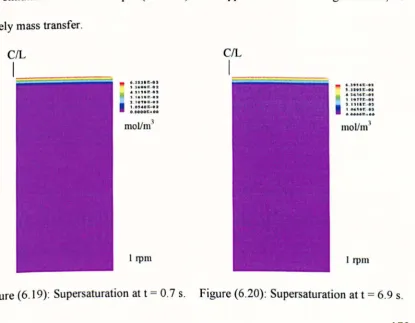
In order to minimise the computation time, the crystallization kinetics and precipitation process simulation is developed for a 2-D problem. The model calculates the extent of reaction, supersaturation, primary nucleation, size-independent crystal growth and the first four moments of the crystal size distribution throughout the vessel. Subsequently, the crystal average-mean size is evaluated. The model predicts an initial thin layer of particles forming in the interfacial region. The crystal slurry then starts to disperse into the bulk of the vessel following the flow pattern of the liquid. This behaviour is qualitatively comparable to the experimental results reported by Wachi and Jones (1991b).

The CFD model predictions are compared with those of the film and penetration theories for the same time range. The film theory shows a minor change in the mean size which indicates that it is a nucleation dominated process, i.e. high local supersaturation. Penetration theory predicts higher mean sizes, i.e. a growth dominated process with lower local supersaturation. The CFD simulation on the other hand, adopts an intermediate behaviour highlighting the role of the hydrodynamics in the process.

(5)

ACKNOWLEDGEMENTS

Praise and eulogy is for Allah for the blessing and bounties which He has bestowed. I would like to thank the following:

Professor Alan G. Jones for his supervision, support and encouragement throughout the project.

Timothy P. Elson for his precious discussion.

Crystallization group for their invaluable friendship and support. Technical staff for their assistance especially Martyn Vale. SPS and CFDS at the AEA Technology for funding this project.

Crystallization Panel of SPS for their constructive suggestions at the six-monthly progress meetings during the project.

The Overseas Research Students Award Scheme for the financial support. IUS founders, trustees, EC and members who made my university life distinctive, enjoyable and fruitful.

All My Friends.

(6)

"KNOWLEDGE ENABLES ITS POSSESSOR TO DISTINGUISH WHAT IS FORBIDDEN FROM WHAT IS NOT,' LIGHTS THE WAY TO HEAVEN,' IT IS OUR FRIEND IN THE DESERT, OUR COMPANION IN SOLITUDE, OUR COMPANION, WHEN BEREFT OF FRIENDS,' IT GUIDES US TO HAPPINESS,' IT SUSTAINS US IN MISERY,' IT IS OUR ORNAMENT IN THE COMPANY OF FRIENDS,' IT SERVES AS AN ARMOUR AGAINST

THE ENEMIES. WITH KNOWLEDGE THE

CREATURES OF ALLAH RISES TO THE

HEIGHTS OF GOODNESS AND TO NOBLE

POSITION, ASSOCIATES WITH THE

SOVEREIGNS IN THIS WORLD AND ATTAINS THE PERFECTION OF HAPPINESS IN THE NEXT. "

AL-MuSTAFA S.A. W.

(7)

"KNOWLEDGE ENABLES ITS POSSESSOR TO DISTINGUISH WHAT IS FORBIDDEN FROM WHAT IS NOT,' LIGHTS THE WAY TO HEAVEN,' IT IS OUR FRIEND IN THE DESERT, OUR COMPANION IN SOLITUDE, OUR COMPANION, WHEN BEREFT OF FRIENDS,' IT GUIDES US TO HAPPINESS,' IT SUSTAINS US IN MISERY,' IT IS OUR ORNAMENT IN THE COMPANY OF FRIENDS; IT SERVES AS AN ARMOUR AGAINST

THE ENEMIES. WITH KNOWLEDGE THE

CREATURES OF ALLAH RISES TO THE

HEIGHTS OF GOODNESS AND TO NOBLE

POSITION, ASSOCIATES WITH THE

SOVEREIGNS IN THIS WORLD AND ATTAINS THE PERFECTION OF HAPPINESS IN THE NEXT. "

AL-MuSTAFA S.A. W.

(8)

CFD & PRECIPITATION

Title Page

...

Dedication

...

Abstract

...

Acknowledgements

...

List of Figures

...

List of Tables

...

1. LITERATURE SURVEY

...

1.1. Crystallization

...

1.1.1. Supersaturation

1.1.2. Nucleation

...

1.1.3. Crystal Growth

1.1.4. Agglomeration

...

1.1.5. Aging

...

I.I.5a. Ripening

...

I.l.5b. Phase Transformation

1.1.6. Crystal Size Distribution (CSD)

1.1.7. Population Balances and CSDs

...

1.1.8. Precipitation Techniques

...

(9)

CFD & PRECIPITATION

I.I.8a. Precipitation by Direct Mixing

I.I.8b. Precipitation From Homogeneous Solution (PFHS)

I.1.8c. Salting-out

1.1.9. Determination of Crystallization Kinetics 1.1.10. Mass Balance Constraints

1.1.11. Moments of Crystal Size Distribution 1.1.12. Mass and Energy Balances

1.1.13. Driving Force for Mass Transfer 1.1.14. Residence Time Distribution (RTD) 1.2. Mixing Effects During Precipitation Processes

1.2.1. Introduction

1.2.2. Mass Transfer with Chemical Reaction and Precipitation

I.2.2a. Film Theory

I.2.2b. Surface Renewal Models I.2.2c. Empirical Models

1.3. Computational Fluid Dynamics

...

1.3.1. Introduction to Computational Fluid Dynamics

1.3.2. Fluids in Motion

1.3.3 Equations of Fluid Dynamics

1.3.3a. The Equation of Continuity 1.3.3b. The Equations of Motion

(10)

CFD Bc PRECIPITATION CONTENTS

1.3.4a. k-e model

1.3.4b. Reynolds Stress Model

92 93 1.3.5. Numerical Solutions to Partial Differential Equations 97

2.

1.3.6. Numerical Discretisation Techniques 1.3.6a. Finite Difference Method 1.3.6b. Finite Element Method 1.3.6c. Finite Volume Method

CFD, MIXING AND PRECIPITATION

.

... .

3. PRECIPITATION KINETICS AND SIMULATION

CONDITIONS

...

4. CFD HYDRODYNAMJC SIMULATION

Momentum Source -ImpeIler- Modelling

...

5. CHEMICAL KINETICS AND PRECIPITATION

PROCESS SIMULATION

...

6. RESULTS AND DISCUSSION

.

... .

6.1. 3-D Hydrodynamic Simulation

...

6.2. Hydrodynamic Simulation Validation

...

98 98 101 103

112

117

127

128

133

140

141 152 6.3. Chemical Kinetics and Precipitation Process Simulation 159

6.3.1. 1 rpm, Re = 4.6 Model

6.3.2. 100 rpm, Re = 4.6*103, Laminar Flow 6.3.3.100 rpm, Re = 4.6*103, Turbulent Flow 6.3.4.200 rpm, Re

=

9.3*103, Turbulent Flow 6.3.5.450 rpm, Re

=

2.1 * 104, Turbulent Flow

(11)

CFD & PRECIPITATION

7.

8.

9.

10.

11.

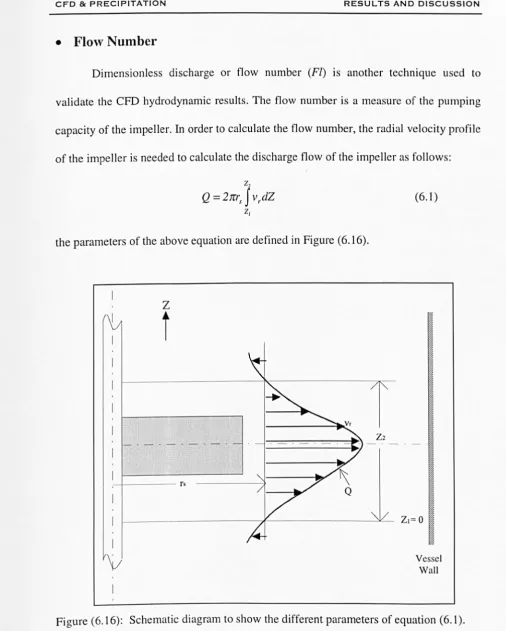
6.4 CFD Simulation Data analysis

...

6.5. Validation of the Chemical Kinetics and Precipitation

Process Simulation

CONCLUSIONS

.

... .

RECOMMENDATIONS AND FUTURE WORK

.

... .

NOMENCLATURE

LITERATURE CITED

.

... .

. ... .

APPENDIX

. ... .

CONTENTS

212

240

250

256

260

267

(12)

CFD & PRECIPITATION LIST OF FIGURES

LIST OF FIGURES

Figure (1.1): Solubility and primary nucleation in a hypothetical experiment. Figure (1.2): Schematic diagram of a simple, perfectly mixed crystallizer. Figure (1.3): Schematic diagram of a simple crystallizer.

Figure (1.4): Region of volume I1xl1yl1z fixed in space through which a fluid is flowing.

Figure (1.5): Volume element I1xl1yl1z with arrows indicating the direction in which

the x-component of momentum is transported through the surfaces. Figure (1.6): Location of points for Taylor series.

Figure (1.7): A two-noded linear element.

Figure (1.8): One-dimensional steady state diffusion problem.

Figure (1.9): Usual convention of CFD methods for one-dimensional problem. Figure (1.10): Two-dimensional grid convention.

Figure (1.11): A cell in three-dimensions and its neighbouring nodes.

Figure (3.1): Experimental apparatus.

Figure (3.2): (a) Two-blade paddle agitator and (b) six-blade 45° pitched impeller.

Figure (4.1): CFD Hydrodynamic simulation flow chart.

Figure (5.1): Chemical Kinetics and Precipitation process CFD simulation flow chart.

(13)

Figure (6.2): A view of the blocks from the CFD simulation.

Figure (6.3): The surface grid of the vessel.

Figure (6.4): The impeller region mesh at the centre of the vessel where the momentum source is defined.

Figure (6.5): Speed (m/s) vectors at the axial central plane (y=O).

Figure (6.6): Speed (m/s) shaded contours at the axial central plane (y=O).

Figure (6.7): Pressure (Pa)shaded contours at the radial central plane (z = 0.06 m). Figure (6.8): Pressure (Pa) shaded contours at the axial central plane (y

=

0).

Figure (6.9): Turbulent energy (m2/s2) shaded contours at the axial central plane (y=O).

Figure (6.10): Turbulent energy (m2/s2) shaded contours at the axial central plane (y=O).

Figure (6.11): Speed (m/s) shaded contours at the axial central plane (y = 0), for 45° pitched-blade impeller system.

Figure (6.12): Pressure (Pa) shaded contours at the axial central plane (y

=

0), for 45° pitched-blade impeller system.

Figure (6.13): Turbulent energy (m2/s2) shaded contours at the axial central plane (y

=

0), for 45° pitched-blade impeUer system.

Figure (6.14): A schematic diagram of the hydrodynamic experimental validation set-up.

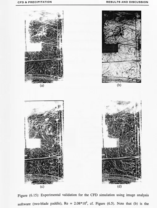
Figure (6.15): Experimental validation for the CFD simulation using image analysis software.

(14)

Figure (6.17): Radial velocity profile 2 mm away from the blade the two-blade paddle. Figure (6.18): Radial velocity profile 2 mm away from the impeller blade of the 45°

pitched blade.

Figure (6.19): Supersaturation at t = 0.7 s. Figure (6.20): Supersaturation at t = 6.9 s. Figure (6.21): Supersaturation at t = 14.4 s. Figure (6.22): Supersaturation at t = 30.3 s. Figure (6.23): Nucleation rate at t = 0.7 s. Figure (6.24): Nucleation rate at t = 6.9 s. Figure (6.25): Nucleation rate at t = 14.4 s. Figure (6.26): Nucleation rate at t = 30.3 s. Figure (6.27): Growth rate at t = 0.7 s. Figure (6.28): Growth rate at t = 6.9 s. Figure (6.29): Growth rate at t = 14.4 s. Figure (6.30): Growth rate at t = 30.3 s. Figure (6.31): Mo at t = 0.7 s.

(15)

Figure (6.40): M2 at t = 30.3 s.

Figure (6.41): Supersaturation at t = 2.0 s. Figure (6.42): Supersaturation at t = 12.4 s. Figure (6.43): Supersaturation at t = 17.8 s. Figure (6.44): Supersaturation at t = 30.1 s. Figure (6.45): Nucleation rate at t = 2.0 s. Figure (6.46): Nucleation rate at t = 12.4 s.

Figure (6.47): Nucleation rate at t = 17.8 s. Figure (6.48): Nucleation rate at t = 30.1 s. Figure (6.49): Growth rate at t = 2.0 s. Figure (6.50): Growth rate at t = 12.4 s. Figure (6.51): Growth rate at t = 17.8 s. Figure (6.52): Growth rate at t = 30.1 s. Figure (6.53): Mo at t = 2.0 s.

(16)

Figure (6.64): M2 at t = 30.1 s.

Figure (6.65): Speed vectors at the top-left and right corners of the vessel (lOO rpm, laminar).

Figure (6.66): Supersaturation at t

=

0.2 s. Figure (6.67): Supersaturation at t

=

5.1 s. Figure (6.72): Nucleation rate at t

=

1.3 s. Figure (6.74): Nucleation rate at t = 2.7 s. Figure (6.75): Nucleation rate at t

=

4.1 s. Figure (6.76): Nucleation rate at t = 4.5 s. Figure (6.77): Nucleation rate at t

=

5.1 s. Figure (6.78): Growth rate at t = 0.2 s. Figure (6.79): Growth rate at t = 1.3 s. Figure (6.80): Growth rate at t = 2.7 s. Figure (6.81): Growth rate at t = 4.1 s. Figure (6.82): Growth rate at t = 4.5 s. Figure (6.83): Growth rate at t = 5.1 s. Figure (6.84): Mo at t = 0.2 s.

(17)

CFD Bc PRECIPITATION LIST OF FIGURES

Figure (6.87): Mo at t

=

4.1 s. Figure (6.88): Mo at t

=

4.5 s. Figure (6.89): Mo at t

=

5.1 s. Figure (6.90): MI at t

=

0.2 s. Figure (6.91): MJ at t

=

2.7 s. Figure (6.93): M J at t

=

5.1 s. Figure (6.96): M2 at t

=

0.2 s. Figure (6.97): M2 at t

=

1.3 s. Figure (6.98): M2 at t

=

2.7 s. Figure (6.99): M2 at t

=

4.1 s. Figure (6.100): M2 at t

=

4.5 s. Figure (6.101): M2 at t

=

5.1 s. Figure (6.102): M3 at t

=

4.5 s. Figure (6.103): M3 at t

=

5.1 s.

(18)

CFD Bc PRECIPITATION LIST OF FIGURES

Figure (6.111): Supersaturation at t = 5.2 s.

Figure (6.112): CFD images of speed vector (m/s) superimposed on supersaturation (mol/m3) contours (Re = 9.3*10\ for t = 0.6, 1.3, 1.7 and 5.2 s for a, b, c and d, respectively.

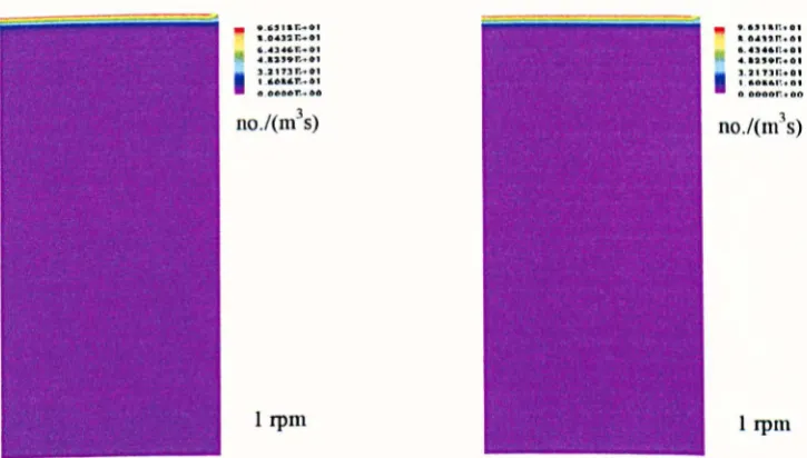
Figure (6.113): Nucleation rate at t = 0.2 s. Figure (6.114): Nucleation rate at t = 0.3 s. Figure (6.115): Nucleation rate at t = 0.6 s. Figure (6.116): Nucleation rate at t = 1.7 s. Figure (6.117): Nucleation rate at t = 3.5 s. Figure (6.118): Nucleation rate at t = 5.2 s. Figure (6.119): Growth rate at t = 0.2 s. Figure (6.120): Growth rate at t = 0.3 s. Figure (6.121): Growth rate at t = 0.6 s. Figure (6.122): Growth rate at t = 1.7 s. Figure (6.123): Growth rate at t = 3.5 s. Figure (6.124): Growth rate at t = 5.2 s. Figure (6.125): Mo at t = 0.2 s.

(19)

Figure (6.133): MI at t = 0.6 s. Figure (6.134): M I at t = 1.7 s. Figure (6.135): MI at t = 3.5 s. Figure (6.136): MI at t = 5.2 s. Figure (6.137): M2 at t = 0.2 s. Figure (6.138): M2 at t = 0.3 s. Figure (6.139): M2 at t = 0.6 s. Figure (6.140): M2 at t = 1.7 s. Figure (6.141): M2 at t = 3.5 s. Figure (6.142): M2 at t = 5.2 s. Figure (6.143): M3 at t = 3.5 s. Figure (6.144): M3 at t = 5.2 s.

(20)

Figure (6.157): Nucleation rate at t = 0.4 s. Figure (6.158): Nucleation rate at t = 0.6 s. Figure (6.159): Nucleation rate at t = 0.9 s. Figure (6.160): Nucleation rate at t = 1.3 s. Figure (6.161): Nucleation rate at t = 1.7 s. Figure (6.162): Nucleation rate at t

=

7.0 s. Figure (6.164): Nucleation rate at t= 10.0 s. Figure (6.165): Growth rate at t = 0.04 s. Figure (6.166): Growth rate at t

=

0.13 s. Figure (6.167): Growth rate at t

=

10.0 s. Figure (6.175): Mo at t

=

0.13 s.

(21)

(22)

Figure (6.205): M3 at t = 3.7 s. Figure (6.206): M3 at t

=

7.0 s. Figure (6.207): M3 at t

=

10.0 s.

Figure (6.208): Average supersaturation versus time for 1 rpm (Re

=

46) and 100 rpm (Re

=

4.6* 10\

Figure (6.209): A verage supersaturation versus time for 100 rpm (Re

=

4.6* 10\ 200 rpm (Re

=

9.3*103) and 450 rpm(Re

=

2.1 *104).

Figure (6.210): Mo versus time for 1 rpm (Re = 46) and 100 rpm (Re = 4.6*10\ Figure (6.211): Mo versus time for 100 rpm (Re

=

4.6*10\ 200 rpm (Re

=

9.3*103)

and 450 rpm (Re

=

2.1 * 104).

Figure (6.212): MI versus time for 1 rpm (Re = 46) and 100 rpm (Re = 4.6*103). Figure (6.213): MI versus time for 100 rpm (Re

=

4.6*10\ 200 rpm (Re

=

9.3*103)

and 450 rpm (Re

=

2.1 * 1 04).

Figure (6.214): M2 versus time for 1 rpm (Re

=

46) and 100 rpm (Re

=

4.6*10\ Figure (6.215): M2 versus time for 100 rpm (Re

=

4.6*103),200 rpm (Re

=

9.3*103)

and 450 rpm (Re

=

2.1 * 104).

Figure (6.216): M3 versus time for 1 rpm (Re

=

46) and 100 rpm (Re

=

4.6*10\ Figure (6.217): M3 versus time for 100 rpm (Re = 4.6*10\ 200 rpm (Re

=

9.3*103)

and 450 rpm (Re

=

2.1 * 1 04).

Figure (6.218): Average mean size versus time, for 1 rpm (Re = 46) and 100 rpm (Re

=

4.6*103).

(23)

Figure (6.220): Crystal mean size versus M3, for 1 rpm (Re = 46) after 30s and 100 rpm (Re = 4.6*103) after 10 s.

Figure (6.221): Crystal mean size versus M3 after 5 s, for 100 rpm (Re

=

4.6*10\ 200 rpm (Re = 9.3 * 103) and 450 rpm (Re

=

2.1 * 104).

Figure (6.222): The interface at the beginning of the process, (a) CFD model for Mo and (b) a picture of the experiment.

Figure (6.223): Particles start to disperse into the bulk from the interface region, (a) Mo from CFD model, (b) a picture of the experiment after 1 min.

Figure (6.224): More particles appear in the system following the flow pattern, (a) MO from CFD model, (b) a picture of the experiment after 3 mins.

Figure (6.225): CFD images of speed vector (m/s) superimposed on supersaturation (mol/m3) contours (Re

=

2.1 * 104), for t

=

0.04, 0.4, 0.6, 0.9 and 10.0 s for a, b, c, d and e, respectively.

Figure (6.226): Bulk supersaturation versus time from the penetration theory. Figure (6.227): Mo in the bulk versus time from the penetration theory. Figure (6.228): Crystal mean size versus time from penetration theory. Figure (6.229): Crystal mean size versus time from film theory.

Figure (6.230): Crystal mean size against time for CFD simulation, film and penetration theories.

Figure (A. 1 ): Figure (A.2):

Variation ofNp and Fl with Re, Sano and Usui (1987).

(24)

Figure (A3): Speed versus Distance for a line (x

=

-0.06 to 0.06, y

=

-0.06 to 0.06 and z = 0 to 0.12 m) in the vessel.

Figure (A.4): Vr versus axial distance at rs

=

0.027 m, for I rpm (Re

=

46).

Figure (AS): Vr versus axial distance at rs = 0.027 m, for 100 rpm (Re = 4.6* 10\ Laminar.

Figure (A6): Vr versus axial distance at rs

=

0.027 m, for 100 rpm (Re

=

4.6*10\ Turbulent.

Figure (A7): Vr versus axial distance at rs = 0.027 m, for 200 rpm (Re = 9.3* 1 03). Figure (A8): Vr versus axial distance at rs = 0.027 m, for 450 rpm (Re = 2.1 * 1 0\ Figure (A9): Speed vectors of the 2-D CFD simulations.

Figure (AI 0): 2-D model grid (48 x 24 cells) 0.12 x 0.06 m.

Figure (All): Film theory model computational flow chart, Wachi and Jones (1991 a). Figure (A12): Penetration theory model computational flow chart, Hostomsky and

(25)

CFD Bc PRECIPITATION LIST OF TABLES

LIST OF TABLES

Table (6.1): A comparison of Flow numbers from the literature and CFD simulation. Table (6.2): Average supersaturation versus time for 1 rpm (Re

=

46).

Table (6.3): Average supersaturation versus time for 100 rpm (Re

=

4.6* 103) with laminar flow.

Table (6.4): Average supersaturation versus time for 100 rpm (Re = 4.6* 103) with turbulent flow system.

Table (6.5): Table (6.6): Table (6.7):

Average supersaturation versus time for 200 rpm (Re

=

9.3*103) system. Average supersaturation versus time for 450 rpm (Re

=

2.1 * 1 04) system. Total Mo versus time, for 1 rpm (Re = 46).

Table (6.8): Total Mo versus time, for 100 rpm (Re = 4.6*103) with laminar flow. Table (6.9): Total Mo versus time, for 100 rpm (Re

=

4.6* 103) with turbulent flow. Table (6.10): Total Mo versus time, for 200 rpm (Re = 9.3* 10\

Table (6.11): Total Mo versus time, for 450 rpm (Re

=

2.1 * 104). Table (6.12): Total MJ versus time, for 1 rpm (Re

=

46).

Table (6.13): Total MJ versus time, for 100 rpm (Re

=

4.6*103) with laminar flow. Table (6.14): Total MI versus time, for 100 rpm (Re

=

4.6*103) with turbulent flow. Table (6.15): Total MI versus time, for 200 rpm (Re

=

9.3*103).

Table (6.16): Total MI versus time, for 450 rpm (Re = 2.1 *104). Table (6.17): Total M2 versus time, for 1 rpm (Re

=

46).

(26)

CFD Bc PRECIPITATION LIST OF TABLES

Table (6.21): Total M2 versus time, for 450 rpm (Re

=

2.1 * 104). Table (6.22): Total M3 versus time, for I rpm (Re

=

46).

Table (6.23): Total M3 versus time, for 100 rpm (Re = 4.6*103) with laminar flow. Table (6.24): Total M3 versus time, for lOO rpm (Re

=

4.6* 103) with turbulent flow. Table (6.25): Total M3 versus time, for 200 rpm (Re = 9.3*10\

Table (6.26): Total M3 versus time, for 450 rpm (Re

=

2.1 * 104).

Table (6.27): Average mean size calculated from Mo and M., for I rpm (Re

=

46). Table (6.28): Average mean size calculated from Mo and M .. for 100 rpm (Re

=

4.6*10\ laminar flow.

Table (6.29): Average mean size calculated from Mo and M .. for 100 rpm (Re

=

4.6*10\ turbulent flow.

Table (6.30): Average mean size calculated from Mo and M .. for 200 rpm (Re = 9.3*103).

Table (6.31): Average mean size calculated from Mo and M., for 450 rpm (Re = 2.1*10\

Table (A. I): The values of the parameters used in the simulation.

Table (A.2): Precipitation kinetics; set A is used in the CFD simulation, film and penetration theories (- 5 s.) and set B is used only for penetration theory (25 mins), Hostomsky and Jones (1995).

Table (A.3): The flow number values for the 2-D simulations. Table (AA): C02 concentration (kmol/m3).

(27)

(28)

CFD & PRECIPITATION LITERATURE SURVEY

1. LITERATURE SURVEY

1.1 Crystallization

The formation of a crystal can be characterised by two steps; the birth of a new

particle and its growth to macroscopic scale. The first step is known as nucleation. The

interaction of the rates of nucleation and crystal growth and the overall process

determines the crystal size distribution (CSD) in a crystallizer. The driving force for

both rates is supersaturation, and neither of the two steps can be achieved in a saturated

or under saturated solution, McCabe and Smith (1976). Thus, the first step to consider is

supersaturation.

1.1.1. Supersaturation

Supersaturation is defined rigorously as the deviation from thermodynamic

equilibrium, which is the difference between the chemical potential of the solute at the

existing conditions of the system J.1 and the chemical potential of the solute equilibrated

at the system conditions J.1 *, Rousseau (1993).

Four methods may produce a supersaturation, viz., cooling, evaporation,

salting-out and reaction. If the solubility increases significantly with temperature, then cooling

(29)

temperature. The salting-out method is applied when the other two processes are not

desired. In the third method a third component is added forming a homogeneous mixture

with the solvent in which the solute solubility is sharply reduced. However, if a

precipitation is required, the new solute may be created chemically by adding a third

component that will react with the original solute and form an insoluble substance,

McCabe and Smith (1976) and Sohnel and Mullin (1982).

Supersaturation can be expressed, with greater or lesser accuracy, in any of the

following formulations:

1. The difference between the chemical potential of the system and the chemical

potential at saturation, J.1-J.1 *, where J.1

=

J.1(T, c).

2. The difference between solute concentration and the concentration at equilibrium, c-c*.

3. The difference between the temperature at equilibrium and the actual temperature,

T*-T.

.

c

4. The relative saturatIOn, - .

c*

. . (c-c*)

5. The relative supersaturatIOn, S =

* .

c

The first formulation is the most fundamental, the second is particularly useful in

calculating the yield of a crystallizer, the third is usually employed in the control of a

crystallizer, and the fifth is often used in relating the dependence of nucleation and

(30)

1.1.2. Nucleation

The molecular rearrangement which leads to the development of a new ordered solid phase from a liquid or amorphous phase, and the thermodynamic and kinetic principles that initiate such arrangement, is called crystal nucleation (Zettlemoyer, 1969).

Nucleation mechanisms are classified into two types; homogenous and heterogeneous. In the former collisions on the molecular scale generate nuclei and in the later solid surfaces catalyse the nucleation process, Mersmann and Kind (1988).

(31)

CFD Se PRECIPITATION

M etastable lim it Cm - - --- --- - - --- -- -- - - - -- - -.C

c:: o

c::

Cl)

u c::

o

U

C*

-M etas tab le region

Solubility

rm

T*

Tern perature

LITERATURE SURVEY

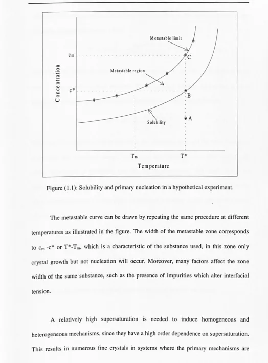
Figure (1.1): Solubility and primary nucleation in a hypothetical experiment.

The metastable curve can be drawn by repeating the same procedure at different

temperatures as illustrated in the figure. The width of the metastable zone corresponds

to cm -C* or T*-T rn, which is a characteristic of the substance used, in this zone only

crystal growth but not nucleation will occur. Moreover, many factors affect the zone

width of the same substance, such as the presence of impurities which alter interfacial

tension.

A relatively high supersaturation is needed to induce homogeneous and

heterogeneous mechanisms, since they have a high order dependence on supersaturation.

(32)

effective. The primary nucleation is dealt with according to the classical theory by the following equation (Rousseau, 1993):

(1.1)

where K is the Boltzman constant,

a

is surface energy per unit area, v is molar volume and A is a pre-exponential constant. By considering In(5+ 1) approaches s as s approaches zero, i.e. low supersaturation, equation (1.1) can be simplified as:

(1.2)

Equation (1.2) shows the factors that affect the nucleation rate, and the most important parameters are: interfacial energy, temperature and supersaturation. Due to the high order dependence of nucleation rate (Bo) on supersaturation, any small change in supersaturation may cause the nucleation rate to change dramatically. This explains the phenomenon observed of a clear liquor transformed to a slurry of fine crystals as a result of a slight change in supersaturation, e.g. by temperature drop.

In heterogeneous systems, the catalytic effect of solid particles is employed to reduce the energy barrier to formation of a new phase, i.e. reduce the interfacial energy

(a) significantly. The metastable limit can be obtained through experimentation, and

may be used to provide an empirical approach to model primary nucleation.

Empirically the nucleation rate is given as:

BO=k(c-c*)" _(1.3)

(33)

CFD Bc PRECIPITATION LITERATURE SURVEY

There is another type of nucleation called secondary nucleation. This is a crystal formation through mechanisms involving the solute crystal. Thus, in order to have secondary nucleation, solute crystals must already be present.

Secondary nucleation has special features which make it more important than primary nucleation in many industrial crystallizers. Primary nucleation, however, is thought to be the dominant mechanism during precipitation processes. The secondary nucleation features include: first, continuous and seeded batch crystallizers have crystals in the magma that can participate in the secondary nucleation mechanism. Second, employing the requirements for secondary nucleation is applicable in most industrial crystallizers. Finally, it is more favourable for most industrial crystallizers than primary nucleation, because those industrial crystallizers are operated at a low supersaturation which support secondary nucleation but not primary nucleation. A low supersaturation regime improves yield and enhances product purity and crystal morphology.

Secondary nucleation can be obtained following one of the identified mechanisms in selected systems.

1. Initial breeding: this mechanism IS important especially in seeded batch crystallization. It results from immersion of seed crystals in a supersaturated solution. It is also proposed that it is a result of dislodging extremely small crystals that were formed on the surface of larger crystals during drying.

(34)

required energy for contact nucleation is small and does not result in macroscopic degradation (breakage) of the contacted crystals.

3. Shear breeding: when a supersaturated solution flows by a crystal surface and carries with it crystal precursors believed formed in the region of growing crystal surface.

Many studies have investigated factors affecting contact nucleation. The number of crystals generated by a controlled impact of a particle with a seed crystal depends on energy of impact, supersaturation at impact, supersaturation at which crystals developed, hardness of the impacting particle, area of impact, angle of impact, and system temperature. It is impossible to quantify all of these variables, but some generalisations can be set from studying such nucleation mechanism.

For constant supersaturation systems, the following equation was proposed on experimental basis, Rousseau et al. (1976):

BO

= kNexp(E - Et) (lA)

It was also suggested that a relation of impact energy, E, to crystaIIizer variables must include the mass of the impacting crystal II1c , the rotational velocity of the impeller providing mixing

ro,

and the fraction of the available energy actually transmitted to the

crystal E:

(1.5)

(35)

CFD Sf PRECIPITATION LITERATURE SURVEY

resistance to diffusion or convective mass transfer. Furthermore, supersaturation affects the solution structure and causes the formation of clusters of solute molecules. These clusters may participate in nucleation, but again the mechanism of this is not clear. The contact nucleation mechanism dominates in many industrial operations, because of the ease with which nuclei can be produced by this mechanism, Rousseau (1993).

1.1.3. Crystal Growth

Growth kinetics are governed by at least two types of resistance. The first, resistance related to integration or incorporation of the crystalline unit into the crystal surface. The second, molecular or bulk transport of the unit from the surrounding solution to the crystal face, Small wood (1977) and Nancollas and Reddy (1971). The former is of a prime concern here.

Various growth models have been suggested to describe surface reaction kinetics, including models that assume crystals grow by layers and others that propose growth to occur by the movement of a continuous step. Thus, each model gives a particular relationship between growth rate and supersaturation, but none is applicable for a priori predictions of growth kinetics.

(36)

two-CFD Bc PRECIPITATION LITERATURE SURVEY

dimensional nucleation (MTDN) theory and the polynuclear two-dimensional nucleation (PTDN) theory are generated from the relative rates at which those two steps occur. The MTDN theory assumes that the surface nucleation step occurs at a finite rate, but the spreading across the surface is assumed to occur at an infinite rate. Whereas for the PTDN theory, the reverse is true. The MTDN theory relates growth to supersaturation as follows:

G = Cl hA.J1n(1 + s)ex

p[-

2 C2 ]

T

1n(1 + s) (1.6)

where the parameters Cl and Cz are system-dependent constants, h is the height of

nucleus, A is the surface area, s is the relative supersaturation and T is the system temperature. The PTDN theory results in the following relationship:

G - 3 ex _ 2

(

C ) [ C ]

- T2[ln(1

+

S)]3/2 p T21n(1

+

s) 0.7)

where C₃ is a system-dependent constant. Finally, if both formation of the two-dimensional nucleus and spreading of the surface layer are important in predicting the growth rate, the following derivation can be obtained:

(1.8)

where C4 is a system-dependent constant.

Since the quantity s is much less than 1, equations (1.6) to (1.8) can be simplified. The term, In(l +5), may be approximated to s. Consequently, the MTDN theory becomes:

(37)

For the PTDN theory:

(1.10)

and for both steps occurring at similar rates:

(1.11)

The screw dislocation or BCF theory (Burton, Cabrera and Frank, 1951), shows that the relationship between growth and supersaturation changes from a parabolic to linear as the supersaturation varies from low to high values, respectively. The growth rate is given by the BCF theory as:

(

es

2 )

[(j' ]

G = C

(j;

tanh

e~

( 1.12)

where E is screw dislocation activity and

<1;

is a system-dependent quantity that is

<1;

cc: (1 / T). An empirical approach is also obtainable to relate growth kinetics to

supersaturation with a power-law function of the form:

(1.13)

where kG and g are constants determined by fitting the equation to growth-rate data. However, such type of approaches is valid for a small ranges of supersaturation.

In the models described above, the temperature of the system has a pronounced effect on the growth rate. The relation between growth kinetics and temperature is often given by Arrhenius expression, Mersmann (1995):

(38)

where ko is a growth rate coefficient of the type required in equation (1.13), k~ is a

constant and Eo is an activation energy. Different effects are expected from both supersaturation and temperature. These effects influence the growth rates of different faces of the same crystal.

Impurities usually cause a reduction in the growth rates of crystalline materials, therefore obtaining smaller crystals than required is a common problem which is related to contamination of the feed solution. Certain operating conditions must be employed to minimise the possibility of such problems. Monitoring the composition of recycle streams can be advantageous in predicting the possible accumulation of impurities.

Two sets of factors are often attributed due to the outcome of a solvent in growth rates. One deals with the effects of solvent on mass transfer of the solute through adjustments in viscosity, density and diffusivity. The second considers the structure of the interface between crystal and solvent. It is concluded that a solute-solvent system with a higher solubility is likely to produce a rough interface and concomitantly large

crystal growth rates.

(39)

The rate of change of a crystal mass dM/dt is related to the rate of change in

crystal characteristic dimension by the equation:

( 1.15)

where pc is the crystal density and kv is the volume shape factor. Since an area shape

factor, ka may be defined by the equation:

( 1.16)

and G is defined as dLldt, therefore:

dMc

=

₃

(~)A

_G

dt Pc k C a

( 1.17)

The definition of growth rate, as the rate of change of the characteristic dimension, is

needed for the formulation of a population balance:

G= dL

dt ( 1.18)

and the resulting differential population balance has a solution which requires a

knowledge of the relationship between growth rate and size of the growing crystals. In

the mean time, this relationship can often be derived from the form of population

density data. One of the special cases is that when all crystals in the magma have the

same growth rate. If the crystals of the same size have different growth rates in the same

environment, they are said to exhibit anomalous growth.

Anomalous growth means that growth rates of crystals in a magma are not the

same or that the mass of crystals is not constant. There are two theories explaining

(40)

affect the form of the population density function that results from perfectly mixed continuous crystallizers, but this behaviour is inefficient to differentiate between the two theories, since they have the same qualitative effects on population density.

Correlating the apparent effect of crystal size on growth rate is attempted by many empirical expressions. The most commonly used correlation is:

(1.19)

Three parameters are involved in it; GO, y and b and they are determined from

experimental data. Although several theories have been suggested to explain the size-dependent growth kinetics, none has been substantiated by direct observation or used to determine the onset of such behaviour. One explanation shows some applicability, that is: large crystals have higher frequency and energy than smaller crystals during the impact with impeIIers and other crystaIIizer internals. Thus, the larger crystals are recipients of more surface breaks and irregularities that lead to higher growth rates. This theory proposes different crystal growth rates in a magma, although they may have identical sizes and the same conditions are employed.

There is experimental support for two different mechanisms describing growth dispersion. One assumes that all crystals have identical time-averaged growth rate, while individual crystals have fluctuating growth rates about some mean value. The other suggests that the formation of crystals is linked with a characteristic distribution of growth rates, but individual crystals retain a constant rate throughout their residence in a

(41)

The major factor in both mechanisms of growth rate dispersion is surface

integration. The number, sign and location of screw dislocations on the surface of a

growing crystal influence the growth rate, this is illustrated by the BCF theory. Changes

in the dislocation network occur as a result of a number of reasons: (1) collision of

crystals with each other and crystallizer internals and (2) imperfect growth of crystal

faces. The first leads to random fluctuations of growth rates. The varying dislocation

networks and densities among nuclei and seed crystals, produce the distribution of

growth rates.

Two different mechanisms are proposed for incorporating both mechanisms of

growth rate dispersion into descriptions of crystal population: the first is a random

growth rate and the second is the growth rate distributions. In order to clarify the relative

influences of the two mechanisms on CSDs from batch and continuous crystallizcrs,

both mechanisms can be included in a population balance.

1.4. Agglomeration

As mentioned earlier, agglomeration occurs just after nucleation, where small

particles in liquid suspension have a tendency to cluster together. If the particles are

small enough for the van der Waal forces to exceed the gravitational forces, then the

interparticle collision may result in a stable new larger particle. The above constraint is

(42)

The required time to halve the number of particles in monodisperse system is

called the half-time t*, which is given by the expression, Smoluchowski (1918):

(1.20)

where nt and no are the numbers of particles at t = t and t = 0, respectively. If an arbitrary

agglomerated system is defined as one in which more than 10% of particles have

agglomerated in less than 1000 s, then aqueous systems containing less than 107 cm·3• However, agglomeration is quite common in systems that have nucleated

homogeneously when n often exceeds 107 cm-3• In general, not all interparticle collisions result in permanent contact, and charge stabilisation in lyophopic systems has

a major influence in decreasing the rate of agglomeration.

Two types of agglomeration are reported for colloidal particles in suspension,

Smoluchowski (1918):

1. Perikinetic (static fluid, particles in Brownian motion)

2. Orthokinetic (agitated dispersion, fluid shear)

Precipitation processes involve both modes, but orthokinetic agglomeration

dominates in a stirred precipitator. The relationship between agglomerate size and time t

can be given by:

(Perikinetic) (1.21)

and (Orthokinetic) (1.22)

where A and B are particle-fluid system constants. These two equations are strictly

(43)

increase of agglomerate size with time, which is unrealistic. In fact, after a certain time, an upper limiting agglomerate size Dmax is often reached which in many cases may be comparable with the Kolmogoroff microscale of turbulence (typically around 25-50 Jlm in stirred vessels). Moreover, Dmax is a function of the mixing intensity and often satisfies an expression of the form:

(1.23)

where N is the stirrer speed and exponent n has a value of 0 or 3 for viscous or inertial forces respectively, however, in the transition region n has some intermediate value, Mullin (1993).

1.1.5. Ageing

1.1.5a. Ripening

There is a tendency of smaller particles in a saturated solution to dissolve and the solute to be deposited subsequently on the larger particles. Therefore, the large particles become larger and the smaller disappear. Theoretical works suggest that particle size distribution changes towards that of monosized dispersion. This is because the solid phase in the systems tends to adjust itself to obtain a minimum total surface free energy. This particle coarsening process is called "Ostwald ripening".

(44)

In[c(r)]

=

2M

r

c

*

vRTrp (1.24)

where c(r) is the solubility of (small) particles of size (radius) r, c* is the normal equilibrium solubility of the substance (as r ~ 00), R is the gas constant, T is the

absolute temperature, p is the density of the solid, M is the molecular weight of the

solid in solution,

y

is the interfacial tension of the solid in contact with the solution and

v

represents the number of ions formed from one mole of electrolyte, for a

non-electrolyte V= 1.

Equation (1.24) can be written for the present purpose as:

In[~J

= 2yv

c

*

vR Tr (1.25)

where v is the molecular volume of the solute. A significant increase in solubility occurs

when r < I Jlm. By expanding the logarithmic in equation 0.25) for c(r) / c* - I (Le.

ripening takes place at very Iow supersaturation), the following expression can be

obtained:

2yvc

*

c(r) - c* ==

---.:...--vRTr ( 1.26)

If it is possible to have mass transport between the particles in a polydisperse

precipitate, then the large will grow at the expense of the small. If the growth kinetics

involved are first order, diffusion controlled, the particle radius changes with time as:

dr Dv[c - c(r)]

- =

dt r (1.27)

(45)

~

= Dv [( c _ c *) _ 2 yv c * ]

dt r vRTr (1.28)

where (c-c*) > 0 during precipitation. By setting equation (1.28) equal to zero, all

particles of size:

2yvc

*

r =

--.:...----vRT(c-c*) (1.29)

are in equilibrium with the bulk solution (dr/dt

=

0). AII particles smalIer than this will dissolve (dr/dt

<

0), and alI particles larger will grow (dr/dt

> 0).

Ripening speed depends on the particle size and solubility. For diffusion

controlled growth kinetics, the linear growth velocity is approximated to:

dr

- =

dt

by integration:

t ::=

v

R T r 3 yv 2 D c

*

(1.30)

(1.31)

Therefore, the ripening process is faster for smaller particles or for higher solubility. On

the other hand, at low supersaturation, the ripening process is more likely to be

controlled by a surface reaction than a diffusion process, thus ripening may be retarded.

The linear growth velocity for surface reaction growth kinetics, follows an expression

such as:

dr k( n

- = c-c*)

dt (1.32)

where k is a growth rate constant. If n has an assumed value of 2, then

_ [VRT]2

r3

t -

(46)

Therefore, from equation (1.31): [t = tD] and equation (1.33): [t

=

tR],

( vR T D

J

t R '" t D

ykc

*

(1.34)

Ripening process is influenced to a large extent by the interfacial reaction.

However, suspension stability can be achieved by an additive to the system, which

slows down the surface reaction step, and automatically retard the ripening process.

Although particle size distribution of a precipitate can be affected by ripening

over a period of time, even in an isothermal system, controlled temperature fluctuations

can accelerate this change. This behaviour is called "temperature cycling", has been

introduced to alter the physical characteristics of organic and inorganic precipitates,

Mullin (1993).

1.1.5b. Phase Transformation

Ostwald ripening is considered as an important ageing process for a precipitate

that remains in contact with it's mother liquor, specially for small primary crystals

{<I Jlm). But it is not the only ageing process, nor it is always the most important one.

There is another stage that is the first precipitation of a metastable phase

followed by a phase transformation to the final product. The metastable phase may have

different forms such as; an amorphous precipitate, a polymorph of the final product, a

(47)

1.1.6. Crystal Size Distribution (CSD)

Although good yield and high purity are very important aspects in crystallization, the appearance and size range of the crystalline product are significant as well. The individual crystals of the final product, for marketing purposes, must be strong, nonaggregated, uniform in size and noncaking in the package. Consequently, controlling CSD is the prime objective in the design and operation of crystallization processes, McCabe and Smith (1976).

This first general recognition of the importance of the CSD was studied in depth by Randolph and Larson who presented the interrelationships between the CSD and the crystallizer design criteria, and operating problems, Tavare (1986).

Sohnel et al. (1991) reviewed the CSD "schools". Three different schools were

reported. The Japanese, which is based on kinetic considerations, the European which adopted crystal mass and number balances analysis and the Northern American which used the population balance. These different approaches result in similar design equations, but not fully identical.

(48)

properties including appearance, solid-liquid separation, purity, reactions, dissolution

and other properties involving surface area.

Population density (n) is very important in the discussion of CSD. It has

dimensions of [number/(volume)(length)], which means that it is a function of the

characteristic crystal dimension, L, i.e. independent of the magnitude of the system. If

the total population density is used, it is given the symbol

n

with units (number/length).

Population density can be defined in mathematical terms as the number of crystals per

unit system volume (LlN) in a size range from L to L+.1L, thus

Z

'

.1N

n

=

lm--H-+D .1L

(1.35)

Since n is based on the system volume, this volume must be defined in order to have a

meaningful population density function, it can be for instance, the volume of the slurry

or the volume of the clear liquor in the system.

The function N in equation (1.35) is a cumulative number distribution

representing the number of crystals per unit volume in the distribution that have a

characteristic dimension less than L' which implies: L'

N(L ')

=

f

ndL (1.36)

o

and the fraction of the crystals, of a size less than L', in the distribution F( L') can be

obtained by:

F (L ')

=

N (L ')

N 101

(49)

By analogue to population density, the mass (weight) density function is given the symbol m with units [mass/(volume)(Iength)], also letting ~M to be the mass of crystals

per unit system volume in the size range L to L+~L, therefore:

Z

'

~M

m

=

lm--!J.L-+O ~L

(1.38)

A simple shape factor can be introduced relating the two density functions. Let the mass of a single crystal to be Mc with a characteristic dimension L. Assuming that the crystal is from a population with a shape independent on size, therefore, the mass of any crystal from that population is related to characteristic dimension by a volume shape factor (kv):

( 1.39)

where

pc

is the crystal density. Since the mass of a sample is the product of the number of crystals in this sample and the mass of a single crystal, mass and population densities may be related as follows:

(1.40)

Dividing by ~L as this expression approaches to zero:

(1.41 )

M is cumulative mass distribution function which shows the mass of crystals having a characteristic dimension less than L'. Thus, the total mass of crystals per unit system volume can be related to population density as:

..

MT

=

kvPcf

nL

3

dL

o

( 1.42)

(50)

L'

kvp

c

f

n(L)L

3

dL

W

CL ')

=

M

CL ')

=

_----::.0 _ _ _

MT

(1.43)

In order to characterise a particulate matter, moments of a distribution are

introduced to provide such information. The jth moment, of the population density

function, is defined as:

00

m j =

f

UndL o

(1.44)

It can be shown that the values of zero, first, second and third moments of the

population density function, are related to the total number of crystals, the total length,

the total area and the total volume of crystals, all in a unit volume of system volume.

Another parameter which is often used as a particle characteristic, is the coefficient of

variation (cv) of a distribution. It is a measure of the spread of the distribution about

some characteristic size, and is related to the dominant size to characterise crystal

populations through the equation:

cv (1.45)

where (J is the standard deviation of the distribution. cv of the mass density function

about the dominant crystal size is given by:

(51)

The most favoured size distribution is one that is monodisperse, i.e., all crystals have the same size, so that the rate at which crystals dissolve and taken up by the body is known and reproducible, Rousseau (1993).

1.1.7. Population Balances and CSDs

Process variables can be related to the CSD, produced by a crystallizer, by using population balances and crystallization kinetics, Zumstein and Rousseau (1987). These balances are coupled with mass and energy balances. Population distribution is proposed as a continuous function and a characteristic dimension L is given to describe crystal size, surface area and volume. Also, it is assumed that area and volume shape factors have constant values, that means there is no change in the crystal morphology with size.

If a crystal size range is assumed, say Lt to L2 , then a balance can be carried out around a control volume V T on the number of the crystals in the assumed range. This

(52)

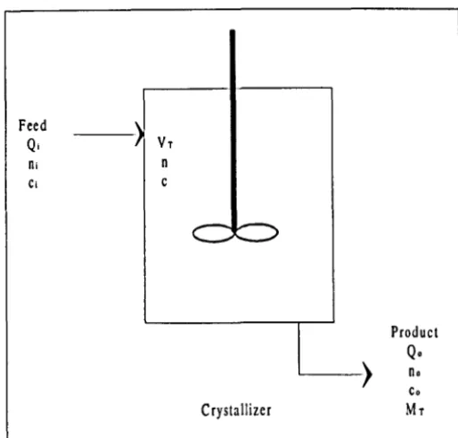
If a well mixed crystallizer Figure (1.2) is considered with a constant slurry volume V_{T ,}it is possible to derive the following partial differential population balance, Randolph and Larson (1988):

(1.47)

In order to simplify this equation, some assumptions can be incorporated: (a)

clear feed (ni

=

0), (b) steady state (on/ch

=

0), (c) G is invariant and (d) a mean

residence time 't is defined as VT/Qo then:

Feed

QI 01

Cl

-)

_Vr 0

C

-~~

Crystallizer

>

Product

Q. o.

c.

Mr

Figure (1.2): Schematic diagram of a simple, perfectly mixed crystallizer.

dn n G - + - = 0

dL

r

( 1.48)

't is also known as the drawdown time, i.e. the time needed to empty the crystallizer

(53)

(1.49)

If the volume of the magma VT, is not constant, then equation (1.47) becomes:

an

+

a

(n G)

+ n

a

(1 n V T )

+

Q 0 n

=

0

at

aL

at

v

T

(1.50)

Equations (1.49) and (1.50) are based on a crystallizer model which is referred to as the mixed-suspension, mixed-product removal (MSMPR) crystallizer, Randolph and Larson (1988). A more general form of the population balance can be given as:

(1.51 )

where Ve and Vi are the external (spatial) and internal particle velocity vectors, respectively and the particle birth and death functions are represented by Band D, respectively. This general form highlights the mathematical similarity with the mass continuity equation (see section 1.3.3) and it is beneficial for spatially distributed systems, as here.

1.1.8. Precipitation Techniques:

In this section, three techniques will be reviewed:

1.1.8a. Precipitation

by

direct mixing

(54)

precipitation happens because the gaseous or liquid phase becomes supersaturated with respect to the solid precipitate. Thus, a crystallization process can be obtained by controlling the degree of supersaturation of a crude precipitation.

Mixing two solutions together as quickly as possible is a common method used to produce a precipitate. A complex analysis, however, may be introduced in some systems. One of the difficulties incorporated in precipitation processes (i.e., highly supersaturated systems) is to obtain uniform conditions throughout the reaction vessel. Consequently, the choice of method of mixing the reactants is of a critical importance to avoid any possible development of excessive supersaturation zones. Also, the development of local pockets of reactants in non-stoichiometric ratios, undesirable pH levels, and so on, can have profound effects.

(55)

1.1.8b. Precipitation From Homogeneous Solution (PFHS)

In general, when gravimetric analysis is aimed, precipitation must be carried out slowly from dilute solution, since an efficient separation of precipitate from liquid is necessary to be affected. Extremely high dilutions and excessively long times, however, are needed for some substances (e.g., hydroxides and basic salts of aluminium, iron and tin) in order to produce dense particles. This method is called "precipitation from homogeneous solution" (PFHS), where coarse precipitates are produced in relatively short times.

PFHS technique can be described as slowly generating the precipitation agent homogeneously within the solution by chemical reaction means. Since the supersaturation levels are under control, undesirable concentration influences are eliminated, a dense granular precipitate is produced and co-precipitation is minimised.

(56)

1.1.8e. Salting-out

This term is assigned for processes where supersaturated solution is obtained with respect to a given solute, by adding a substance that reduces the solubility of the solute in the solvent. The added substance is called "precipitant". The process itself, however, has a variety of other terms such as: watering out, quenching, sol venting out, and so on, depending on the operation involved.

A liquid precipitant needs to be miscible with the solvent of the original solution, at least over the ranges of concentration encountered that the solute be relatively insoluble in it. At the same time, the final solvent-precipitant mixture can be separated (e.g., by distillation), if comprising valuable components.

(57)

Excessive nucleation, in the regions of primary contact, can be avoided by a slight dilution of the salting-out agent with the system solvent. Supersaturation levels (and hence nucleation rates) may also be reduced by the use of diluted precipitant. If the precipitant is a volatile organic liquid, then the procedure can be arranged quite easily.

Not only liquids can be used as precipitant, but also gases and solids, as long as they are miscible in the original solvent without reacting with the solute to be precipitated. Salts can precipitate from solutions by the addition of other crystalline salts, the formation of a stable salt pair is an example of that, Mullin (1993).

1.1.9. Determination of Crystallization Kinetics

In a continuous well-mixed crystallizer under steady state conditions, crystal production rate is identical to the rate of nucleation BO, therefore:

(1.52)

For an MSMPR crystallizer with constant VT:

(1.53) Combining equations (1.49) and (1.53):

B

O

[L ]

n =

a-

exp - G-r (1.54)

(58)

characteristic size, L, on a semi-log paper, gives a straight line with a slope of __ 1_

Or

and an interception of nO = BO/O thereby facilitating simultaneous determination of 0

Since many industrial crystallizers operate in a well-mixed or nearly well-mixed manner, the equations described above can be used to predict their performance. A general correlation of nucleation and growth kinetics, can be obtained by performing a series of runs at different operating conditions. In addition, this correlation can be used to guide either crystallizer scale-up or the development of an operating strategy for an existing crystallizer. Nucleation and growth are influenced by a number of variables such as: temperature, supersaturation, magma density and external stimuli (e.g., agitation or circulation rate of the magma). Usually, empirical power-law functions are used in correlating nucleation and growth rates, but independent variables choice can be obtained from a mechanistic perspective. The following power-law functions are used

quite frequently:

Bo k bM j

= IS T (1.55)

(1.56)

(59)

(1.57)

where k_nis a coefficient, which may depend on process variables such as temperature, rate of agitation or circulation, presence of impurities, and other variables. The system-specific constants i and j can be obtained using experimental data and may be incorporated in scale-up, but noting that j may vary with mixing conditions.

1.1.10. Mass balance constraints

From Figure (1.2), a mass balance on solute can be written as:

(1.58)

where Co is determined by system kinetics and constrained by solid-liquid equilibrium (solubility) relationship, which gives the equilibrium concentration c* at the system conditions. The system is characterised by the supersaturation magnitude (i.e. Co - c*) remaining in the product stream. If the system is closed, where c* is substituted for co, then the system is called a fast-growth or class IT system. On the other hand, if the system is not closed, it is said to be class I (slow-growth) system, where co> c* and

Q.

M = _ I C . - C

T Q

o

I 0 (1.59)

(60)

1.1.11. Moments of crystal size distribution

In this section, the moments equations are derived with a reference to the CSD

section.

The number of crystals, N, up to size L, can be written as:

L

N =

J

ndL (1.60)

o

From equation (1.49):

(1.61 )

This equation is the zeroth moment of the distribution, and as L approaches 00, it

reduced to the total number of crystals in the system:

(1.62)

The first moment of the distribution represents the comulative length (all the crystals laid side by side), but it is not of a critical importance:

L

L =

J

nLdL

o

=

f

noLexp[-~JdL

(61)

(1.63)

ForL -700 : (1.64)

The second moment gives the surface area:

(1.65)

where ka is a surface shape factor. For L -7 00 :

( 1.66)

The third moment gives the mass:

( 1.67)

where kv is a volume shape factor and pc is the crystal density. For L -7 00 :

(1.68)

Dimensionless correlations can be obtained as a single representation of the

above equations using a relative size by putting X=UGt, i.e., the ratio of crystal size to

the size of a crystal that needs a period equals to the residence time 'to

N

- =

N(X)

=

1-exp(-X)

NT

(1.69)

L

- =

L(X)

=

1- (1 + X)exp(-X)

LT

(1.70)

A X2

- = A(X) = 1-(I+X+-)exp(-X)

AT

2

(1.71)

M X2 X3

- = M(X) = l-(1+X+-+-)exp(-X)

A study of reactive precipitation processes using computational fluid dynamics