Electronic Thesis and Dissertation Repository
12-4-2014 12:00 AM
Validation of the multi-segment foot model with bi-planar
Validation of the multi-segment foot model with bi-planar
fluoroscopy
fluoroscopy
Aïda Valevicius
The University of Western Ontario
Supervisor
Dr. Thomas R. Jenkyn
The University of Western Ontario Graduate Program in Kinesiology
A thesis submitted in partial fulfillment of the requirements for the degree in Master of Science © Aïda Valevicius 2014
Follow this and additional works at: https://ir.lib.uwo.ca/etd
Part of the Biomechanics Commons
Recommended Citation Recommended Citation
Valevicius, Aïda, "Validation of the multi-segment foot model with bi-planar fluoroscopy" (2014). Electronic Thesis and Dissertation Repository. 2633.
https://ir.lib.uwo.ca/etd/2633
This Dissertation/Thesis is brought to you for free and open access by Scholarship@Western. It has been accepted for inclusion in Electronic Thesis and Dissertation Repository by an authorized administrator of
VALIDATION OF THE MULTI-SEGMENT FOOT MODEL WITH BI-PLANAR FLUOROSCOPY
(Thesis format: Integrated Article)
by
Aïda Valevicius
Department of Kinesiology Graduate Program in Biomechanics
Submitted in partial fulfillment of the requirements for the degree of
Master of Science – Kinesiology
The School of Graduate and Postdoctoral Studies Western University
London, Ontario, Canada
1 ABSTRACT
A multi-segment foot model (MSFM) is a useful tool for measuring foot joint kinematics
although soft-tissue artefact is often present. Quantifying this error is needed to evaluate
the accuracy of this model. This study validated the MSFM against bi-planar
radiostereometric analysis (RSA) fluoroscopy. Heel-strike, mid-stance, and toe-off
events during the stance phase were compared between motion capture and fluoroscopy.
Rise/drop of the medial longitudinal arch showed a significant difference (p < 0.05)
during toe-off, but no significant difference during heel-strike or mid-stance. Hindfoot
supination/pronation and internal/external rotation, and forefoot supination/pronation
motions showed no significant difference between the two techniques. The lack of
significant difference will allow the MSFM to be used as a sufficiently accurate
technique for measuring foot joint motions.
Keywords: multi-segment foot model, soft-tissue artefact, bi-planar fluoroscopy, RSA,
2 CO-AUTHORSHIP STATEMENT
This work would not have been completed without the help of other people below, whose
help is greatly acknowledged by the author.
Chapter 2: Megan Balsdon designed the study and collected the data.
4 ACKNOWLEDGEMENTS
First I’d like to thank my supervisor Dr. Thomas Jenkyn for guiding me through these
past two years with this project. I got to learn a lot and I appreciate the opportunity I was
given to do this project.
Thanks to the WOBL lab supervisor Ian Jones for helping me set up the cameras and do
the motion capture set-up calibration before every testing period. Also, I need to thank
Lynn Whitred, who very nicely agreed to be my x-ray technician and was a lot of help
during the testing process.
I can’t forget to thank Megan Balsdon for teaching me all there is to know about how to
use the fluoroscopes, calibrate them, process the data, making bone models, matching,
and everything about the fluoroscopy part of this project.
A big thanks to Andrew Dragunas for lending me his video capture equipment so that I
would be able to collect the video feed coming from the fluoroscopes.
Thanks to my friend Lisa Oikawa who helped me along in this entire project; my partner
in crime. I very much appreciated her help for everything going from learning how to
use the hardware and software, to figuring out why things weren’t working, to prepping
the lab for data collection, to getting data collected efficiently. Also, I need to thank her
for being by my side to explore everything that London has to offer, countless runs and
trips to the mall.
I’d like to also thank Daniel Blackburn for being (by default of being my boyfriend) a
great test bunny whenever I needed to practice or try something new out in the lab.
Thanks to by little brother with great artistic skills, much better than mine, for drawing
Thanks to my parents for their support and calmness towards graduate school. I have to
say, rarely to I receive hand written letters in the mail, and usually they only come from
my dad, so here is one that I received from him at some point during my two years in
London. He said it hung in his kitchen during his graduate studies, so then it hung on my
5 TABLE OF CONTENTS
1 ABSTRACT ... ii
2 CO-AUTHORSHIP STATEMENT ... iii
4 ACKNOWLEDGEMENTS ... iv
5 TABLE OF CONTENTS ... vi
6 LIST OF FIGURES ... x
7 LIST OF TABLES ... xvi
8 LIST OF ABBREVIATIONS, SYMBOLS, AND NOMENCLATURE ... xvii
1 CHAPTER 1 – INTRODUCTION ... 1
1.1 Foot Anatomy ... 1
1.1.1 Bones of the Foot ... 1
1.2 Multi-Segment Foot Model ... 3
1.3 Kinematic Measurement Techniques ... 7
1.3.1 Goniometry ... 7
1.3.2 Cinefilm ... 8
1.3.3 Stereophotogrammetry ... 8
1.3.4 Markers ... 9
1.3.5 Soft-tissue artefact ... 10
1.4 Medical Imaging ... 13
1.4.1 X-Ray and Fluoroscopy ... 14
1.4.2 Computed Tomography ... 16
1.5.1 Traditional Radiostereometric Analysis ... 16
1.5.2 Markerless Radiostereometric Analysis ... 17
1.5.3 X-Ray Fluoroscopy ... 20
1.6 Fluoroscopic Calibration ... 22
1.6.1 Pincushion Distortion ... 24
1.6.2 Experimental Setup Recreation ... 28
1.6.3 3D Bone Models ... 29
1.6.4 Matching ... 31
1.7 Rationale ... 33
1.8 Objectives and Hypothesis ... 34
1.9 Thesis Overview ... 35
2 Chapter 2 – Validation of Generic Bone Models for the Use With Bi-Planar RSA Fluoroscopy to Evaluate the Medial Longitudinal Arch ... 36
2.1 Introduction ... 36
2.2 Methods ... 37
2.2.1 Calibration ... 38
2.2.2 Data Collection ... 39
2.2.3 Data processing ... 41
2.3 Results ... 43
2.4 Discussion ... 48
2.5 Conclusion ... 50
3 Chapter 3 – Validation of the Multi-Segment Foot Model against Bi-Planar RSA Fluoroscopy ... 51
3.1 Introduction ... 51
3.2.1 Subjects ... 53
3.2.2 3D-Kinematic Motion Capture Data Collection ... 54
3.2.3 Fluoroscopic Data Collection ... 55
3.2.4 Testing Protocol ... 57
3.2.5 Data Analysis ... 58
3.2.6 Data Analysis – Step 1 – Motion capture data ... 59
3.2.7 Data Analysis – Step 2 – Fluoroscopic data ... 59
3.2.8 Data Analysis – Step 3 – Alignment of Motion Capture and Fluoroscopic Data ... 62
3.2.9 Data Analysis – Step 4 – Statistics ... 63
3.3 Results ... 64
3.4 Discussion ... 80
3.5 Conclusion ... 90
4 Chapter 4 - General Discussion and Conclusions ... 91
4.1 Summary ... 91
4.2 Strengths ... 95
4.3 Limitations ... 96
4.4 Recommendations and Future Directions ... 97
4.5 Significance ... 99
5 References ... 100
6 Appendix ... 109
6.1 Appendix 1 – Cortex Instructions ... 109
6.2 Appendix 2 - Using the Fluoroscopes ... 115
6.3 Appendix 3 – Collection Process ... 119
6.4 Appendix 4 - Bone Segmentation Steps ... 121
6.6 Appendix 6 – Ethics Approval Notice ... 135
6 LIST OF FIGURES
Figure 1-1: Bones of the foot. --- 2
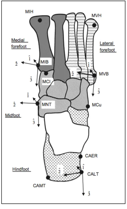
Figure 1-2: Rigid segments of the multi-segment foot model defined as the hindfoot in
dashed grey, midfoot in stripped grey, medial forefoot in solid grey, and lateral
forefoot in tethered grey. The three bony landmarks per segment, which form the
segment-fixed axis systems, are explained in Table 1-1. (Jenkyn & Nicol, 2007) --- 4
Figure 1-3: Joint motions of the MSFM. A) Ankle joint motion defined as the rotation of
the talus with respect to the lower leg segment. B) Subtalar joint motion defined by
the midfoot segment rotation with respect to the talus bone. C) Compound twisting
of the medial and lateral forefoot segments with respect to the midfoot segment. D)
Hindfoot segment motion with respect to the midfoot. E) Shape of the medial
longitudinal arch described as the height-to-length ratio. (Jenkyn & Nicol, 2007) --- 6
Figure 1-4: Calibration frame orientation for bi-planar RSA fluoroscopy. Frame axes x,
y, and z are shown in red, green, and blue respectively. --- 24
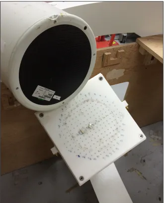
Figure 1-5: Distortion grid attached to fluoroscope B. Known locations of stainless steel
beads embedded in the plastic allow correction for image distortion. --- 26
Figure 1-6: Sample image of distortion grid taken by fluoroscope B. --- 27
Figure 1-7: Close up view of the distortion grid with the numbered beads used for
MATLAB algorithms. --- 27
Figure 1-8: Bone model generation in OsiriX. The red dots correspond to the bony
landmarks that will be used for the study of joint movements with the multi-segment
Figure 1-9: Matching of bones to their respective radiographic images in Rhinoceros
(Rhinoceros, Robert McNeel & Associates, Seattle, WA, USA). --- 33
Figure 2-1: Laboratory set-up with a model foot in position to have fluoroscopic images
taken of the left foot. --- 40
Figure 2-2: Sketch of the bi-planar fluoroscopic RSA set-up (Balsdon, 2011). --- 41
Figure 2-3: Landmarks used to calculate the medial longitudinal arch angle value. Angle
theta is formed by the medial process of the calcaneus, navicular tuberosity, and
distal head of the first metatarsal (Balsdon, 2011). --- 42
Figure 2-4: Medial longitudinal arch (MLA) angle in degrees for each subject across each
condition. --- 47
Figure 2-5: Medial longitudinal arch (MLA) degree angle difference for each generic
condition from the subject-specific condition for all subjects. Values above 0
indicate an overestimation of the MLA angle and values under 0 indicate an
underestimation of the MLA angle. --- 47
Figure 3-1: Location of marker clusters used with the MSFM. Marker clusters are
located on the interphalangeal joint of the hallux, mid-shaft of first and fifth
metatarsals, dorsal to navicular tuberosity, and lateral to Achilles tendon. --- 55
Figure 3-2: Laboratory testing set-up. Subject walking along the custom built wooden
platform while placing her foot in the field of view of the fluoroscopes. --- 58
Figure 3-3: Lateral view of the bones of the foot with red dots indicating exported bony
landmarks. --- 61
Figure 3-4: Medial view of the bones of the foot with red dots indicating exported bony
Figure 3-5: Dorsal view of the metatarsal bones with red dots indicating the exported
bony landmarks. --- 62
Figure 3-6: Hindfoot supination/pronation motion normalized to 0 at quiet standing.
Dashed lines are all the trials calculated using motion-capture and solid lines are
trials calculated using fluoroscopy. Thick dashed and solid lines represent the
average of all trials for motion capture and fluoroscopy, respectively. Trials were
normalized to percentage of stance phase visible using fluoroscopy, 0 representing
heel strike and 100, toe-off. --- 66
Figure 3-7: Hindfoot supination/pronation motion normalized to 0 at quiet standing. The
thick dashed line represents the average of all trials and the thin dashed lines
represent ±1SD for motion capture. The thick solid line represents the average of all
trials and the thin solid lines represent ±1SD for fluoroscopy. --- 67
Figure 3-8: Hindfoot internal/external rotation motion normalized to 0 at quiet standing.
Dashed lines are all the trials calculated using motion-capture and solid lines are
trials calculated using fluoroscopy. Thick dashed and solid lines represent the
average of all trials for motion capture and fluoroscopy, respectively. Trials were
normalized to percentage of stance phase visible using fluoroscopy, 0 representing
heel strike and 100, toe-off. --- 67
Figure 3-9: Hindfoot internal/external rotation motion normalized to 0 at quiet standing.
The thick dashed line represents the average of all trials and the thin dashed lines
represent ±1SD for motion capture. The thick solid line represents the average of all
Figure 3-10: Forefoot angle motion normalized to 0 at quiet standing. Dashed lines are
all the trials calculated using motion-capture and solid lines are trials calculated
using fluoroscopy. Thick dashed and solid lines represent the average of all trials for
motion capture and fluoroscopy, respectively. Trials were normalized to percentage
of stance phase visible using fluoroscopy, 0 representing heel strike and 100, toe-off.
--- 68
Figure 3-11: Forefoot angle motion normalized to 0 at quiet standing. The thick dashed
line represents the average of all trials and the thin dashed lines represent ±1SD for
motion capture. The thick solid line represents the average of all trials and the thin
solid lines represent ±1SD for fluoroscopy. --- 69
Figure 3-12: MLA arch ratio normalized to 0 at quiet standing. Dashed lines are all the
trials calculated using motion capture and solid lines are trials calculated using
fluoroscopy. Thick dashed and solid lines represent the average of all trials for
motion capture and fluoroscopy, respectively. Trials were normalized to percentage
of stance phase visible using fluoroscopy, 0 representing heel strike and 100, toe-off.
--- 69
Figure 3-13: MLA height-to-length ratio normalized to 0 at quiet standing. Thick dashed
line represents the average of all trials and the thin dashed lines represent ±1SD for
motion capture. The thick solid line represents the average of all trials and the thin
solid lines represent ±1SD for fluoroscopy. --- 70
Figure 3-14: Hindfoot Supination/Pronation degree difference between fluoroscopy and
motion capture for both trials from all five subjects. Black cross indicates the
Figure 3-15: Hindfoot internal/external rotation degree difference between fluoroscopy
and motion capture for both trials from all five subjects. Black cross indicates the
average angle difference between both measurement techniques. --- 74
Figure 3-16: Forefoot supination/pronation degree difference between fluoroscopy and
motion capture for both trials from all five subjects. Black cross indicates the
average angle difference between both measurement techniques. --- 75
Figure 3-17: MLA height-to-length ratio value difference between fluoroscopy and
motion capture for both trials from all five subjects. Black cross indicates the
average angle difference between both measurement techniques. --- 76
Figure 3-18: Average supination/pronation motion of the hindfoot at heel-strike,
mid-stance, and toe-off for motion capture and fluoroscopy in stripped and solid grey
respectively. One standard error above and below the mean is indicated by error
bars. --- 78
Figure 3-19: Average internal/external rotation of the hindfoot at heel strike, mid stance,
and toe off for motion capture and fluoroscopy in stripped and solid grey
respectively. One standard error above and below the mean is indicated by error
bars. --- 78
Figure 3-20: Forefoot angle motion at heel strike, mid stance, and toe off for motion
capture and fluoroscopy in stripped and solid grey respectively. One standard error
above and below the mean is indicated by error bars. --- 79
Figure 3-21: Average MLA height-to-length ratio at heel strike, mid stance, and toe off
for motion capture and fluoroscopy in stripped and solid grey respectively. Error
between motion capture and fluoroscopy is indicated by an asterisk (*) with p <
0.05. --- 79
Figure 3-22: Comparison of hindfoot supination/pronation motion between this study and
Jenkyn and Nicol (2007) study. Solid black line indicates the results from Jenkyn
and Nicol (2007) and dashed black line indicates the results from this study. --- 81
Figure 3-23: Comparison of hindfoot internal/external rotation motion between this study
and Jenkyn and Nicol (2007) study. Solid black line indicates the results from
Jenkyn and Nicol (2007) and dashed black line indicates the results from this study.
--- 82
Figure 3-24: Comparison of MLA height-to-length ratio between this study and Jenkyn
and Nicol (2007) study. Solid black line indicates the results from Jenkyn and Nicol
(2007) and dashed black line indicates the results from this study. --- 82
Figure 3-25: Comparison of forefoot supination/pronation motion between this study and
Jenkyn and Nicol (2007) study. Solid black line indicates the results from Jenkyn
7 LIST OF TABLES
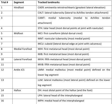
Table 1-1: Name and position of landmarks placed on the bone models ... 30
Table 2-1: Subject anthropometric data ... 38
Table 2-2: Matching conditions for all 5 subjects. Each subject was matched with a 1)
subject-specific bone model (SS), a generic bone models that was of the 2) the
same-size and same-type foot (G_SS_ST), 3) same-same-size and 1st different type foot
(G_SS_DT1), 4) same-size and 2nd different type foot (G_SS_DT2), 5) different-size
and same-type foot (G_DS_ST) ... 44
Table 2-3: Medial longitudinal arch (MLA) angles in degrees for all subjects across all
conditions ... 45
Table 2-4: Difference in degrees between each generic condition and the subject-specific
condition for each subject. The difference is presented as an overestimation
(positive number) or underestimation (negative number). The mean and standard
deviation across all subjects for each condition is also indicated. The average and
standard deviation was calculated based on absolute differences. ... 46
Table 3-1: Subject information data. ... 54
Table 3-2: Average of joint motion values over all trials. The range, maximum, and
minimum values are given in degrees, except for the MLA, for motion capture and
fluoroscopy data. MLA height-to-length ratio is given as a range deviating from 0.
... 64
8 LIST OF ABBREVIATIONS, SYMBOLS, AND
NOMENCLATURE
° - degree(s)
% - percent
2D – two dimensional
3D – three dimensional
3D pose – 3D position and orientation
CAER – calcaneal eminentia retrotrochlearis
CALT – calcaneal lateral tuberosity
CAMT – calcaneal medial tuberosity
Cavus – (pes cavus) participants with high arches
CCD – charge couple device
CMOS – complementary metal oxide semiconductor
CT – computed tomography
d – distance in mm from the fluoroscope source to the image intensifier
DH – distal head of the hallux
fps – frames per second
G_DS_ST – generic different size, same type foot model
G_SS_DT1 – generic same size, different type foot 1 model
G_SS_DT2 – generic same size, different type foot 2 model
G_SS_ST – generic same size, same type foot model
Hz – hertz
ISB – International Society of Biomechanics
LED – light emitting diode
LPH – lateral head of interphalangeal
LLM – lateral malleolus
LMM – medial malleolus
mm – millimeter(s)
mA – milliampere(s)
MCI – first cuneiform
MCU – cuboid
MIB – base of fifth metatarsal
MIH – head of first metatarsal
min - minute
MLA – medial longitudinal arch
MNT – navicular tuberosity
MPH – medial head of interphalangeal
MRI – magnetic resonance imaging
MSFM – multi-segment foot model
ms – millisecond
MVB – base of fifth metatarsal
MVH – head of fifth metatarsal
planus – (pes planus) participants with flat feet or low arches
RSA – radiostereometric analysis
s – second(s)
STA – soft tissue artefact
STC – Standardization and Terminology Committee
STH – talar head
Tiff – tagged image file format
TKA – total knee arthroplasty
μR – micro roentgen
μSv – micro Sievert
WOQIL – Wolf Orthopaedic Quantitative Imaging Laboratory
x-direction – x direction within a coordinate system
y-direction - y direction within a coordinate system
1 CHAPTER 1 – INTRODUCTION
1.1 Foot Anatomy
1.1.1 Bones of the Foot
The foot has the task of giving the body a stable, and efficient interface between the body
and the ground for locomotion. During the gait cycle, the foot has to go from a rigid
lever to allow for push off, to a flexible structure that will allow the foot to adapt to the
ground by absorbing and transmitting forces while keeping whole body stability (Nordin
& Frankel, 2012). The bones, ligaments, tendons, and fascia form joints in the foot that
allow for its vast mobility. The human foot has 26 bones plus 2 sesamoid bones for a
total of 28 bones (Abrahams, 2007). As seen in Figure 1-1, the bones of the hindfoot and
midfoot are the talus, calcaneus, navicular, cuboid, and the three cuneiforms. The
forefoot contains the 5 metatarsal bones and the phalanges. All 5 digits are formed by a
Figure 1-1: Bones of the foot.
There are 6 important joints in the foot that allow for movement to occur. The ankle joint
is formed of the talus and distal parts of the fibula and tibia; it has three dimensional
motion and 6 degrees of freedom. The subtalar joint is formed of the calcaneus and the
talus bone. This joint allows for translations of motion between the tibia and the foot. It
is a hinge joint with an oblique axis, which allows for inversion-eversion and
abduction-adduction motions of the hindfoot. The transverse tarsal joint is made of two joints, the
talonavicular joint and the calcaneocuboid joint. The talonavicular joint is formed of the
talar head and the posterior surface of the navicular. The calcaneonavicular joint is a
saddle joint with not very much motion compared to the talonavicular joint. The
transverse tarsal joint moves as a whole and contributes to pronation and supination of
the foot. The distal intertarsal joints are between the navicular and cuneiform bones,
between the cuboid and lateral cuneiform, and between the three cuneiform bones. These
The tarsometatarsal joints are located between the tarsal bones and the metatarsal bones.
The intermetatarsal joints are between the metatarsals themselves. Their mobility varies
depending of which toe is concerned; the hallux has the most mobility, followed by the
3rd, 4th, and 5th toes. The 2nd toe has limited mobility since it is wedged in between the
cuneiforms and 1st metatarsal base. The metatarsophalangeal joints are the joints
between the metatarsal bones and the phalanges. This joint has its primary motion in the
sagittal plane. Finally, the interphalangeal joints are hinge joints between the phalanges.
Their motion is mostly flexion (Oatis, 2009).
1.2 Multi-Segment Foot Model
Many multi-segment foot models (MSFM) have been developed to quantify
three-dimensional (3D) motions of the joints of the foot. Several models track three foot
segments, the hindfoot (calcaneus and talus), forefoot (metatarsals), and hallux
(phalanges) (Bruening, Cooney, & Buczek, 2012; Carson, Harrington, Thompson,
O'Connor, & Theologis, 2001). Other models incorporate the tibia and fibula as well as
the hindfoot and forefoot (Kidder, Abuzzahab, Harris, & Johnson, 1996; Leardinin,
Benedetti, Catani, Simoncini, & Giannini, 1999; Rattanaprasert, Smith, Sullivan, &
Gilleard, 1999).
Jenkyn and Nicol (2007) developed the MSFM used in this thesis. The model is used for
tracking four segments of the foot. The first segment is the hindfoot and is formed by the
calcaneus. The second segment is the midfoot and is formed by the tarsal bones
including the three cuneiforms, navicular, and cuboid. The third segment is the medial
forefoot consisting of the first and second metatarsals. Finally, the fourth segment is the
represents the different segments of the MSFM as well as the three bony landmarks per
segment, which form the segment fixed axis systems (Jenkyn & Nicol, 2007).
Figure 1-2: Rigid segments of the multi-segment foot model defined as the hindfoot in dashed grey, midfoot in stripped grey, medial forefoot in solid grey, and lateral forefoot in tethered grey. The three bony landmarks per
segment, which form the segment-fixed axis systems, are explained in Table 1-1. (Jenkyn & Nicol, 2007)
There are six foot joint motions defined by Jenkyn and Nicol’s (2007) MSFM, 1) ankle
joint, 2) subtalar joint, 3) hindfoot segment motion with respect to the midfoot in the
frontal plane, 4) hindfoot segment motion with respect to the midfoot in the transverse
plane, 5) forefoot segment motion, and 6) the height-to-length ratio of the medial
The ankle joint motion, also called talocrural motion, is defined as the rotation of the
talus with respect to the lower leg segment about the vector 2-axis of the ankle joint
coordinate system (JCS). A positive rotation about the vector 2-axis is representative of
dorsiflexion as represented in part A of Figure 1-3. The subtalar joint, also called
talocalcaneonavicular joint, motion was defined as midfoot segment rotation with respect
to the talus about the vector 2-axis of the Subtalar-JCS. A positive rotation about the
vector 2-axis is representative of inversion and a negative rotation is eversion of the
midfoot segment as represented in part B of Figure 1-3 (Jenkyn & Nicol, 2007). These
joint motions were defined initially by the Standardization and Terminology Committee
(STC) of the International Society of Biomechanics (ISB). The STC defined the ankle
joint as the articulation between the talus and the tibia/fibula. The subtalar joint was
defined as the articulation between the talus and the calcaneus. From those joint motions,
they defined a JCS for the ankle and subtalar joints (Wu et al., 2002). Hindfoot motion is
presented in part D of Figure 1-3; the movement of the hindfoot with respect to the
midfoot segment is defined as supination/pronation about the midfoot vector 3-axis and
internal/external rotation about the midfoot vector 1-axis. These motions are described in
the method of Grood and Suntay (1983) (Grood & Suntay, 1983). Moving on to the
forefoot, which is presented in part C of Figure 1-3, the compound twisting of the lateral
and medial forefoot segments with respect to the midfoot segment defined the fifth joint
motion of the MSFM. This angle is created between the vector 2-axis of the midfoot and
the vector joining the heads of the first and fifth metatarsals projected onto the midfoot
vector 1- and 2-axis. An increasing angle represented supination of the forefoot (Jenkyn
Figure 1-3: Joint motions of the MSFM. A) Ankle joint motion defined as the rotation of the talus with respect to the lower leg segment. B) Subtalar joint motion defined by the midfoot segment rotation with respect to the
talus bone. C) Compound twisting of the medial and lateral forefoot segments with respect to the midfoot segment. D) Hindfoot segment motion with respect to the midfoot. E) Shape of the medial longitudinal arch
1.3 Kinematic Measurement Techniques
There are several techniques that have been developed to measure kinematics of gait and
human movement. Kinematics is the study of motion of the limbs and joints of the body
irrespective of forces. Movement is described in terms of displacement, velocity, and
acceleration. Displacement is the distance travelled by an object between two locations
as, for example, the displacement of the knee during walking, which goes from 10° at
heel strike to 70° of flexion at toe off, thus creating 60° of angular displacement. The
change in position, or displacement over time is called velocity. Change in linear or
angular velocity over time is acceleration. Most of gait analysis is based on displacement
information. Many factors can affect walking and running patterns such as walking
speed, age, height, weight, strength and flexibility, and aerobic condition (Oatis, 2009).
Kinematic analysis techniques range from goniometers, film cameras,
stereophotogrammetry, medical imaging, and fluoroscopy.
1.3.1 Goniometry
A simple and basic way to measure joint kinematics is using a goniometer. Goniometry
allows one to measure the range of motion of a joint. There are several different types of
goniometers as described by Goodwin et al. (1992). Universal goniometers are easy to
use, but restricted mostly to simple joint movements or static joint positions. Fluid
goniometers are made of a circular clear tube filled with liquid. As the device is rotated
the fluid moves relative to the graduated disk and makes an angle equal to the angular
displacement of the base. This type of goniometer works independently of the center of
contains a strain gauge steel strip placed between two plastic sections. The angular
displacement of the joint is displayed digitally on the display unit. The beginning of the
movement is set to zero and the end of the motion will be displayed as the angle of the
movement (Goodwin, Clark, Deakes, Burdon, & Lawrence, 1992).
1.3.2 Cinefilm
Another technique for kinematic analysis, which has been widely used in research,
requires the use of cameras, cinefilm, and high-speed cameras. High-speed cameras
allow for assessment of activities with velocities and accelerations greater than walking.
These types of cameras do not require any wires and cables attached to the subject, thus
their range of motion is greatly improved and movement is not obstructed. The down
side with this type of motion capture is that each frame needs to be digitized separately,
which requires a great amount of time and effort (Schneck & Bronzino, 2002).
1.3.3 Stereophotogrammetry
Stereophotogrammetric systems such as ELITE and VICON are commonly used for
kinematic analysis. These systems use two or more cameras placed in different locations
covering a specific capture volume. The subject wears reflective markers placed on
specific body landmarks. Each marker has to be seen by two cameras in order for its
location to be collected by the system (Leardinin et al., 1999). Some cameras have LED
rings around the camera lens. These LEDs act like a strobe light and reflect off the
markers. Infrared lights have become commonly used today for optical motion capture
cameras (Roesler, 2011). The infrared light bounces off the markers covered in
retro-reflective tape, is called a passive marker. Another marker system commonly used in
kinematic analysis requires active markers. Active markers are small LED makers that
are placed on the subjects’ bony landmarks. They produce light that is captured by the
camera’s lens. There are advantages to both types of motion capture systems. Active
markers allow for the location of bony landmarks to be known immediately because the
markers are each fired sequentially and therefore the system can immediately determine
the location of each marker. The main disadvantage of active markers is that they require
a system of cables to power the markers. These cables could be intrusive for movement
patterns. As for passive markers, an advantage is that they simply go on the body with
double-sided tape and are not as intrusive to movement. The disadvantage lies in the
post-processing phase, as the researcher is required to identify the markers after testing,
although algorithms have been developed to make this process faster and automatic
(Schneck & Bronzino, 2002).
1.3.4 Markers
Markers are placed on specific bony landmarks either as single units or as a cluster of
connected markers. The 3D coordinates of the markers in the laboratory frame of
reference are the output of data acquisition using the video camera based systems. Each
body segment requires three markers or reference points in order for a body-fixed
coordinate system to be created and to allow for determination of the six-degree of
freedom motions of that body segment. Vector cross products, from unit vectors
connecting specific markers, produce perpendicular vectors to the marker plane. Using
the newly created cross product vector, a segment-fixed coordinate system is created.
shank, allow for the absolute orientation of body segments, or the relative angle between
body segments to be analyzed (Schneck & Bronzino, 2002).
1.3.5 Soft-tissue artefact
Soft-tissue artifact (STA) is defined as the relative movement between the skin markers
and the underlying bone (Dumas, Camomilla, Bonci, Cheze, & Cappozzo, 2014).
Depending on the placement of markers, different factors will contribute to STA. When
markers are placed closer to joints, inertial effects, deformation, and sliding contribute to
STA. Further away from joints, muscular contraction is the main contributor to STA.
Muscular contraction has a frequency content similar to that of bone movement therefore
it is very difficult to distinguish between the two by using any sort of filtering technique
(Leardini, Chiari, Croce, & Cappozzo, 2005).
Many studies measure and evaluate STA. Reinschmidt et al. (1997) determined the STA
for the tibiofemoral and tibiocalcaneal joint motions during walking using a set of
external skin markers. Intracortical Hofmann bone pins were inserted surgically into the
femoral condyle, lateral tibial condyle, and the posterolateral aspect of the calcaneus of
the right leg. Marker triad clusters were attached to the femur, tibia, and calcaneus bone
pins. Single markers were place on the shoe, thigh, and tibia, with six on each segment.
It was concluded that most of the error for knee rotations came from STA at the thigh.
Skin markers are the better option when determining flexion/extension at the tibiofemoral
joint since the error was lower. The STA error was nearly as large as the magnitude of
the real joint motion when trying to determine abduction/adduction and internal/external
rotation at the knee (Reinschmidt et al., 1997). The same researchers looked at STA
agreement between the skin and bone based patterns. On the other hand, the errors
observed for abduction/adduction and internal/external rotation were large, 70% and 64%
respectively relative to the full range of motion. It was concluded that joint motion was
overestimated with the use of skin markers. STA errors at the shank were approximately
5° across all subjects and all rotations, where as errors at the thigh reached values higher
than 10° for internal/external rotation. Errors due to skin movement were higher during
running trials than walking, as would be expected (Reinschmidt, van den Bogert, Nigg,
Lundberg, & Murphy, 1997).
More closely related to this thesis, Westblad et al. (2002), looked at ankle complex
motion during the stance phase of walking. Three markers were attached to the shank,
heel, and forefoot. These were accompanied with Hoffman pins that were inserted into
the tibia, fibula, talus, and calcaneus. Single markers were attached to each pin for the
walking trials. Their results showed that the mean maximal difference was less than 5°
between skin- and bone-based joint rotations. Moreover, the smallest absolute difference
was found for plantar/dorsiflexion movement (Westblad, Hashimoto, Winson, Lundberg,
& Arndt, 2002).
The type of marker used also affects the magnitude of STA. Skin-mounted markers
create larger STA than markers mounted on rigid plates. Cappozzo et al. (1996), tested
patients being treated for femur and tibia fractures. Unilateral external fixation devices
were fixed to the bones, thus permitting a new set of axes, fixator technical frame, to be
created, which would be a rigid body alongside the relevant bone. Additional skin
markers were placed on the skin’s surface on anatomical landmarks; greater trochanter,
fibula. Clusters of three markers were placed on the pelvis and non-instrumented
segments of the lower limb. Results showed that STA could be of magnitudes ranging
from a couple mm up to 40mm. Skin mounted markers placed above anatomical
landmarks showed displacements that were proportional to the angular displacement of
the closest joint. Movement of the greater trochanter marker was affected by motion of
the hip joint for example and the motion of the knee joint mostly affected movement of
the head of the fibula marker. Therefore, this marker placement location is not optimal.
Markers placed on the shank and thigh showed smaller displacements, indicating that this
would be a better marker placement location. Greatest artefact values were seen during
flexion/extension movements, from 6-20° at the femur and 4-10° in the tibia. Also,
different clusters yielded different artefact results (Cappozzo, Catani, Leardini, Benedetti,
& Croce, 1996).
Several conclusions can be drawn in regards to STA. Errors caused by STA are larger
than errors coming from stereophotogrammetry. STA presents systematic and random
errors which are reproducible within, but not among subjects. STA is task dependent, but
tends to be greater in the thigh compared to other lower limb segments (Leardini et al.,
2005).
When markers are formed as clusters, their movement over the underlying bone is
explained by the sum of four different components. These components are translation of
the cluster, rotation of the cluster about the origin of the reference frame (representing the
pose of a deformable marker cluster), the change in size of the cluster, and the change in
cluster shape, also called deformation. All these transformations may be independent of
effect on position/orientation, size, and shape of marker clusters. They defined STA of a
single marker as the local displacement from a reference position fixed in the reference
frame of the analyzed bone. STA at the cluster level was defined as a rigid displacement
or change in position and orientation, a scaling or a change in size, and a deformation of
the cluster. Steel pins were inserted into the iliac crest, proximal third of the right
femoral diaphysis, and anteromedial aspect of the tibia. Each pin had a cluster of four
markers placed on it. Twelve single markers were placed on the anteromedial, anterior
and anterolateral aspects of the right thigh. Maximal hip and knee flexion were produced
to determine STA. All the parameters describing STA saw pronounced variability across
specimens and across clusters. It was found that STA’s were specimen-specific and
cluster-specific. The subject with the greatest thigh mass exhibited the largest STA at the
single marker and cluster level (Grimpampi, Camomilla, Cereatti, de Leva, & Cappozzo,
2013).
Therefore, the location and type of marker, as well as the body composition of the subject
will have an effect on the type and amount of STA observed during kinematic analysis.
1.4 Medical Imaging
In order to overcome problems related to STA, medical imaging techniques such as
magnetic resonance imaging (MRI) and computed tomography (CT) scans may be used
to produce subject-specific kinematic bone models. These techniques benefit the study of
kinematics because they are non-invasive when compared to radiostereometric analysis
(RSA) techniques that use bone embedded tantalum beads. From the scans,
subject-specific kinematic models are made with a joint coordinate system that is based on the
in gait kinematic values using generic bone models and subject-specific MRI bone
models. Full leg MRI images were taken of subjects in supine position. From the MRI
images bony landmarks were identified manually. Results showed that generic bone
models were substantially different from subject-specific bone models. Generic models
systematically introduced significantly increased hip flexion, external hip rotation and
knee flexion over the gait cycle. When MRI images were compared to kinematic
analysis using VICON and reflective markers, smaller differences were found; only hip
flexion was significantly increased as opposed to all three motions when using generic
bone models (Scheys, Desloovere, Spaepen, Suetens, & Jonkers, 2011).
1.4.1 X-Ray and Fluoroscopy
X-rays are produced by applying a large electrical potential difference between an
electron source and a target. Electrons leaving the x-ray source convert their kinetic
energy to electromagnetic energy as they decelerate and interact with a target material.
An external power source provides high voltage to accelerate the electrons. For
diagnostic purposes, the x-ray source is placed on one side of the patient and the detector
is place of the other side of the patient. During x-ray exposure, some x-rays are
differentially attenuated by the anatomical structures of the patients, these are incident
x-rays. Small portions of x-rays pass through the patient and are recorded on the detector,
thereby creating a radiographic image (Bushberg, Seibert, Leidholdt Jr., & Boone, 2012).
Fluoroscopy allows for real-time x-ray viewing of patients with high temporal resolution.
Real-time imaging produces ‘videos’ with 30 frames per second (fps), which coincides
with older analog television frame rates in the USA. Being able to collect video data is
of different parts. Motorized collimators adjust to the field of view or the
source-to-image distance. It also has a detector like other radiographic systems, but it is in the form
of an image intensifier. As fluoroscopy allows for prolonged real-time image capture,
extremely decreased doses of radiation have to be used. Doses may be one thousandths
of that used for traditional radiography. Typical fluoroscopic detector dose ranges from
1µR to 5µR per image. Thus, the image intensifiers used are very sensitive low-noise
detectors in order to detect low radiation signals. There are four components to the image
intensifier: a) a vacuum housing to allow for unimpeded electron flow, b) an input layer
that transforms the incident x-rays into light, c) an electron optics system that takes the
electrons emitted by the input layer and transfers them to the output layer, and d) an
output phosphor that converts the output electrons into a light image. Coupled with the
output layer of the image intensifier, a light-sensitive camera, such as an analog vidicon,
a solid-state charge couple device (CCD) or complementary metal oxide semiconductor
(CMOS) system is needed in order to relay the output image to a video monitor for
viewing purposes (Bushberg et al., 2012).
Continuous fluoroscopic imaging is possible by producing a continuous x-ray beam,
which uses 0.5 to 6mA. Each fluoroscopic image is displayed on a camera for 33ms;
hence any fast motion will be blurred. Pulsed fluoroscopy can counter the blurring of the
image during continuous fluoroscopy. Pulsed fluoroscopy uses x-ray pulses that can be
between 3 and 10ms in length, allowing for viewing of faster movements (Bushberg et
1.4.2 Computed Tomography
Computed tomography has been available for clinical use since the 1970’s. Over the past
50 years the rotation speed of the scanner has increased from a 4.5 min scan to a sub
half-second rotation. Today, a CT scan can collect over 200 images per half-second. A scanner is
composed of a CT gantry, which is the rotating part of the scanner, and a patient table
that is controlled with precise motors to be positioned in the appropriate position for the
scan. Laser lights also help for the proper positioning of the patient inside the bore. The
scanner’s field of view is a circle in the x-y direction, but when extended in the
z-direction, it becomes a cylindrical field of view. Scans are produced by having the x-ray
tube rotate around the patient. Rays from the x-ray source create a fan beam projection
onto detector arrays. Most detector arrays in clinical CT are arranged in an arc relative to
the x-ray tube (Bushberg et al., 2012).
1.5 Radiostereometric Analysis
1.5.1 Traditional Radiostereometric Analysis
Radiostereometric analysis (RSA) comes from two words, photogrammetry and stereo.
Photogrammetry means to obtain a picture that comes from light and stereo means that an
object has the property of being solid, or having three dimensions (Selvik, 1989). Thus
radiostereometric analysis takes measurements from 2D pictures and reconstructs
three-dimensional objects. In 1898, a London radiologist, Davidson, was the first to attempt to
localize bodies with the use of x-rays. He used a x-ray tube that could be moved along a
horizontal scale. Below it, an x-ray plate was placed with two wires extended on top, at
developed and then brought to another machine called the localizer. In the localizer,
there are two silk threads that go from the foci, during the exposures, to the images of the
radiopaque object that was studied. The point in space where the two silk threads
intersect represents the position of the object (Selvik, 1989). Today, RSA is a
computerized system that allows for the precise location of landmarks in the human body
to be known. Instead of using a localizer, modern RSA uses a cage with fiducial and
control points to calculate 3D coordinate systems (Bottner, Nestor, Azzis, Sculco, &
Bostrom, 2005). Since the body doesn’t have well-defined radiopaque landmarks, other
markers need to be used, which are often surgically implanted into the body. The most
common type of marker is a tantalum bead. The beads have a high inertness to body
tissues and have a high absorption of x-rays, which makes them the ideal choice for RSA
(Selvik, 1990).
There are many applications today for RSA. The first use of RSA occurred in 1973,
when Aronson tested three children with delayed growth by implanting tantalum beads in
the growth zone of their fibulas. Since then, multiple joints and areas of the body have
been studied using RSA. Namely, RSA of the craniovertebral joints, shoulder joints,
hand, spine, pelvis, hip, knee, lower extremities, ankle/foot complex, and growth
disorders has been investigated (Selvik, 1990).
1.5.2 Markerless Radiostereometric Analysis
Classic RSA requires the use of tantalum markers to be inserted into bones of study or
implants. This procedure is rather invasive and allows for the study of only a certain
injured population. Thereby the migration of implants is one of the main study areas of
al., 2005). Implants like metal-backed cups for hip arthroplasty and femoral components
in knee arthroplasty often hide the attached markers (Valstar, de Jong, Vrooman, Rozing,
& Reiber, 2001). Tantalum beads may also compromise the strength and integrity of the
implant itself. Thus markerless RSA or model-based RSA techniques have been
developed to overcome the downsides of classic RSA (Hurschler, Seehaus, Emmerich,
Kaptein, & Windhagen, 2009). Computer-aided design data or reverse engineering is
used with this novel technique. Through these techniques, geometric surface models of
prosthetics or bones can be produced. These virtual models can then be matched to the
real contour of the prosthetic or a bone from a stereographic image. Hurschler et al.
(2009) studied the migration of a TKA tibial component, where a manually implanted
prosthetic was compared with a prosthetic implanted with the aid of a kinematic
navigation system. They also compared model based and marker-based RSA techniques.
Using reverse engineering, a computer model of the knee prosthetic was produced. This
model was matched to stereographic images of the prosthetic. Their results showed that
there was high similarity in the results between model-based and marker-based RSA.
The difference in the means between modelbased and markerbased ranged from
-0.08mm to -0.08mm for in-plane translation, -0.14 to 0.14mm for out-of-plane translation,
from -0.80 to 0.74° for out-of-plane rotation, and from -0.21 to 0.22° for in-plane rotation
(Hurschler et al., 2009).
Valstar et al. (2001) tested the accuracy of a model-based RSA technique using phantom
knee prosthetics. Three components of the prosthetics were analyzed, the femoral and
tibial component of an Interax total knee prosthetic and the femoral component of a
embedded into its surface, to which they attached the prosthetic components to the base
as a phantom. The phantom was positioned in seven different poses for each RSA
radiograph. The location of the phantom and the knee implant was analyzed. The
contour of the implant and the phantom were compared and the position of the implant
was determined by minimizing the difference between the detected contour and the
calculated model contour. The Interax component showed large standard deviation for
rotations. The Profix femoral component showed smaller dimensional differences
between the model and actual prosthetic. Moreover, the micromotion results were more
accurate as the micromotion parameters; especially rotations were closer to zero than the
observed parameters for the Interax component. This method of model-based RSA needs
to have improved sensitivity to dimensional tolerances in order to get better accuracy as
so to replace marker-based RSA (Valstar et al., 2001).
As an alternative to making computer-aided models of bones or prosthetics, CT scans
may be used for creating bone models. A 2D-3D image registration method is used to
find the 3D pose of the CT volume. Once this is done, each 2D radiograph can be
matched to the 3D CT for further kinematic analysis. This method was used by Bruin et
al. (2008) to determine scapular positioning with the intention of validating the procedure
against conventional RSA. Image-based RSA was compared with traditional RSA using
a cadaver specimen and a sawbone structure. The results showed that image-based RSA
had high accuracy with migration of below 0.083mm for translations and below 0.021°
for rotations. The maximum standard deviations were smaller than 0.30mm for
1.5.3 X-Ray Fluoroscopy
Going a step ahead of RSA is x-ray fluoroscopy. This method allows for in vivo joint
kinematics to be studied during dynamic weight-bearing activities. Fluoroscopy has
several other benefits; one being that it exposes the patient to less radiation than
traditional RSA. A 20 second protocol will expose the subject to 80 µSv of radiation
(Ackland, Keynejad, & Pandy, 2011). Most C-arm fluoroscopy units sample at 25 fps,
which is adequate for studying walking or dynamic motions of different joints. Some
devices are able to capture at frame rates up of 250 fps, which allows for high-speed
analysis for motions such as running, jumping, or cycling (You, Siy, Anderst, &
Tashman, 2001). X-Ray fluoroscopy has been used to measure kinematics of the
glenohumeral joint (Fox, Kedgley, Lalone, Johnson, & Athwal, 2011), hip joint (Ioppolo
et al., 2007; Tsai et al., 2013), femur (Baka et al., 2012; Hurvitz & Joskowicz, 2008),
knee (Acker et al., 2011; Banks & Hodge, 1996; Ioppolo et al., 2007; Li, Van de Velde,
Samuel K., & Bingham, 2008; Tersi, Barré, Fantozzi, & Stagni, 2013), ankle and foot
(Martin et al., 2012). Most x-ray fluoroscopy analysis is done by single-plane or
dual-plane. Single-plane fluoroscopy allows for determination of motions with six
degrees-of-freedom (three for translation and three for rotation), but shows rather large out-of-plane
motion errors. Accuracy is increased when using dual-plane fluoroscopy; nonetheless,
single-plane is a useful and a valid way to measure joint kinematics (Ackland et al.,
2011). Acker et al. (2011) used single-plane fluoroscopy and determined its accuracy by
comparing it to optical motion tracking. Knee joint kinematics showed absolute mean
differences between both methods of 2.1°, 0.3°, and 1.1° in extension, abduction, and
translations respectively (Acker et al., 2011). Similarly, Banks et al. (1996) measured the
accuracy of single-plane fluoroscopy on knee replacement kinematics and found that
knee rotations could be measured to the accuracy of 1° and knee translations could be
measured with an accuracy of about 0.5mm. Their method for measuring accuracy was
different, relative poses of implant components against the radiograph were measured and
accuracy was determined as the estimate pose relative to a modeled pose (Banks &
Hodge, 1996).
Tersi et al. (2013) compared the accuracy of single-plane and bi-plane fluoroscopy. They
performed their analysis on dynamic movements of the tibiofemoral joint. Using the
same movements for both fluoroscopic techniques, they validated them against dynamic
fluoroscopic marker-based RSA, which is considered the gold standard. A sawbone
model of the knee joint was made with four tantalum beads embedded in it. Five
repetitions of 10s were performed for three motions, absolute pose kinematics for each
bone segments were calculated for single-plane, bi-planar 3D fluoroscopy, and RSA.
Their results showed that for single-plane fluoroscopy, when calculating in-plane pose
parameters, un-biased and low dispersion pose estimates could be obtained. The errors
for in plane pose parameters were of the same magnitude for single-plane and dual-plane
fluoroscopy. Magnitude of translational errors was less than 0.5mm for single-plane and
0.3mm for dual-plane. Whereas, rotation error was two fold for single-plane compared to
1.6 Fluoroscopic Calibration
When placing two fluoroscopic devices in a laboratory setting, their specific location will
have to be known for data analysis. Laboratory coordinate systems have to be
determined in order to track the movement of specific anatomical landmarks and joints of
interest. Calibration frames have been developed in order to achieve this. Calibration
frames have two sets of planes, control and fiducial. The fiducial plane is used to
transform the image coordinate system to the laboratory coordinate system. The control
plane is used to determine the focal point from which the x-rays originate (Kedgley &
Jenkyn, 2009). Most often bi-planar fluoroscopy is used with the fluoroscopes being
placed at 90° angle relative to each other. With this arrangement, calibration boxes have
been developed in the shape of cubes (Valstar et al., 2005).
This thesis does not place the fluoroscopes at 90°. A non-traditional orientation was
chosen in order to get the best view of a joint or anatomical structure. Placing C-arm
fluoroscopes at 90° relative to each other is very restricting for the study of movement of
joints. Kedgley and Jenkyn (2009) assessed the accuracy of RSA when imaging devices
were placed in a non-traditional orientation. They used both an orthogonal calibration
frame (where the fiducial and control planes were oriented 90° relative to each other) and
a calibration frame where fiducial and control planes were oriented at an angle greater
than 90°. A calibration frame was constructed from an acrylic sheet with each fiducial
and control planes embedded with 45 beads in a 9-bead by 5-bead matrix. Control and
fiducial planes could be set to be at 90°, 105°, 120°, and 135° relative to each other. The
use of an angled calibration frame did not improve the accuracy of the overall calibration
135°, the use of the calibration frame at 90° showed equivalent or better accuracy than
when the fluoroscopes were positioned at right angles. Greatest accuracy values were in
the range of 90.0±24.0μm for calibration frame and fluoroscopes placed at 105° and
lowest accuracy was found with a 135° position having magnitudes of 227.2±120.9μm.
Accuracy for a 90° calibration frame and fluoroscope placement fell between these two
values. Thus, RSA imaging can be performed with the devices being placed at relative
angle to each other of other than 90° with proper accuracy (Kedgley & Jenkyn, 2009).
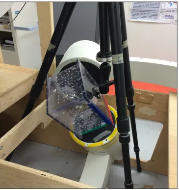
Figure 1-4 is an example of how the fluoroscopes and calibration frame is placed in this
Figure 1-4: Calibration frame orientation for bi-planar RSA fluoroscopy. Frame axes x, y, and z are shown in red, green, and blue respectively.
1.6.1 Pincushion Distortion
Fluoroscopic analysis may cause extensive spatial distortion of radiographic images
(Wearing et al., 2005). Types of distortions that may occur are pincushion distortion,
shading, veiling glare, characteristic curve, and de bias. Pincushion distortion is the most
significant cause of spacial non-linearity. It is caused by the combination of a curved
non-uniform magnification of the peripheral aspect of the image (Boone, Seibert, Barrett, &
Blood, 1991).
Distortion is most often corrected with a grid of beads or wires that is placed in front of
the image intensifier to quantify the amount of distortion that is present. There are
several ways to correct for distortion. Local distortion correction algorithms use three or
four points that surround a small area of an image and correct for that area. Global
distortion correction algorithms use the coordinates of as many grid points as can be seen
in the image and calculate a distortion vector at each point. Positions of the beads in the
image are related to the known positions of the beads according to a polynomial. Global
distortion correction was found to be superior to local distortion correction techniques as
it is not only considerably faster, but it also has less digitization error than local distortion
as it is removed by using a least-squares fit method (Gronenschild, 1997). After each
testing procedure during this thesis, pincushion distortion had to be assessed. The
technique used was the one previously developed in the lab by Kedgley et al. (2012). A
grid made of a 9.5mm thick Delrin sheet with 131 2-diameter stainless steel beads spaced
apart by 15mm was used (Figure 1-5 and 1-7). The positions of the beads were
determined using a coordinate measuring machine. After a testing session, the grid was
attached to each image intensifier and an image with the position of the beads was
collected. The position of each bead was located manually using a custom-written
algorithm in MATLAB (Figure 1-6). A range of polynomials was used for distortion
correction, from first degree in each direction (second order polynomial) to third degree
in each direction (sixth order polynomial). Kedgley et al. (2012) found that a fourth
direction polynomial fit. They also found that image distortion is most important for 2D
analysis. The use of a calibration frame for 3D analysis tempers the effects of distortion,
which lead to accuracies in the RSA reconstruction with uncorrected points that were
much better than anticipated. The error in RSA reconstruction of uncorrected points was
found to be 192±68µm (Kedgley, Fox, & Jenkyn, 2012).
Figure 1-6: Sample image of distortion grid taken by fluoroscope B.
1.6.2 Experimental Setup Recreation
Through the use of MATLAB algorithms (The MathWorks; Natick, MA, USA) the x-ray
source positions, the orientation and location of the image plane with respect to the x-ray
source were determined. This was done by determining and optimizing three Euler angle
rotations and the distance ‘d’ from the source to the image plane. Once the fluoroscopic
parameters are determined, the experimental set-up can be recreated in solid modeling
software Rhinoceros (Rhinoceros, Robert McNeel & Associates, Seattle, WA, USA).
The virtual set-up allows for the import of bone models that will be matched to the
fluoroscopic images. The set-up was done following the instructions from Appendix E
and F from Anne-Marie Allen’s thesis (2009). The first step orients the fluoroscopic
coordinate system in the correct orientation. A point for the x-ray source is recreated
using the x-ray source coordinates that were found by running the MATLAB algorithms.
A vector of length ‘d’ is created from the last rotation of the fluoroscope coordinate
system. The vector is linked to the x-ray source and an image plane orthogonal to the
vector is created and is coincident with the other end of the ‘d’ vector. The image plane
is formed according to the known size of the fluoroscopic images (540x720 pixels). The
fluoroscopic calibration images are imported into the image plane as are the 2D
distortion-corrected fiducial and control points. These points have to be aligned with the
3D calibration frame points for the final image plane correction. Each fluoroscope
calibration is done separately and then one is imported into the other in order to have a
1.6.3 3D Bone Models
3D bone models have to be imported into the recreated lab set-up to be matched to the
fluoroscopic images in this thesis. The bone-models used for the second chapter of this
thesis are subject-specific bone models, which were created from CT scans of the tested
subjects. The bone models used in the third chapter of this study were taken from a bank
of ‘generic’ CT scans and matched to the subject’s foot by size.
The CT scans are converted into bone models in an open source image processing and
DICOM viewing software OsiriX (Pixmeo, Geneva, Switzerland). Bone segmentation
step-by-step instructions are presented in Appendix 4. Each bone of interest is segmented
individually in order to be imported into Rhinoceros for matching. The 3D Volume
Rendering window allows for segmentation and isolation of each individual bone using
specific tools. It is during this part of bone model creation that the bony landmarks are
placed on the bones (Figure 1-8). The bony landmarks used in the third chapter of this
Table 1-1: Name and position of landmarks placed on the bone models
Trial # Segment Tracked landmarks
1 Hindfoot CAER: eminentia retrotrochlearis (greatest lateral elevation) 2 CALT: lateral tuberosity (lateral to Achilles tendon attachment) 3 CAMT: medial tuberosity (medial to Achilles tendon
attachment)
4 STH: talar head (most dorsal points at joint with navicular) 5 Midfoot MCI: first cuneiform (distal dorsal crest)
6 MNT: navicular tuberosity (most medial point)
7 MCU: cuboid (lateral dorsal edge at joint with calcaneus) 8 Medial Forefoot MIH: first metatarsal head (most dorsal point)
9 MIB: first metatarsal base (most dorsal point) 10 Lateral Forefoot MVH: fifth metatarsal head (most dorsal point) 11 MVB: fifth metatarsal base (most dorsal point)
12 Ankle JCS LMM: medial malleolus (most medial point) defined on the lower leg segment
13 LLM: lateral malleolus (most lateral point) defined on the lower leg segment
14 Hallux DH: most distal point of the hallux (and the foot) 15 LPH: lateral head of the interphalangeal