`
ABSTRACT
LIU YANG. Development of a Data-Driven Analysis Framework for Boiling Problems with Multiphase-CFD Solver (Under the direction of Dr. Nam Dinh).
Flow boiling is a highly efficient heat transfer regime, which is used for thermal management in various engineered systems. Among the modeling tools for boiling, the Multiphase Computational Fluid Dynamics (MCFD) solver based on Eulerian-Eulerian two-fluid model has demonstrated its potential in solving boiling problems for industrial applications. On the other hand, in two-fluid model, closure relations are needed to make the two-fluid conservation equations solvable. Such relations, usually empirical or semi-empirical correlations, bring model form uncertainty and model parameter uncertainty to the MCFD solver. A still open issue for MCFD is that such uncertainties can be significant and are still not well quantified, thus undermining the predictive capability of the solver.
This dissertation presents a data-driven analysis framework to address this open issue. The framework aims to leverage state of the art statistical methods and the increasingly affluent boiling data, from both high-resolution experimental measurements and high-fidelity simulations, to 1). perform validation and uncertainty quantification (VUQ) for the MCFD solver based on all available datasets; 2). develop data-driven closure relations based on deep neural networks for the MCFD solver that has the better predictive capability. Three major products are developed within the framework.
`
`
Development of a Data-Driven Analysis Framework for Boiling Problems with Multiphase-CFD Solver
by Yang Liu
A dissertation submitted to the Graduate Faculty of North Carolina State University
in partial fulfillment of the requirements for the degree of
Doctor of Philosophy
Nuclear Engineering
Raleigh, North Carolina 2018
APPROVED BY:
_______________________________ _______________________________ Dr. Nam Dinh Dr. Ralph Smith
Committee Chair
ii DEDICATION
iii BIOGRAPHY
Yang Liu was born in China, Hunan province. He was educated through high school in his hometown. He obtained his college education at Tsinghua University in Beijing, from where he received his bachelor’s degree in nuclear engineering in 2010. After that, he obtained his master’s degree in nuclear engineering from China Institute of Atomic Energy in 2013.
iv ACKNOWLEDGMENTS
The work presented in this dissertation is the outcome of a challenging yet rewarding intellectual experience. First, I would like to thank my advisor, Professor Nam Dinh, for his encouragement, support, and guidance during the course of this research. He lighted up the path towards the idea of data-driven approach for me. He also pushed me to become a more disciplined thinker. I’m truly grateful for the freedom he gave me to explore the specific projects in which I found interest. He has been and will always be a role model for me.
I would also like to express my gratitude to my dissertation committee, Professor Ralph Smith, Professor Joseph Doster, and Professor Igor Bolotnov. They have contributed many insightful perspectives for which I deeply value as a crucial part of my graduate experience.
I owe a great debt of gratitude to Carolyn Coyle and Professor Jacopo Buongiorno (Massachusetts Institute of Technology) who provided their high-quality boiling data, and to Dr. Yohei Sato and Dr. Bojan Niceno (Paul Scherrer Institute) who provided their high-fidelity simulation results. Without the data they provided, this data-driven analysis framework would become a castle in the air.
My work would not have been possible without the financial support from the Consortium for Advanced Simulation of Light Water Reactors (CASL).
v TABLE OF CONTENTS
LIST OF TABLES ... viii
LIST OF FIGURES ... ix
NOMENCLATURE ... xii
CHAPTER 1. INTRODUCTION ... 1
1.1 Background ... 1
1.2 Motivation ... 6
1.3 Dissertation overview and outline ... 8
CHAPTER 2. OVERVIEW OF THE PROPOSED FRAMEWORK ... 10
2.1 Essential concepts ... 10
2.1.1 Verification ... 10
2.1.2 Validation ... 11
2.1.3 Sources of uncertainty... 11
2.1.4 Uncertainty quantification ... 12
2.1.5 Sensitivity analysis... 13
2.1.6 Predictive capability... 13
2.1.7 Data-driven modeling ... 14
2.2 Overview of the proposed framework ... 14
CHAPTER 3. DATA PROCESSING AND STORAGE ... 17
3.1 Processing boiling images from IR camera ... 17
3.1.1 Heat flux distribution processing ... 19
3.1.2 Nucleation information processing ... 20
3.2 Processing high-fidelity simulation results ... 23
3.3 “Virtual container” for data storage ... 26
vi CHAPTER 4. METHODOLOGY DEVELOPMENT FOR THE VALIDATION AND
UNCERTAINTY QUANTIFICATION FOR MCFD SOLVER ... 29
4.1 Eulerian-Eulerian two-fluid model based MCFD solver ... 29
4.1.1 Conservative equations ... 29
4.1.2 Characterization of closure relations in MCFD ... 30
4.1.3 Characterization of uncertainties of MCFD solver ... 39
4.2 VUQ procedure for MCFD solver ... 41
4.2.1 First step: solver evaluation and data collection ... 45
4.2.2 Second step: surrogate construction... 46
4.2.3 Third step: sensitivity analysis ... 50
4.2.4 Fourth step: parameter selection ... 55
4.2.5 Fifth step: Uncertainty quantification ... 58
4.2.6 Sixth step: validation metrics ... 61
4.3 Summary remarks ... 63
CHAPTER.5 CASE STUDIES OF THE PROPOSED VALIDATION AND UNCERTAINTY QUANTIFICATION PROCEDURE ... 65
5.1 Case Study I: VUQ on wall boiling heat transfer ... 66
5.1.1 Solver evaluation and data collection ... 66
5.1.2 Surrogate construction ... 70
5.1.3 Sensitivity analysis... 71
5.1.4 Parameter selection ... 73
5.1.5 Uncertainty quantification ... 74
5.1.6 Validation metrics ... 80
5.2 Case study II: VUQ on flow dynamics ... 83
5.2.1 Solver evaluation and data collection ... 83
vii
5.2.3 Sensitivity analysis... 90
5.2.4 Uncertainty quantification ... 91
5.2.5 Validation metrics ... 97
5.3 Summary remarks ... 99
CHAPTER 6. DATA DRIVEN MODELING OF BOILING HEAT TRANSFER ... 102
6.1 Fundamentals of deep learning ... 102
6.2 Problem setup... 108
6.3 Results and discussions ... 113
6.4 Summary remarks ... 122
CHAPTER 7. CONCLUSIONS ... 123
7.1 Summary ... 123
7.2 Contributions... 124
7.3 Future work ... 126
viii LIST OF TABLES
Table 1. Example of an experimental data container. ... 27
Table 2. Expressions of interfacial forces. ... 34
Table 3. Selected models for nucleation site density. ... 37
Table 4. Selected models for bubble departure diameter. ... 37
Table 5. Selected models for bubble departure frequency. ... 38
Table 6. Summary of evaluations for wall boiling heat transfer scenario. ... 67
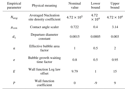
Table 7. Prior uncertainties of studied empirical parameters in wall boiling closure relations. ... 70
Table 8. Optimal selection scores for different QoIs. ... 74
Table 9. Boiling datasets decomposition for different purposes. ... 75
Table 10.posterior statistics of selected empirical parameters. ... 78
Table 11. Summary of evaluations for interfacial momentum closure relations. ... 84
Table 12. Summary of the studied interfacial momentum closure relations. ... 85
Table 13. Prior uncertainties of parameters in interfacial momentum closure relations. . 85
Table 14. Cross validation results. ... 89
Table 15. Flow dynamics datasets decomposition for different purposes. ... 92
Table 16. Summary of posterior distributions of the influential interfacial force coefficients. ... 94
Table 17. Summary of input features of DNN ... 112
Table 18. Outputs of DFNN... 113
Table 19. Case studies based on different training/testing data decomposition ... 114
ix LIST OF FIGURES
Figure 1. Validation hierarchy for MCFD solver based on AIAA guidance ... 4
Figure 2. Overview of the data-driven analysis framework ... 15
Figure 3. Schematic of measuring high-resolution boiling process with IR camera ... 18
Figure 4. Automatic data processing for IR boiling images ... 18
Figure 5. Scheme of computational domain for deriving heat flux distribution on heating surface ... 19
Figure 6. Three frames of (1) appearance of hot spot (t = 0ms); (2) Some hot spots being rewetted while others beginning merging (t = 60.3 ms); (3) Merged hot spot become irreversible and lead to burnout (t = 119.7 ms); 𝑞 = 2.15 𝑀𝑊/𝑚2, BETA experiment ... 19
Figure 7. Temperature and corresponding heat flux distribution in flow boiling, mass flow rate = 500kg/m2, heat flux = 1.4MW/m2 ... 20
Figure 8. Example of hierarchical clustering for active nucleation sites identification .... 22
Figure 9. Evaporation Heat Flux and Bubble Area Fraction Distributions, 𝑞 = 1.16 MW/m2, BETA experiment, Heater Ti36A ... 23
Figure 10. Demonstration of the average process, from bubble interface to void fraction ... 25
Figure 11. Collaboration between two virtual containers ... 28
Figure 12. Closure relation structures in a typical MCFD solver ... 32
Figure 13. Schemes of interfacial forces... 33
Figure 14. Illustration of heat partitioning in (a).” Generation-I” boiling model; (b).Refined boiling models; (c). Boiling model for DNB prediction ... 38
Figure 15. VUQ relationship of MCFD solver, closure relations, and data under TDMI approach ... 42
Figure 16. Two different validation paradigms: (a) Traditional validation; (b)VUQ based on total data-model integration ... 43
Figure 17. Workflow of the proposed VUQ procedure ... 44
Figure 18. Evaluation of model form uncertainty and model parameter uncertainty ... 60
Figure 19. Example of area metric ... 63
x
Figure 21. Structure of wall boiling closures in this case study ... 71
Figure 22. Morris screening measures for wall boiling empirical parameters ... 72
Figure 23. Sobol indices for wall boiling empirical parameters ... 73
Figure 24. Model form uncertainty 𝛿(𝑞𝑤𝑎𝑙𝑙) for different QoIs ... 75
Figure 25. MCMC sample traces and auto-correlations of wall boiling closure relation parameters ... 77
Figure 26. Marginal and pair-wise joint distributions of selected empirical parameters.. 78
Figure 27. 95% confidence intervals (CIs) for different QoIs from wall boiling closure relations ... 79
Figure 28. Confidence intervals for different QoIs from wall boiling closure relations .. 80
Figure 29. Area metrics for different QoIs from wall boiling closure relations ... 82
Figure 30. Accumulative percentage of variances explained by PCs ... 86
Figure 31. Variations of two QoIs captured by 8 PCs (𝑗𝑔 = 0.29 m/s, 𝑗𝑙 = 1.1 m/s)... 87
Figure 32. Comparison of PC scores between MCFD simulations and GP predictions ... 88
Figure 33. Morris screening measures for interfacial force coefficients ... 90
Figure 34. Sobol indices for interfacial force coefficients ... 91
Figure 35. Model form uncertainty distribution at r/R = 0.55 ... 92
Figure 36. MCMC sample traces and auto-correlations of selected interfacial force coefficients ... 93
Figure 37. Marginal and pair-wise joint distributions of selected interfacial force coefficients ... 94
Figure 38. 95% confidence intervals of QoIs for model form uncertainty evaluation cases (first row: 𝑗𝑔 = 0.16 m/s, 𝑗𝑙 = 0.64 m/s; second row: 𝑗𝑔 = 0.09 m/s, 𝑗𝑙 = 2.0 m/s; third row: 𝑗𝑔 = 0.16 m/s, 𝑗𝑙 = 2.0 m/s; fuorth row: 𝑗𝑔 = 0.48 m/s, 𝑗𝑙 = 2.0 m/s) ... 95
Figure 39. 95% confidence intervals of QoIs for model parameter uncertainty evaluation cases (first row: 𝑗𝑔 = 0.09 m/s, 𝑗𝑙 = 0.64 m/s; second row: 𝑗𝑔 = 0.29 m/s, 𝑗𝑙= 1.1 m/s; third row: 𝑗𝑔 = 0.29 m/s, 𝑗𝑙 = 2.0 m/s) ... 96
xi Figure 41. Confidence intervals for three representative cases (first row:
𝑗𝑔 = 0.09 m/s, 𝑗𝑙 = 0.64 m/s; second row: 𝑗𝑔 = 0.16 m/s, 𝑗𝑙 = 0.64 m/s;
third row: 𝑗𝑔 = 0.09 m/s, 𝑗𝑙 = 1.1 m/s) ... 97
Figure 42. Area metrics for three representative cases (first row: 𝑗𝑔= 0.09 m/s, 𝑗𝑙 = 0.64 m/s; second row: 𝑗𝑔 = 0.16 m/s, 𝑗𝑙 = 0.64 m/s; third row: 𝑗𝑔 = 0.09 m/s, 𝑗𝑙 = 1.1 m/s) ... 98
Figure 43. Architecture of a fully connected deep feedforward network ... 103
Figure 44. Demonstration of (a) forward-propagation of input features; (b) back-propagation of loss function gradients ... 105
Figure 45. Computational domain and data sampling area of the ITM simulations... 109
Figure 46. Histogram of 4 QoIs on different input heat fluxes ... 111
Figure 47. Architecture of DFNN used for predicting boiling heat transfer ... 113
Figure 48. Demonstrating of hyperparameter influence on DFNN performance ... 115
Figure 49. Comparison of DFNN predictions and real ITM simulations (Case 2)... 117
Figure 50. Comparison of DFNN predictions and real ITM simulations (Case 3)... 117
Figure 51. Comparison of DFNN predictions and real ITM simulations (Case 1)... 118
Figure 52. Comparison of DFNN predictions and real ITM simulations (Case 4)... 118
Figure 53. Visual comparison of DFNN predictions and ITM results (Case 2) ... 121
xii NOMENCLATURE
𝑎 effective bubble area factor 𝐴𝑎 interfacial area concentration, 1/m 𝐴𝑏 effective bubble area fraction C𝑑 drag coefficient
C𝑙 lift coefficient
C𝑤𝑙 wall lubrication coefficient
C𝑝 specific heat at constant pressure, J/(kg∙K) C𝑣𝑚 virtual mass coefficient
𝐷𝑑 bubble departure diameter, m 𝐷𝑆 bubble diameter in bulk flow, m 𝑑1 departure diameter constant, m/rad
𝑒 bubble growth waiting time factor 𝐸 turbulence wall function Log law offset 𝑓𝑑 bubble departure frequency, 1/s
𝒈 Gravity vector, m/s2 ℎ specific enthalpy, J/kg
ℎ𝑓𝑔 latent heat of evaporation, J/kg
ℎ𝑙 forced convective heat transfer coefficient, W/(m2∙K) ℎ𝑙𝑔 interfacial heat transfer coefficient, W/(m2∙K)
𝑴 interfacial force, N/m3 𝑁𝑎 nucleation site density, 1/m2
𝑁𝑎𝑣𝑔 averaged Nucleation site density coefficient, 1/m2 𝒏𝒘 unit vector normal to the wall
𝑃𝑟𝑡 turbulent Prandtl number
𝑝 pressure, Pa
𝑞𝑤𝑎𝑙𝑙 wall heat flux, W/m2
𝑞𝐸𝑣 evaporation heat flux, W/m2 𝑞𝑄𝑢 quenching heat flux, W/m2
𝑞𝐹𝑐 forced convective heat flux, W/m2
𝑇 temperature, K
𝑡 time, s
𝑼 velocity, m/s
xiii 𝑦+ dimensionless wall distance
𝐴𝑎 interfacial area concentration, 1/m 𝐴𝑏 effective bubble area fraction C𝑑 drag coefficient
C𝑙 lift coefficient
C𝑤𝑙 wall lubrication coefficient
C𝑝 specific heat at constant pressure, J/(kg∙K) C𝑣𝑚 virtual mass coefficient
𝐷𝑑 bubble departure diameter, m 𝐷𝑆 bubble diameter in bulk flow, m
𝑓𝑑 bubble departure frequency, 1/s 𝒈 gravity vector, m/s2
ℎ specific enthalpy, J/kg
ℎ𝑓𝑔 latent heat of evaporation, J/kg
ℎ𝑙 forced convective heat transfer coefficient, W/(m2∙K) ℎ𝑙𝑔 interfacial heat transfer coefficient, W/(m2∙K)
𝑴 interfacial force, N/m3 Greek symbols
𝛼 void fraction
𝛤𝑘𝑖 evaporation/condensation rate per volume, kg/(m3∙s) 𝜃 contact angle, rad
𝜎 surface tension, kg/s2
𝜎𝑡 turbulent dispersion coefficient
κ von Karman constant
𝜆 thermal conductivity, W/(m∙K) 𝜇 dynamic viscosity, Pa∙s
𝜇𝑐𝑜𝑛 contact angle scaler, 1/rad 𝜐 kinematic viscosity, m2/s
𝜌 density, kg/m3
𝜏 stress tensor, kg/(m∙s2)
Φ source term of interfacial area concentration, 1/m3 Subscript
xiv
𝑟 relative motion
𝑠𝑎𝑡 saturation
𝑠𝑢𝑏 subcooling
𝑠𝑢𝑝 superheat
𝑙 liquid phase
Superscript
𝑡 turbulence
1 CHAPTER 1. INTRODUCTION
1.1 Background
Two-phase flow and boiling heat transfer occurs in many situations and are used for thermal management in various engineered systems with high energy density, from power electronics to heat exchangers in power plants and nuclear reactors. Essentially, two-phase and boiling heat transfer is a complex multiphysics process, which involves different interactions between heated solid surface, liquid, and vapor, including nucleation, evaporation, condensation, interfacial mass/heat/momentum exchange, and interface topological change (such as bubble breakup or coalescence). Correspondingly, there are various quantities of interest (QoIs) of a given boiling system, such as flow pattern, pressure drop, wall heat transfer, void fraction distribution, phasic temperature and velocity distribution, etc. In nuclear engineering, understanding the relevant phenomena and accurately predicting the QoIs involve in two-phase flow and boiling heat transfer is crucial for the design of an efficient and safe reactor.
The measurement of many phenomena related to two-phase flow and boiling heat transfer is very challenging with current experimental techniques. Moreover, the experimental study of two-phase flow and boiling at prototypical reactor scale is technically challenging and expensive. Thus in current practices, the design and safety analysis of reactor thermal hydraulics systems are highly dependent on the scientific modeling and simulation.
The modeling of two-phase flow and boiling heat transfer for engineering purpose can be characterized by two aspects: the dimension and the treatment of interfacial interaction. The system code, such as TRACE [1] and COBRA-TF [2] deals with one-dimension cross-sectional averaged problems, while multiphase computational fluid dynamics (MCFD) code deals with multi-dimensional problems. The treatment of interfacial interaction has two types: the mixture model and the Eulerian-Eulerian two-fluid model.
2 energy is needed. The mixture model is further divided, based on their treatment of mechanical non-equilibrium (the relative velocity between the two phases). The homogeneous equilibrium model assumes there is no relative velocity between the phases. The slip factor model uses empirical correlations for the slip ratio (which is defined by the ratio of vapor velocity to liquid velocity). The drift-flux model uses kinematic constitutive equations to describe the relative flow. Theoretically, all three models can be applied to both one-dimension cross-sectional averaged problem and multi-dimensional problems. In practice, however, these models are mainly used for one-dimension cross-sectional averaged problems, such as in system analysis and engineering calculations.
The two-fluid model treats two phases by separate sets of field conservation equations. For one-dimension cross-sectional averaged formulation, the interfacial interactions are modeled in a correspondingly coarse manner. Notably, the effect of local interactions, e.g., wall boiling heat transfer, is coarsened as a source term that affects the cross-sectional averaged parameters of flow dynamics. In contrast, the multi-dimensional formulation requires a much larger set of closure relations needed to provide detailed modeling of interfacial interactions and wall heat transfer.
There are two common features of those modeling approaches: 1). the interface between two phases is averaged and is not resolved in the simulation; 2). closure relations are required to make the conservation equations of the model solvable. Among those approaches, the MCFD solver based on Eulerian-Eulerian two-fluid model has been regarded as the most promising tool, especially for applications with complex geometries such as reactor fuel rod bundles. The main reason is MCFD has the capability to describe phenomena with local detail, while still retain relative computational efficiency. Based on this reason, MCFD attracts increasingly interests over recent two decades. Simulations are developed based on it, from adiabatic bubbly flow and boiling simulation [3, 4] to critical heat flux prediction [5, 6].
3 quantified, especially for the uncertainty introduced by the closure relations. As pointed out by Roy and Oberkampf [7]:
Information on the magnitude, composition, and sources of uncertainty in simulations is critical in the decision-making process for natural and engineered systems. Without forthrightly estimating and clearly presenting the total uncertainty in a prediction, decision makers will be ill advised, possibly resulting in inadequate safety, reliability, or performance of the system. Consequently, decision makers could unknowingly put at risk their customers, the public, or the environment.
Compare to the single-phase CFD, MCFD has a significant uncertainty source from the closure relations. Those closure relations are introduced to describe the unresolved phenomena in the two-fluid model, including boiling process and the interfacial interaction. There are two issues for applying those closure relations in a MCFD solver. Firstly, most of those closure relations are empirical or semi-empirical correlations with empirical parameters whose values significantly influence the results of the solver, yet the values of those parameters can vary significantly between different practices. Secondly, the closure relations are proposed in a manner that one closure relation deals with one physical phenomenon, a group of closure relations is then assembled for the whole system. Such “divide-and-conquer” approach neglects the possible interactions between different closure relations.
4 A more comprehensive framework for the validation and uncertainty quantification (VUQ) of a solver was formulated in the late 1990s [11]. Later, an improved version was developed [7]. This framework includes the following steps: construction of validation hierarchy, design of validation experiments, UQ in computations, and validation metrics. The fundamental idea of this framework is phenomena decomposition, which is similar to the “divide-and-conquer” approach for the closure development in MCFD solver. It decomposes a complex system into several progressively simpler tiers. Each tier represents a series of sub-systems or phenomena of the complete system; an example is given in Figure 1. A new type of experiment termed validation experiment needs to be conducted according to the decomposition which should provide detailed measurements for all the inputs and outputs of each component, including comprehensive uncertainty analysis of these measurements. The most updated criteria of validation experiment are evaluated in [12].
This framework provides a detailed guidance with solid theoretical background for the uncertainty study and validation of a computational model, thus can be applied to the MCFD solver. However, based on the author’s best knowledge, there is no real application that follows the complete process of this framework. One of the major difficulty is that most of the currently available datasets are not suitable for this framework since those datasets were measured from traditional experiments, which cannot meet the standard of the validation experiment.
5 The second category is to develop new mechanistic closure relations that aim to better describe the underlying physics of the two-phase flow and boiling phenomena. With closure relation that resolves the physics, the uncertainty of it can be significantly reduced. Among the efforts of this category, developing new wall boiling closure relation that consider the detailed physical mechanism for wall boiling heat transfer is an active research topic. New mechanistic closure relations that focus on the bubble dynamics [13], or the bubble sliding effects [14, 15] have been developed. Those new closure relations were validated against a few experimental datasets and demonstrated better agreement, compared to closure relations that heavily rely on empirical correlations. Another active research topic is the closure relation for interfacial area transport which aims to describe the evolution of interfacial structure across different two-phase regimes. Since firstly proposed by Kocamustafaogullari and Ishii [16], various works on interfacial area transport equation (IATE) have been developed for different phenomena, such as wall nucleation [17] and bulk condensation [18], as well as for different geometries, such as round pipe [19] and rectangular channel [20].
The major limitation of this approach stems from a fact: the quantitative measurement of physical processes relevant to two-phase flow and boiling, such as nucleation and bubble deformation, are still very challenging. Thus a fully understanding of the underlying physics of these phenomena is still not possible. Inevitably, artificial concepts and empirical parameters are included in these mechanistic correlations, and those parameters are tuned, just like the efforts of the first category, to make the closure relation match the data. In this sense, the predictive capability of those mechanistic closure relations is heavily relied on, and thus limited by, the individual researcher’s experience and knowledge. In many cases, those proposed closure relations demonstrate a good agreement on measurements under certain conditions, but fail to match measurements under other conditions [21]. The applicability range of those closure relations is thus limited.
6 uncertainty of solver predictions and the development of mechanistic closure relations, both have their limitations. In this sense, novel insights are required to address this uncertainty issue.
1.2 Motivation
It worth noting that some recent developments in multiple research fields have demonstrated potential impact on the study of two-phase flow and boiling, and MCFD solver can benefit from those developments.
First, the development of experimental technology makes the high-resolution measurement for two-phase flow and boiling possible. The particle tracking velocimetry (PTV) has been used for measuring whole field distribution of QoIs of the two-phase flow and boiling system. In the representative work [22-24], promising results are demonstrated for the quantitative measurement of the detailed bubble dynamics and flow velocity fields. Moreover, high-speed infrared (IR) camera has been applied to measure the detailed boiling process. The pioneering work is the UCSB-BETA experiment [25, 26], which measured the detailed nucleation and the corresponding nucleate boiling heat transfer of pool boiling and thin liquid film boiling. Another representative work is [27], which couples the high-speed IR camera and high-speed camera to estimate the wall heat flux partitioning in nucleate boiling heat transfer. Information extracted from those high-resolution experiments can significantly increase the current available two-phase flow and boiling database, which is usually from measurements on limited points of the whole domain.
7 forces. Other works [30, 31] simulated the high heat flux pool boiling, with interface tracking method (ITM) based on color function and large eddy simulation for turbulence. The details of nucleate boiling, including micro-layer dynamics, can be captured. From the simulation results, the heat flux partitioning and the ratio of vapor-to-liquid area over the heat transfer surface were calculated. Moreover, the feasibility of using high-fidelity computational model to quantify the uncertainty of low-fidelity model has been demonstrated within statistical framework [32]. Within this “high-to-low” framework, the high-fidelity simulation results can be used to quantify the uncertainty of the MCFD solver.
Third, based on the author’s best knowledge, the value of both high-fidelity simulation and high-resolution experiment are still not fully exploited. One major reason is the traditional data analysis method used in the engineering community is not capable to handle the “big data” concept. It should also be noted that the data mining technique based on machine learning algorithms have already made progresses in many research fields which demonstrates it is a promising tool for the information extraction of the high resolution experimental measurements. Open source packages such as scikit-learn or commercial package Matlab can be conveniently used for such purposes.
8 However, according to the authors’ best knowledge, there is still no application of DNN for boiling related problems.
To summarize, recent developments in experimental technology and computational power have created increasingly affluent data for two-phase flow and boiling heat transfer problem. Whereas the state-of-the-art statistical and machine learning methods can be applied to leverage these new data sources. Inspired by these developments, a novel data-driven framework to address the uncertainty issue of the MCFD solver can be developed. 1.3 Dissertation overview and outline
The significant uncertainty within the closure relations of the MFD solver hampers the predictive capability of it. The traditional two approaches to address this issue are: conducting model selection and parameter tuning based on expert judgement; developing new mechanistic closure relations that better describe the underlying physics of the relevant phenomena. However, these two approaches demonstrate only limited applicability on this issue.
In this dissertation, a new framework to address this uncertainty issue is proposed. Directly driven by data, this framework aims to address the uncertainty of MCFD solver also through two approaches. In contrast to the traditional efforts, these two approaches are based on and driven by data. The first approach is to perform a comprehensive VUQ on MCFD solver with available database. This VUQ work is based on Bayesian inference which learns from data. The second approach is to develop data-driven closure relations based on deep neural networks, which are benefited from the “big-data” and good mathematical properties of DNN and thus have lower uncertainty and better predictive capability compared to traditional empirical correlations. Such a data-driven framework is possible today due to technological advancements on following topics:
• High resolution experimental measurement for boiling process
• High fidelity simulation for boiling process with detailed local features
9 This chapter has discussed the background, motivation, and achievements of the dissertation. The remainder of the dissertation is structured in the following manner.
Chapter 2 provides an overview of the data-driven framework, as well as the explanation of the essential concepts that closely relevant to this dissertation.
Chapter 3 discusses the data processing and storage procedure. The data processing examples for experimental measurements and simulation results are discussed respectively. The concepts of virtual containers, which is proposed for storing data for multipurpose usage, is introduced.
Chapter 4 and 5 introduces a data-driven VUQ procedure for MCFD solver. In Chapter 4, a detailed introduction of Eulerian-Eulerian two-fluid model based MCFD solver is provided, including the characterization of its closure relations. Then a six-step VUQ procedure for MCFD is introduced with technical details. In Chapter 5, two case studies on two-phase flow and boiling heat transfer is conducted as demonstrations of the proposed VUQ procedure.
Chapter 6 introduces the data-driven modeling approach for boiling closure relation development. The fundamental ideas of deep learning are discussed in this chapter. An example using deep feedforward network is demonstrated.
10 CHAPTER 2. OVERVIEW OF THE PROPOSED FRAMEWORK
The chapter provides an overview of the data-driven analysis framework. The framework consists of three components. The first one is data processing and storage procedure, which aims to convert the heterogamous data from high-resolution experiments and high-fidelity simulation to well-structured datasets. With the processed data, two types of application for the MCFD solver can be developed, one is the validation and uncertainty quantification (VUQ); the other is the data-driven modeling. Before introducing the framework, several essential concepts that closely relevant to the dissertation is introduced in Section 2.1.
2.1 Essential concepts
The section discusses the essential concepts that closely related to the main theme of this dissertation.
2.1.1 Verification
The definition of verification in the context of modeling and simulation is given by [40]:
Verification is the process of determining that a model implementation accurately represents the developer’s conceptual description of the model and the solution to the model.
The verification can be further divided into two types: code verification and solution verification. The code verification is the process of determining that the numerical algorithms are correctly implemented in the computer code and of identifying errors in the software [40]. The code verification aims to identify and correct potential errors in the source code and numerical algorithms of the model. Two methods are widely used for the code verification: the method of exact solutions (MES) and the method of manufactured solutions (MMS).
11 needed by the simulation, or in the post-processing of output results from the simulation. The other is the numerical error stems from the discretization and iteration process during the simulation. Unlike code verification, solution verification needs to be performed for every simulation if it is significantly different from previous verified solutions.
2.1.2 Validation
There are several definitions of validation that have been used in different communities, one of the most well-known definition is included in [40] which defines validation as:
The process of determining the degree to which a model is an accurate representation of the real world from the perspective of the intended uses of the model.
Essentially speaking, verification is a mathematics issue while validation is a physics issue. In other words, the verification deals with the problem: is the model solves the equation correctly? Whereas the validation deals with the problem: is the model solves the correct equation?
In previous practices, a widely used validation approach is to graphically compare the model predictions with the experimental measurement. Such “graphical comparison”, while provides a basic understanding of the model accuracy, cannot generate a quantitative measurement of the simulation-data agreement, and can hardly lead to a reasonable evaluation of the solver. To address this issue, validation metrics that aim to provide a quantitative measurement of the agreement between model predictions and experimental measurement are proposed [41-43]. In this dissertation, two validation metrics are applied to the VUQ of MCFD solver.
2.1.3 Sources of uncertainty
For a general computational model, there are three sources of uncertainty:
12 come from the intrinsic variation of the physical process such as the fluctuation of inlet velocity, or the lack of knowledge about a certain phenomenon such as the empirical parameter in a closure relation. In this sense, those parameters are treated as random variables if the UQ is performed under the Bayesian framework. The uncertainty introduced by those parameters are termed as model parameter uncertainties, which needs to be quantified and then propagated through the model.
• Model form uncertainty. The model form uncertainty is also termed as model bias, model inadequacy, or model discrepancy in different references. It stems from the simple fact that no model is perfect. This occurs even for a model with no parameter uncertainty so that the true values of all parameters required for a model are known. With all those true parameter values, the obtained QoIs from the model still would not be their true values in the real world. Such discrepancy is embedded in the formulation of the model, which usually includes approximations and simplifications for certain complicated physical process, as well as ignorance of some physical interactions between different phenomena, especially for complicated multi-scale problems such as the multiphase flow and boiling. The model form uncertainty is generally problem dependent and more difficult to address as compared to the parameter uncertainty. The study of the model form uncertainty is a topic of active research.
• Numerical errors and uncertainty. The numerical errors mainly arise from the discretization process and map the continuum PDE to discrete equations, insufficient iterative convergence for solving the nonlinear equations, as well as the round-off of simulation results. Strictly speaking, the evaluation of numerical errors is not considered a work of validation, but a work of solution verification as discussed before.
2.1.4 Uncertainty quantification
13 the QoIs can be obtained by simply perturbing the parameter values according to their known distributions. This can be done with the Monte Carlo method with certain sampling strategies such as Latin Hypercube Sampling (LHS). In most practices of the forward UQ, the experimental data is not directly evolved. This process is usually applied to problems that only evolve measurable parameters with clear knowledge. The inverse UQ, on the other hand, is based on a more realistic assumption that we have limited knowledge of the parameters implemented in the model. Thus, the uncertainties of the parameters need to be inferred using experimental measurements. The Bayesian framework is a suitable statistical tool for such inference and has multiple applications since it was first introduced for computational models by [44]. The Bayesian framework assumes that parameters can be regarded as random variables, and have prior distributions based on current knowledge about it. With the experimental data, the likelihood function can be calculated. Combing this likelihood function with the prior distribution, the posterior distribution can be obtained. The likelihood term takes into account how probable the data is given the parameters of the model. Once the posterior distribution of the parameter is obtained, it can be propagated through the model to construct uncertainties of QoIs using forward UQ. In the inverse UQ, the model form uncertainty can be considered. For problems with empirical parameters that cannot be directly measured, inverse UQ needs to be applied.
2.1.5 Sensitivity analysis
The general objective of sensitivity analysis (SA) is to quantify the individual parameter’s contribution towards the QoIs and determine how variations in parameters affect the QoIs. A solid SA should be able to provide a ranking of the parameters by their importance to the QoIs. With the uncertainty into consideration, SA should also be able to identify how the uncertainty of model predicted QoIs can be apportioned to the different sources of uncertainty of the model inputs.
2.1.6 Predictive capability
14 the predictions made by the model is used to inform and improve the decision-making process. In other words, the predictive capability evaluates the adequacy of predictions made by a model to meet the accuracy requirement for QoIs. The predictive capability maturity method (PCMM) proposed by Oberkampf [40] provides a comprehensive guidance to evaluate the predictive capability of a model.
2.1.7 Data-driven modeling
Modeling a complex physical process that has not yet been fully understood is a difficult task. The classical approach is to formulate a model with some simplification assumptions. The model formulated in this way is consistent with the simplified physical process, but some parameters are left unknown until being empirically determined with the support of available data. While data also plays a role in this modeling approach, it is still mainly driven by the knowledge and experience of the researcher.
The data-driven modeling approach, on the other hand, is focused on the data about the physical process, aiming to find the connection between the input conditions of the process and the output QoIs of it. This approach does not require the explicit understanding of the physical process. The data-driven modeling is possible today due to 1). the significantly increased data availability from high-resolution experiments and high-fidelity simulations; 2). the recent breakthrough in machine learning especially the deep learning algorithm[33].
2.2 Overview of the proposed framework
The data-driven analysis framework for boiling problem proposed in this dissertation can be simply illustrated in Figure 2. It aims to quantify and validate the uncertainty of MCFD solver through a VUQ procedure, and reduce the uncertainty of MCFD solver through data-driven modeling of closure relation. There are three major components of the framework.
15 compatible with the MCFD solver. Moreover, considering the fact that one dataset can serve multiple purposes, the processed dataset should be properly stored to maximize the flexibility for multipurpose usage. This part of work will be discussed in Chapter.3.
The second component is VUQ of the MCFD solver, with the focus on the closure relations. The closure relations contribute significant uncertainties to the MCFD. The VUQ component of the framework uses the modular Bayesian approach to quantify both the parameter uncertainty and the model form uncertainty of the closure relations in MCFD solver, then propagate the obtained uncertainty through the solver to obtain the uncertainty of QoIs predicted by the solver. The obtained QoIs, with its full uncertainty distribution, are quantitatively validated against all available datasets. This part of work will be discussed in Chapter.4.
The third component is data-driven modeling for the closure relations of the MCFD solver. In contrast to the modeling approach based on expert’s knowledge and experience, the data-driven modeling approach discussed in this dissertation focuses on the data of the boiling process, using the deep learning algorithm to identify the connection between the input flow and surface features of boiling process and the output QoIs of it. This part of work will be discussed in Chapter.5.
Figure 2. Overview of the data-driven analysis framework.
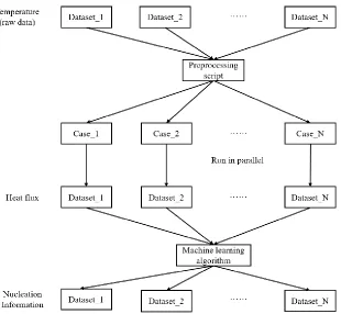
17 CHAPTER 3. DATA PROCESSING AND STORAGE
This chapter discusses the data processing and storage procedure of the data-driven analysis framework. The nucleate boiling is a complex multiphysics process that involves interactions between heating surface, liquid, and vapor. Thus the data related to boiling also have complex structures. Moreover, different applications could be developed based on one dataset, whereas one application could also depend on several interrelated datasets. To maximize the convenience of data usage, the concept of “virtual container” is adopted for the storage of the obtained data.
In this chapter, the data processing procedure is applied to both high-resolution experiments and high-fidelity simulations. Multiple QoIs are extracted and stored in the virtual container. The purpose of this procedure is to convert the heterogeneous rich data to well organized datasets that can be conveniently used for quantifying or reducing the uncertainty of MCFD solver through various applications.
3.1 Processing boiling images from IR camera
The data measured by high-speed infrared (IR) camera in both pool boiling and subcooled flow boiling experiments are studied in this work. A typical IR experiment is demonstrated in Figure 3. These experiments used nano-meter-thick metal film deposited on a glass substrate for ohmic heating. This design ensures uniform heat flux distribution on heating surface. The transparency of glass ensures it is the heating surface’s infrared that is captured by the camera. For subcooled flow boiling, the setup is similar with a different direction. The data from both the pool boiling experiments (UCSB-BETA) [25, 26] and subcooled flow boiling experiments (from MIT boiling experimental facility) [45] are processed in this work.
18 equation over the substrate is solved to obtain the heat flux distribution over the heating surface. With the heat flux obtained, the nucleation information including the location of active nucleation sites, the heat partitioning, the bubble area fraction, etc. can be obtained. This is done through a parallel processing system as depicted in Figure 4. The detailed work would be discussed in Section 3.1.2.
Figure 3. Schematic of measuring high-resolution boiling process with IR camera.
19 3.1.1 Heat flux distribution processing
For UCSB-BETA experiment, the heat flux is obtained by solving transient three-dimensional heat conduction equation for the glass substrate, as shown in Figure 5. A special type of boundary condition is developed to map the IR temperature data to the upper wall cells. The surrounding walls are assumed to be adiabatic, while the lower wall is assumed to be a mixed boundary type with constant heat transfer coefficient. Grid sensitivity is conducted to ensure the obtained results are mesh independent.
Figure 5. Scheme of computational domain for deriving heat flux distribution on heating surface.
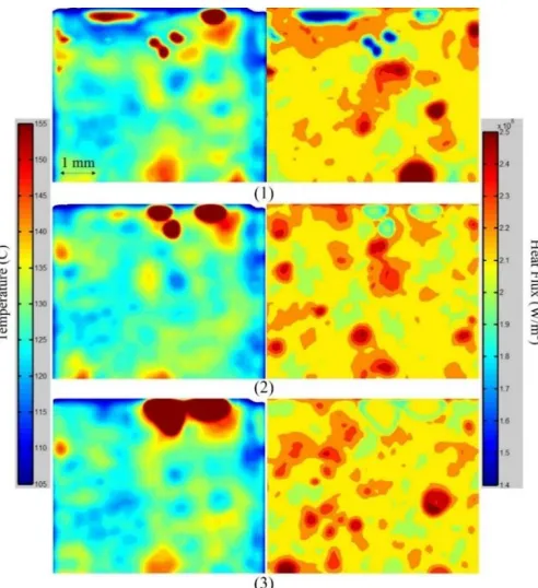
20 An example of obtained results are demonstrated in Figure 6. The development of the boiling crisis can be directly observed from these images.
Similar process is performed for the subcooled flow boiling experiments. Figure 7 demonstrates an example of the obtained temperature and heat flux distribution. As can be seen, the sliding effect can be clearly observed in the heat flux map.
Figure 7. Temperature and corresponding heat flux distribution in flow boiling, mass flow rate = 500kg/m2, heat flux = 1.4MW/m2.
3.1.2 Nucleation information processing
21 learning algorithm is applied to automatically identify and record the nucleation information.
The hierarchical clustering algorithm is applied to the obtained heat flux images to identify the active nucleation sites. There are two types of hierarchical clustering, the agglomerative and divisive. In this work, the agglomerative type is adopted, which is a “bottom up” approach. Each sample starts in its own cluster, in each iteration, pairs of clusters are merged until the stop criterion is satisfied.
The clustering process is dependent on measuring the dissimilarity, which is usually represented by distance, between sets of samples. Such measurement is specified by a chosen metric and the corresponding linkage criterion. The metric determines how to measure the dissimilarity, while the linkage criterion determines based on which property of the cluster to measure the dissimilarity. The commonly used metrics for hieratical clustering includes: Euclidean distance, Maximum distance, Mahalanobis distance, etc.
In this work, the Euclidean distance is chosen as the metric,
‖𝒂 − 𝒃‖2 = √∑(𝑎𝑖 − 𝑏𝑖)2 𝑖
, (1)
where 𝑖 is the dimension of the sample. In this work, the clustering is applied to pixels of an image, thus 𝑖 = 2.
A cluster consists of multiple samples; thus the metric alone cannot generate a unique distance between two clusters. The linkage criterion is introduced to resolve this issue and provide a unique measurement for the distance between two clusters. The maximum linkage criterion, for example, defines the distance between two clusters 𝐴 and 𝐵 as the maximum pairwise distance of samples inside 𝐴 and 𝐵. The minimum linkage criterion, in contrast, defines the distance as the minimum pairwise distance of samples inside 𝐴 and 𝐵. In this work, the centroid linkage is chosen, which means the Euclidean distance between two clusters 𝐴 and 𝐵 is calculated by
22 where 𝑐𝐴 and 𝑐𝐵 are the centroids of clusters 𝐴 and 𝐵, respectively.
Before running the clustering process, a value is specified to the linkage criterion, the merging process will stop when the distance between every pair of clusters exceed this value. This value needs to be adjusted for each case, since a too large value would falsely merge two nucleation sites into one, while a too small value would falsely divide one nucleation sites into several. In the practice, around 50 frames are randomly chosen from each case to manually examine if the clustering is correct or not, based on which the linkage value is adjusted.
Figure 8. Example of hierarchical clustering for active nucleation sites identification. An example of the hierarchical clustering for active nucleation sites identification is demonstrated in Figure 8, it can be found that even the very small incipient nucleation sites can be identified.
23 Figure 9. Evaporation Heat Flux and Bubble Area Fraction Distributions, 𝑞 =
1.16 MW/m2, BETA experiment, Heater Ti36A.
These obtained boiling data can serve multiple purpose. First, it provides direct observation to the detailed boiling process that provide better understanding of the flow boiling process and the boiling crisis. This could serve a foundation for new mechanistic closure relation development. Second, the obtained data can be further averaged over time and space to serve for the VUQ of wall boiling closure relation in MCFD solver. Last, coupling with the flow dynamics measurement, the data can be used for data-driven modeling. In this dissertation, only the second application is developed, but it should be noted that more applications can be development with these high-resolution data.
3.2 Processing high-fidelity simulation results
The high-fidelity simulation results are processed to serve for data-driven modeling purpose, as will be discussed in Chapter.5. The simulation studied multiple pool boiling scenarios with interface tracking method (ITM) [46]. The simulation is based on directly solving the incompressible Navier-Stokes equations with a sharp-interface, phase-change model proposed in [30]. The three conservative equations solved in this approach can be expressed as follows:
Mass:
𝜕𝜌
𝜕𝑡 + ∇ ∙ 𝜌𝑼 = 0 , (3)
24 𝜕𝜌𝑼
𝜕𝑡 + ∇ ∙ (𝜌𝑼𝑼) = −∇𝑝 + ∇ ∙ {𝜇(∇𝑼 + (∇𝑼)
𝑻)} + 𝒇 , (4) Energy:
C𝑝(𝜕𝑇
𝜕𝑡 + 𝑼 ∙ ∇𝑇) = ∇ ∙ (𝜆∇𝑇) + 𝑄 , (5)
In addition to the conservative equations, the color function 𝜙 is used to track the interface between vapor and liquid:
𝜕𝜙
𝜕𝑡 + ∇ ∙ (𝜙𝑼) = − 1
𝜌𝒍𝛤𝒍𝒗 , (6)
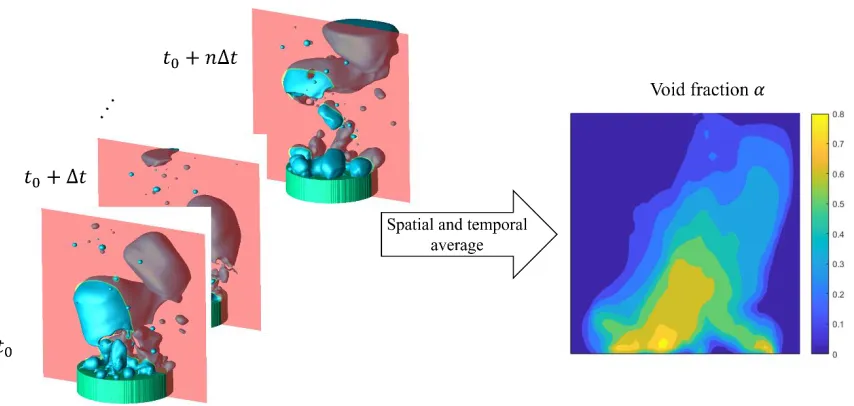
In the simulation, the nucleation site is prescribed in the whole heating surface, and the heat conduction in the solid wall is considered through conjugate heat transfer. With the boundary conditions specified, the solver is able to predict the detailed boiling process with high accuracy. The QoIs of boiling process include the wall superheat, evaporation heat transfer component, convective heat transfer component towards liquid, and near wall bubble concentration. Such QoIs are the outcome of complex interactions between different phenomena, including: convection, evaporation, conjugate heat transfer, buoyancy, and nucleation. Although it is impossible to develop an explicit correlation or a model to accurately account for such interaction and give a reasonable prediction for the QoIs, a DNN that takes those phenomena as input features can serve as a “black-box” model for the prediction of boiling QoIs and can be applied to untested conditions.
On the other hand, however, the ITM simulation is performed on very fine meshes, the results contain detailed interface information, as well as the fluctuation of physical quantities. For the two-fluid-model, such information is unnecessary. In this sense, the obtained ITM results need to go through certain average process before being used for training the DNN which is supposed to be compatible with two-fluid-model.
In this work, a combination of time and space average is processed for each physical quantities 𝑓(𝒙, 𝑡) into a space and time averaged form 〈𝑓〉(𝒙, 𝑡) which can be described as follows:
〈𝑓〉(𝒙, 𝑡) =1 𝜏
1
𝑙3∫ ∫ ∫ ∫ 𝑓(𝒙′, 𝑡′)𝑑𝑥3′𝑑𝑥2′𝑑𝑥1′𝑑𝑡′ 𝑥3+𝑙/2
𝑥3−𝑙/2 𝑥2+𝑙/2
𝑥2−𝑙/2 𝑥1+𝑙/2
𝑥1−𝑙/2
, 𝑡
𝑡−𝜏
25 where 𝜏 and 𝑙 are the averaging time scale and averaging length scale, respectively. One interesting fact that worth noting ,as discussed in [47], is that this average process is mathematically equivalent to the convolution operation over a 4-dimensional matrix (three dimension in space, one dimension in time), with a kernel function𝑔(𝒙):
〈𝑓〉(𝒙, 𝑡) = ∫ ∫ ∫ ∫ 𝑔(𝒙 − 𝒙′) 𝑅4
𝑓(𝒙′, 𝑡)𝑑𝒙′ . (8)
For quantities that are only valid in the heating surface, i.e. the potential nucleation site density, nucleation activation temperature, wall superheat, and the heat transfer components, the average process is performed on 2-dimensional surface and time. Such operation is widely adapted in the DNN for extracting and preserving features of the data. It is assumed the averaged process will preserve the causal-relationship between input features and the boiling QoIs. Such assumption is reasonable if the ITM simulation already reached quasi-steady state before the data is extracted. Every physical quantity obtained from the ITM simulation are propagated through the process to generate an averaged version of it. The void fraction 𝛼 is obtained by propagating color function 𝜙 through this process. One example of the average process is demonstrated in Figure 10, where the color function describing the bubble interface is averaged over time and space to generate the void fraction distribution over a slice plane.
26 After this average process, the raw data of hundreds gigabyte level would be reduced to hundreds megabyte level while still preserves all the important information.
3.3 “Virtual container” for data storage
The processed data should be properly stored for the future usage. There are different purposes to use these datasets, one researcher hope to investigate the relevant physical process from the data, another researcher wants to use the data to validate a model, while another researcher would like to develop a new model based on the data. In this sense, the data need to be stored in a flexible way to maximize the convenience for all purposes. Moreover, potential connections could exist between different datasets, thus the data storage should also be flexible to preserve such possible connection. Based on this, the concept of “virtual container” proposed in the Nuclear Energy Knowledgebase for Advanced Modeling and Simulation (NE-KAMS) [48] is adopted in this dissertation.
With this concept, datasets are stored in virtual containers according to the facility and the experimental condition. That is, no matter how many measurements was taken in one experiment, how many QoIs are measured and what their types are, it should be stored together in one container. This container should have a clear description about the information it stored and should provide access to all types of data it stored so other researchers that is not familiar with this experiment can still understand and use them. An example of virtual container storing the subcooled flow boiling data is given in Table 1. In this dissertation, the virtual container is stored in the dataframe format supported by Pandas, which is a python package.
27 Table 1. Example of an experimental data container
General information
Source MIT boiling experimental facility [45] System configuration
Geometry Vertical flow in rectangular channel
Fluid materials water liquid/vapor Heater materials ITO sapphire heater with
synthetic CRUD Test program
Flow conditions 500 kg/m2
Heat configurations
2um thick CRUD with 10um diameter chimneys
on a 45um pitch
Heat flux 1400 kW/m2
Data stored
[D0] raw data IR counts distribution [D1] data type I temperature/heat flux
distribution [D2] data type II Nucleation information
[D3] data type III
Averaged heater temperature and heat
transfer partition Data characteristics
Applicability
boiling model VUQ for flow boiling on low
pressure
28 Figure 11. Collaboration between two virtual containers.
3.4 Summary remarks
In this chapter, the data processing and storage procedure is introduced with two examples. The purpose of this procedure is to convert the heterogeneous rich data to well organized datasets that can be conveniently used for quantifying or reducing the uncertainty of MCFD solver through various applications.
The hierarchical clustering algorithm is applied for the high-resolution IR boiling experiments. Active nucleation sites and the corresponding nucleation information can be automatically identified with the algorithm. Boiling related QoIs for MCFD solver are extracted. Similarly, the time and space average process is applied to high-fidelity ITM simulations. The extracted data are organized in the virtual container for further usage.
29 CHAPTER 4. METHODOLOGY DEVELOPMENT FOR THE VALIDATION
AND UNCERTAINTY QUANTIFICATION FOR MCFD SOLVER
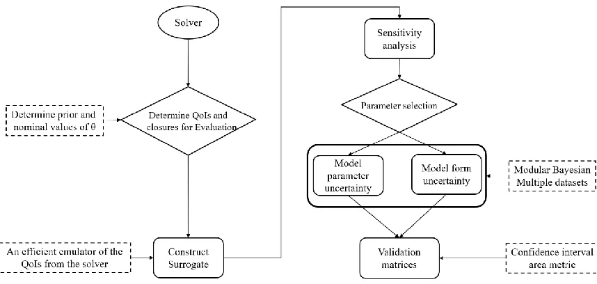
In this chapter, a validation and uncertainty quantification (VUQ) procedure for the Eulerian-Eulerian two-fluid-model based multiphase-computational fluid dynamics solver (MCFD) is developed. The procedure aims to answer the question: how to evaluate if a MCFD solver adequately represents the underlying physics of a multiphase system of interest? The proposed procedure is based on total data-model integration (TDMI) approach that uses Bayesian method to inversely quantify the uncertainty of the solver predictions with the support of multiple experimental datasets. The framework consists of six steps with state-of-the-art statistical methods, including: 1). Solver evaluation and data collection; 2). Surrogate model construction; 3). Sensitivity Analysis; 4). Parameter selection; 5). Uncertainty quantification with Bayesian inference; and 6). Validation metrics calculation. Those steps are formulated in a modular manner and using non-intrusive methods. Such features ensure the applicability of the flexible procedure to different scenarios and modeling of multiphase flow and boiling heat transfer, as well as the extensibility of the procedure to support VUQ of different MCFD solvers.
4.1 Eulerian-Eulerian two-fluid model based MCFD solver
The fundamental idea of a two-fluid-model is to average the local instantaneous conservation equations, thus eliminating the need for tracking interfaces to achieve computational efficiency. The system of averaged conservation equations needs to be solved numerically, commonly using a finite-volume or finite-element method. The convergence and accuracy of the solution depend on numerical techniques and temporal and spatial resolutions needed to capture the dynamics and scales of governing physical processes.
4.1.1 Conservative equations
30 ∂(𝛼𝑘𝜌𝑘)
∂𝑡 + ∇ ⋅ (𝛼𝑘𝜌𝑘𝐔𝑘) = 𝛤𝑘𝑖− 𝛤𝑖𝑘 , (9) where the two terms on the left-hand side represent the rate of change and convection, the two terms on the right-hand side represent the rate of mass exchanges between phases due to condensation and evaporation.
The k-phasic momentum equation is given by ∂(𝛼𝑘𝜌𝑘𝐔𝑘)
∂𝑡 + ∇ ⋅ (𝛼𝑘𝜌𝑘𝐔𝑘𝐔𝑘) = −𝛼𝑘∇𝑝𝑘+ ∇ ⋅ [𝛼𝑘(𝜏𝑘+ 𝜏𝑘 𝑡)] + 𝛼
𝑘𝜌𝑘𝐠 + 𝛤𝑘𝑖𝐔𝑖 − 𝛤𝑘𝑖𝐔𝑘+ 𝐌𝑘𝑖,
(10) where i represents the interphase between two phases, 𝐌𝑘𝑖 represents the term of averaged interfacial momentum exchange, which can be modeled by a set of interfacial force closure relations.
The k-phasic energy conservation equation in terms of specific enthalpy can be given as
∂(𝛼𝑘𝜌𝑘ℎ𝑘)
∂𝑡 + ∇ ⋅ (𝛼𝑘𝜌𝑘ℎ𝑘𝐔𝑘) = ∇ ⋅ [𝛼𝑘(𝜆𝑘𝛻𝑇𝑘− 𝜇𝑘
Pr𝑘𝑡 𝛻ℎ𝑘)] + 𝛼𝑘 𝐷𝑝
𝐷𝑡+ 𝛤𝑘𝑖ℎ𝑖 − 𝛤𝑖𝑘ℎ𝑘+ 𝑞𝑘 ,
(11)
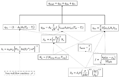
where the terms on the right-hand side represent heat transfer in phase k, work done by pressure, enthalpy change due to evaporation and condensation, and heat flux from the wall. The wall boiling heat transfer is modeled by a set of closure relations.
4.1.2 Characterization of closure relations in MCFD
31 for the interphase exchange of mass, momentum and energy. Interfacial force closure relations are proposed to describe the interphase momentum exchange, while interfacial condensation closure is necessary to describe the interphase mass and heat transfer for the subcooled flow boiling problem. Moreover, the size of bubbles has significant influence on those interphase exchanges, and closure relation is needed for determining the bubble size. Last, the turbulence can influence the interphase exchange, and the bubble dynamics in turn influences the turbulence, thus closure relation is also required to describe the bubble-induced turbulence. Thus the closure relations in a MCFD solver can be characterized into five categories: wall boiling, interfacial momentum exchange, interfacial mass/heat transfer, bubble size, and turbulence. There exist complex relationships between those closure relations and a typical structure of them is depicted in Figure 12.
32 Figure 12. Closure relation structures in a typical MCFD solver.
Turbulence
33 flow -is modeled in this way, while the turbulent viscosity of dispersed phase is assumed to be linearly dependent on the vt of continuous phase with a turbulence response
coefficient Ct.
Interfacial momentum closure relations
The interfacial momentum exchange between two phases is represented by different types of interfacial forces. For a typical MCFD solver, five interfacial forces are modeled. The drag force is modeled to describe the resistance of relative motion between the two phases. The lift force is modeled to describe the force that exerts by continuous fluid flow past the bubble. The turbulent dispersion force is modeled to describe the effect of liquid turbulence on the bubble. The wall lubrication force is designed as an artificial force to move the bubble away from the wall to describe. The virtual mass force is modeled to describe the inertia of bubble acceleration or deceleration. Figure 13 illustrates these five interfacial forces.
Figure 13. Schemes of interfacial forces.
Table 2 summarizes the expressions of those interfacial forces. Among these interfacial forces, the form of drag force and lift force can be analytically derived; thus their expression is quite consistent among different MCFD solvers. On the other hand, the force coefficients Cdand Cl are calculated from semi-empirical correlations. For drag force,
34 practices, the force coefficients are also set to be constant for simplification purpose. The forms of other three forces is varied among different researchers due to the lack of solid theoretical support. Besides the expressions summarized in Table 2, there are other expressions can be used, such as the wall lubrication force model proposed by [53] turbulent dispersion force model proposed by [54].
Table 2. Expressions of interfacial forces
Force type Expression
Drag force 𝐌𝑔𝐷 = −3
4 𝐶𝑑
𝐷𝑠𝜌𝑙𝛼‖𝐔𝑔− 𝐔𝑙‖(𝐔𝑔 − 𝐔𝑙)
Lift force 𝐌𝑔𝐿 = 𝐶𝑙𝜌𝑙𝛼(𝐔𝑔− 𝐔𝑙) × (∇ × 𝐔𝑔)
Wall lubrication force [55]
𝐌𝑔𝑊𝐿 = −𝑓𝑊𝐿(𝐶𝑤𝑙, 𝑦𝑤)𝛼𝜌𝑙
‖𝐔𝑟− (𝐔𝑟⋅ 𝐧𝑤)𝐧𝑤‖2 𝐷𝑠
𝐧𝑤 ,
𝑓𝑊𝐿(𝐶𝑤𝑙, 𝑦𝑤) = max (−0.2𝐶𝑤𝑙+ (𝐶𝑤𝑙
𝑦𝑤)𝐷𝑠, 0)
Turbulent dispersion force
[56] 𝐌𝑔
𝑇𝐷 = −3 4 𝐶𝐷 𝐷𝑠 𝜐𝑙𝑡 𝜎𝑡𝑃𝑟 𝑙𝑡 𝜌𝑙‖𝐔𝑔− 𝐔𝑙‖∇𝛼
Virtual mass force
[57] 𝐌𝑔
𝑉𝑀= −𝐶 𝑣𝑚𝜌𝑙𝛼 ( 𝐷𝐔𝑔 𝐷𝑡 − 𝐷𝐔𝑙 𝐷𝑡)
Interfacial mass and heat transfer closure relations
Bubbles developed from nucleation depart from the wall and join the bulk flow. In subcooled flow boiling, the bubbles become surrounded by the subcooled liquid causing vapor condensation. The interfacial mass transfer related to condensation of vapor bubbles in the bulk coolant can be described as
𝛤lg = ℎ𝑙𝑔(𝑇𝑠𝑎𝑡− 𝑇𝑙)𝐴𝑎
ℎ𝑓𝑔 , (12)
35 Bubble size closure relations
The size of the bubble has significant influence on the interphase exchanges of mass, energy, and momentum. Initially, the bubble size is evaluated using empirical correlation derived from subcooled flow boiling. One example of the empirical correlation, as proposed by [60], is
𝐷𝑠 = 𝐷𝑟𝑒𝑓,1(𝑇𝑠𝑢𝑏− 𝑇𝑠𝑢𝑏,2) + 𝐷𝑟𝑒𝑓,2(𝑇𝑠𝑢𝑏,1− 𝑇𝑠𝑢𝑏)
𝑇𝑠𝑢𝑏,1− 𝑇𝑠𝑢𝑏,2 , (13)
where 𝑇𝑠𝑢𝑏,1, 𝑇𝑠𝑢𝑏,2, 𝐷𝑟𝑒𝑓,1, 𝐷𝑟𝑒𝑓,2 are empirical constants which have suggested values, but those values are often tuned in different applications. A more sophisticated development is to predict the bubble size distribution with the interfacial area transport equation [61]. The volumetric interfacial area concentration equation can be expressed as
∂(𝐴𝑎)
∂𝑡 + ∇ ⋅ (𝐴𝑎𝐔𝑎) = 2 3
𝐴𝑎 𝛼 (
𝜕𝛼
𝜕𝑡 + 𝛻 ⋅ (𝛼𝐔𝑎)) + ΦBB+ ΦBC+ ΦNUC , (14) in which the first term on the right-hand side refers to the contribution of phase change and expansion due to pressure-density change. Here ΦBB, ΦBC, and ΦNUC represent the source and sink term induced by breakup, coalescence, and nucleation respectively. There are several semi-empirical correlations for those terms proposed by different researchers, reprehensive works include [62], and [63].
Another mechanistic approach for bubble size prediction is the multiple size group (MUSIG) model which deals with the non-uniform bubble size distribution by dividing the bubble size distribution into a finite number of groups. A more recent progress is the inhomogeneous MUSIG model by [64] which allows each bubble group to have its own velocity.
Wall boiling closure relations