ABSTRACT
FISHER, CHRISTOPHER BRANT. Deterministic Modeling and Analysis of U.S. Army Recruiting Policies and Resulting Force Composition. (Under the direction of Thom Hodgson.)
Specialized U.S. Army units need to take many factors into account when establishing their recruiting goals. These units may recruit from both Active Duty (AD) and Non-Prior Service (NPS) populations, each of which brings different strengths to the unit. For this reason, the unit may desire to maintain a specific ratio of assigned AD and NPS personnel at any given time. Additionally, these populations successfully complete required training at different rates, and are also retained at different rates after joining the unit. Since today’s recruiting goals will impact the unit for 20 years or more, units need to take all of these factors into account from a long-term perpsective when establishing their recruiting goals. Units also need to assign recruits their Military Occupational Specialties (MOS) in a way that fills the unit’s authorizations as close to 100% as possible.
This paper aims to model the problem and create a tool that can be used by a specific U.S. Army unit to analyze their force composition over time as a function of recruiting policies and methods of MOS assignment. A deterministic model was constructed representing the processes of new recruits completing pre-requisites and going through training, and the assigned force changing over time, using historical training and continuation rates. This model was used to build an analysis tool the unit can use to assist with establishing recruiting goals each year. The tool provides the unit with the ability to easily test what the projected long-term results of their proposed recruiting policies are. The tool also gives them the ability to see how changes in policy to effect changes to current rates can be used to make improvements to the results of a recruiting policy.
© Copyright 2016 by Christopher Brant Fisher
Deterministic Modeling and Analysis of U.S. Army Recruiting Policies and Resulting Force Composition
by
Christopher Brant Fisher
A thesis submitted to the Graduate Faculty of North Carolina State University
in partial fulfillment of the requirements for the Degree of
Master of Science
Operations Research
Raleigh, North Carolina
2016
APPROVED BY:
Robert Young Michael Kay
Thom Hodgson
DEDICATION
Dedicated to my wife Lindsay.
BIOGRAPHY
Chris Fisher was born, raised, and home schooled in Illinois before attending college at Cedarville Univeristy in Ohio, where he received a B.S. in Mathematics in 2007. He participated in the Central State University ROTC program and received a commission as a Second Lieutenant in the United States Army. In the Army he has served as both an Infantry and Adjutant General Officer, completing assignments as a Platoon Leader, Company Executive Officer, and Cavlary Squadron Human Resource Officer from 2008 to 2014, including two deployments to Afghanistan in support of Operation Enduring Freedom. In the summer of 2014 he moved to Raleigh, North Carolina to study Operations Research at North Carolina State Univeristy, upon completion of which he will be assigned to the Mathematics Department of the United States Military Academy at West Point, NY.
ACKNOWLEDGEMENTS
First, thanks to God who has blessed me greatly with the chance to do this work. Special thanks to my committee members, Dr. Hodgson, Dr. Kay, and Dr. Young for their support in conducting research in an area which I am very passionate about and giving me the tools to succeed. Also, thank you to the U.S. Army for providing the opportunity to further my education.
TABLE OF CONTENTS
LIST OF TABLES . . . .viii
LIST OF FIGURES . . . x
Chapter 1 Introduction . . . 1
1.1 Background . . . 1
1.1.1 U.S. Army Structure and Organization . . . 1
1.1.2 US Army Enlisted Recruiting . . . 2
1.1.3 US Army Enlisted Training . . . 3
1.2 The Problem . . . 3
1.2.1 Unit Organization and Manning Goals . . . 3
1.2.2 Decision Points and Current Methods . . . 4
1.2.3 Purpose . . . 6
1.3 Thesis Structure . . . 6
Chapter 2 Data Formulation . . . 7
2.1 Data Used . . . 7
2.1.1 Data Sources . . . 7
2.1.2 Data Organization . . . 7
2.2 Data Preparation . . . 11
2.2.1 Data Cleansing . . . 11
2.2.2 Converting to Model Input . . . 12
2.2.3 Additional Model Inputs/Assumptions . . . 15
Chapter 3 Modeling . . . 17
3.1 Model Development and Basic Reports . . . 17
3.1.1 Initial Approach . . . 17
3.1.2 Report 1: Single MOS Report . . . 18
3.1.3 Report 2: Multiple MOS Report . . . 21
3.1.4 Report 3: Training Report . . . 23
3.2 Report 4: Force Projection Report . . . 28
3.2.1 Report Development . . . 28
3.2.2 Report Layout and Output . . . 35
3.3 Validation . . . 40
3.3.1 Method . . . 40
3.3.2 Changes Made to Data . . . 40
3.3.3 Results . . . 41
Chapter 4 Analysis and Recommendations . . . 44
4.1 Analysis Approach . . . 44
4.2 Policy 1 . . . 45
4.2.1 Base Case . . . 45
4.2.2 Changes Made . . . 46
4.2.3 Recommendation . . . 50
4.3 Policy 2 . . . 50
4.3.1 Base Case . . . 50
4.3.2 Changes Made . . . 50
4.3.3 Recommendation . . . 55
4.4 Policy 3 . . . 55
4.4.1 Base Case . . . 55
4.4.2 Changes Made . . . 55
4.4.3 Recommendation . . . 56
4.5 Policy 4 . . . 60
4.5.1 Base Case . . . 60
4.5.2 Changes Made . . . 60
4.5.3 Recommendation . . . 61
Chapter 5 Conclusion . . . 65
5.1 Summary . . . 65
5.2 Future Work . . . 67
References. . . 68
APPENDICES . . . 69
Appendix A Model Input . . . 70
A.1 PRM Data . . . 70
A.2 Training Data . . . 79
Appendix B Model . . . 84
B.1 User Instructions . . . 84
B.1.1 Updating Personnel Readiness Management Data . . . 84
B.1.2 Updating Training Rates, Training Delay, and Course Information . 85 B.1.3 Graduate Based Force Composition Projection for a Single MOS . . 85
B.1.4 Graduate Based Force Composition Projection for All MOS’s . . . . 86
B.1.5 Recruit Based Graduate Projection . . . 86
B.1.6 Recruit Based Force Composition Projection . . . 87
B.2 Forms . . . 89
B.2.1 AttritionComp frm . . . 89
B.2.2 ComparisonOpt frm . . . 97
B.2.3 CourseComp frm . . . 102
B.2.4 CRComp frm . . . 113
B.2.5 Main frm . . . 121
B.2.6 MOSCRComp frm . . . 123
B.2.7 MOSDistOpt frm . . . 134
B.2.8 MOSDistSel frm . . . 137
B.2.9 MOSGradSel frm . . . 144
B.2.10 PrintOptions frm . . . 151
B.2.11 PRM frm . . . 164
B.2.12 RecruitGoal frm . . . 173
B.2.13 Report1 frm . . . 178
B.2.14 Report2 frm . . . 185
B.2.15 Report3 frm . . . 214
B.2.16 Report4 frm . . . 241
B.2.17 Report5Input frm . . . 261
B.2.18 Reports frm . . . 297
B.2.19 Training frm . . . 304
B.3 Print Report . . . 319
B.3.1 Purpose . . . 319
B.3.2 Subreport Names, Sources, Controls, and VBA Code . . . 319
B.4 VBA Public Module . . . 324
Appendix C Glossary of Military Acronyms . . . 377
LIST OF TABLES
Table 2.1 Attrition Events with Pass Rates by Graduate Type . . . 8
Table 2.2 Course C4 Class 14-001 Data . . . 8
Table 2.3 Sample of Assigned Data Format . . . 9
Table 2.4 Sample of CR and MOS Change Data: FY 2012 M1/AD Data . . . 10
Table 3.1 Projected number of graduates per year by recruit year . . . 31
Table 3.2 AD and NPS Overall Course Pass Rates for FY12 - FY15 . . . 41
Table 3.3 Actual vs. projected number assigned on October 1st, 2015 . . . 42
Table 3.4 Actual vs. Projected MOS fill as a percent of total assigned on October 1st, 2015 . . . 42
Table 4.1 Number of annual recruits for each policy; annual PSA gains remain constant at 25 for all policies. . . 45
Table A.1 PRMtbl . . . 70
Table A.2 TrainingRatestbl . . . 79
Table A.3 TrainingDelaytbl . . . 82
Table B.1 Form AttritionComp frm Controls . . . 91
Table B.2 Form AttritionComp frm Associated Queries . . . 91
Table B.3 Form ComparisonOpt frm Controls . . . 98
Table B.4 Form CourseComp frm Controls . . . 104
Table B.5 Form CourseComp frm Associated Queries . . . 104
Table B.6 Form CRComp frm Controls . . . 115
Table B.7 Form CRComp frm Associated Queries . . . 115
Table B.8 Form Main frm Controls . . . 122
Table B.9 Form MOSCRComp frm Controls . . . 126
Table B.10 Form MOSCRComp frm Associated Queries . . . 126
Table B.11 Form MOSDistOpt frm Controls . . . 135
Table B.12 Form MOSDistSel frm Controls . . . 138
Table B.13 Form MOSDistSel frm Associated Queries . . . 138
Table B.14 Form MOSGradSel frm Controls . . . 146
Table B.15 Form MOSGradSel frm Associated Queries . . . 146
Table B.16 Form PrintOptions frm Controls . . . 152
Table B.17 Table PRM tbl Required Structure for Importing from Excel . . . 165
Table B.18 Form PRM frm Controls . . . 167
Table B.19 Form PRM frm Associated Queries . . . 167
Table B.20 Form RecruitGoal frm Controls . . . 174
Table B.21 Form Report1 frm Controls . . . 180
Table B.22 Form Report1 frm Associated Queries . . . 180
Table B.23 Form Report2 frm Controls . . . 188
Table B.24 Form Report2 frm Associated Queries . . . 189
Table B.25 Form Report3 frm Controls . . . 216
Table B.26 Form Report3 frm Associated Queries . . . 216
Table B.27 Form Report4 frm Controls . . . 244
Table B.28 Form Report4 frm Associated Queries . . . 244
Table B.29 Form Report5Input frm Controls . . . 264
Table B.30 Form Report5Input frm Associated Queries . . . 265
Table B.31 Form Reports frm Controls . . . 298
Table B.32 Table TrainingDelay tbl Required Structure for Importing from Excel . . . . 305
Table B.33 Table TrainingRates tbl Required Structure for Importing from Excel . . . . 305
Table B.34 Form Training frm Controls . . . 307
Table B.35 Form Training frm Associated Queries . . . 307
Table B.36 Subreport Names and Sources . . . 319
Table B.37 Report Summary rpt Controls and Sources . . . 320
Table C.1 Military Acronyms Used . . . 377
LIST OF FIGURES
Figure 1.1 New Recruit Path to Unit . . . 4
Figure 1.2 MOS Interactions Within Unit . . . 5
Figure 3.1 Report 1: Projected YOS distribution and total assigned for M1/AD at the end of 20 years, given 150 annual graduates and 10 annual PSA gains . . . . 19
Figure 3.2 Report 1 Model Process . . . 20
Figure 3.3 Report 2: Projected force composition based on a user provided number of annual graduates of each MOS and GT. . . 22
Figure 3.4 Report 3: Projected graduates and availability for 1000 AD and 1000 NPS recruits using authorizations-based MOS distribution . . . 24
Figure 3.5 Current Shortages Method Algorithm . . . 26
Figure 3.6 Report 4 logical flow; steps 3-5 are repeated for each year of the projection. 29 Figure 3.7 Report 4 continuation rate comparison options form . . . 31
Figure 3.8 Report 4 MOS change rate comparison options form . . . 32
Figure 3.9 Report 4 training course comparison options form . . . 33
Figure 3.10 Report 4 attrition comparison options form . . . 34
Figure 3.11 Report 4: Comparison Form . . . 36
Figure 3.12 Report 4: Single Option Details Form . . . 37
Figure 3.13 Report 4 Results Report Sub-Report Options . . . 38
Figure 3.14 Report 4 Results Report: Report Summary Sub-report . . . 39
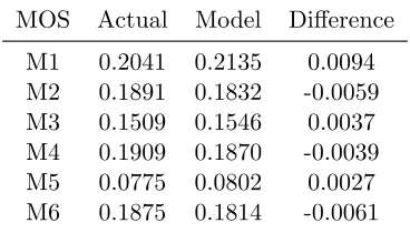
Figure 4.1 Policy 1 Base Case Results . . . 47
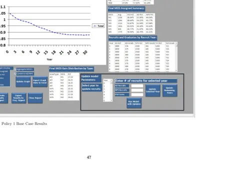
Figure 4.2 Policy 1a, 1b, and 1c Results . . . 48
Figure 4.3 Policy 1 Final Recommendation Detailed Results . . . 49
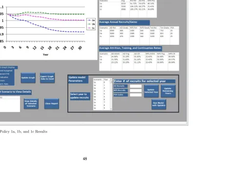
Figure 4.4 Policy 2 Base Case Results . . . 52
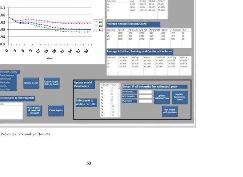
Figure 4.5 Policy 2a, 2b, and 2c Results . . . 53
Figure 4.6 Policy 2 Final Recommendation Detailed Results . . . 54
Figure 4.7 Policy 3 Base Case Results . . . 57
Figure 4.8 Policy 3a, 3b, and 3c Results . . . 58
Figure 4.9 Policy 3 Final Recommendation Detailed Results . . . 59
Figure 4.10 Policy 4 Base Case Results . . . 62
Figure 4.11 Policy 4a, 4b, and 4c Results . . . 63
Figure 4.12 Policy 4 Final Recommendation Detailed Results . . . 64
Figure B.1 Form AttitionComp frm . . . 90
Figure B.2 Form AttritionComp frm VBA Code . . . 92
Figure B.3 Form ComparisonOpt frm . . . 98
Figure B.4 Form ComparisonOpt frm VBA Code . . . 99
Figure B.5 Form CourseComp frm . . . 103
Figure B.6 Form CourseComp frm VBA Code . . . 105
Figure B.7 Form CRComp frm . . . 114
Figure B.8 Form CRComp frm VBA Code . . . 116
Figure B.9 Form Main frm . . . 122
Figure B.10 Form Main frm VBA Code . . . 123
Figure B.11 Form MOSCRComp frm . . . 125
Figure B.12 Form MOSCRComp frm VBA Code . . . 127
Figure B.13 Form MOSDistOpt frm . . . 135
Figure B.14 Form MOSDistOpt frm VBA Code . . . 136
Figure B.15 Form MOSDistSel frm . . . 138
Figure B.16 Form MOSDistSel frm VBA Code . . . 139
Figure B.17 Form MOSGradSel frm . . . 145
Figure B.18 Form MOSGradSel frm VBA Code . . . 147
Figure B.19 Form PrintOptions frm . . . 151
Figure B.20 Form PrintOptions frm VBA Code . . . 153
Figure B.21 Form PRM frm . . . 166
Figure B.22 Form PRM frm VBA Code . . . 168
Figure B.23 Form RecruitGoal frm . . . 174
Figure B.24 Form RecruitGoal frm VBA Code . . . 175
Figure B.25 Form Report1 frm . . . 179
Figure B.26 Form Report1 frm VBA Code . . . 181
Figure B.27 Form Report2 frm . . . 187
Figure B.28 Form Report2 frm VBA Code . . . 190
Figure B.29 Form Report3 frm . . . 215
Figure B.30 Form Report3 frm VBA Code . . . 217
Figure B.31 Form Report4 frm . . . 243
Figure B.32 Form Report4 frm VBA Code . . . 248
Figure B.33 Form Report5Input frm . . . 263
Figure B.34 Form Report5Input frm VBA Code . . . 266
Figure B.35 Form Reports frm . . . 297
Figure B.36 Form Reports frm VBA Code . . . 299
Figure B.37 Form Training frm . . . 306
Figure B.38 Form Training frm VBA Code . . . 308
Figure B.39 Report Print rpt VBA Code . . . 321
Figure B.40 Public Module VBA Code . . . 325
Chapter 1
Introduction
1.1
Background
1.1.1 U.S. Army Structure and Organization
In order to understand the problem at hand, some general knowledge of US Army organizational structure is necessary. The US Army is broadly broken down into two categories of personnel: Officers (both Commissioned Officers and Warrant Officers) and Enlisted Members. Each category has its own requirements, training, and mission set (AR 600-20). This paper focuses on Enlisted Members, and henceforth all references to “Soldiers” refer exclusively to Enlisted Soldiers.
The Army is made up of different nested organizations known as units (DA PAM 10-1). Different units have different functions, and are not generally interchangeable. An Infantry Brigade Combat Team, for example, cannot achieve the same results as a Combat Aviation Brigade, which cannot achieve the same results as a Sustainment Brigade. Each unit within the Army is authorized a certain number of Soldiers based on current published force structure. Since each authorization is tied to a specific duty position (i.e. Driver, Mechanic, Rifleman, Squad Leader, etc.) based on that unit’s mission, each authorization corresponds to a specific Military Occupational Specialty (MOS) and pay grade (rank) which ranges from E1-E9 (Private through Sergeant Major).
This does not imply, however, that a unit will always have a Soldier assigned to each authorized position. It is impossible to imagine that a large unit with over 10,000 authorizations would have the exact number of Soldiers, of the authorized rank and MOS, to fill each authorization. Instead, units are said to be “filled” to whatever percent of their authorizations have Soldiers assigned
1.1. BACKGROUND CHAPTER 1. INTRODUCTION
to them. For example, if a unit is filled to 90%, only 90% of its authorized duty positions have Soldiers assigned to them. The Secretary of the Army periodically publishes guidance which specifies what percent different types of units are to be filled to for a given Fiscal Year (FY) (PPG) .
1.1.2 US Army Enlisted Recruiting
Unit authorizations and the current number of personnel assigned drive US Army recruiting goals for Non-Prior Service (NPS) recruits for each MOS. Recruiting goals need to take into account anticipated attrition during training in order to fill each unit’s authorizations (AR570-4). They also need to incorporate retention rates for different Soldiers of different grades and MOS’s with different Years of Service (YOS). When their contract ends, Soldiers may choose not to reenlist, which depletes the Army’s fills and makes duty positions available for new recruits or promotees. Although there are a myriad of factors which could cause an individual to choose not to reenlist (referred to as ETS), certain populations tend to behave similarly based on their situation. For example, an E5 with 5 YOS is typically more likely to ETS than an E8 with 16 YOS who is just four years away from retirement eligibility. In addition to ETS, Soldiers are also attritted by injury, court martial, etc. (AR 635-200) Recruiting goals need to take all forms of attrition into account in order to ensure units’ authorizations are filled to the correct level, without being over-strength. One method to take into account all forms of attrition is to use the “Continuation Rate” (CR), which is the rate at which a given MOS with a specific number of YOS remain in service from one year to the next. Continuation rates are typically measured beginning at the start and end of each Fiscal Year (FY), which begins on October 1st and ends on September 30th. Similarly, annual recruiting goals are established at the beginning of each FY, with the requirement for recruiters to achieve those goals by the end of the FY (AR 601-280).
Although most Army MOS’s are filled mainly with NPS recruits who then continue within that MOS throughout their career, some specialized MOS’s “recruit” their members differently. Certain MOS’s combine once their members reach a certain rank, creating a new MOS designed to designate senior leadership. For example, 11C (Indirect Fire Infantryman) and 11B (Infantryman) both combine to become 11Z (Infantry Senior Sergeant) upon promotion to E8, which means there are no 11Z E7’s in the Army, and likewise there are no 11B E8’s (DA PAM 611-10). Other MOS’s recruit from Soldiers who are already on Active Duty (AD), in which case a Soldier changes their MOS after attending the requisite training for their new MOS. Although some MOS’s recruit solely from the AD population, others may recruit from a combination of both
1.2. THE PROBLEM CHAPTER 1. INTRODUCTION
NPS and AD (AR 601-210). Because of the difference in experience and knowledge in the NPS and AD populations, MOSs which recruit both need to account for the difference in the ability of each population to complete the MOS training as well as the difference in their CR over time. These specialized MOSs may attempt to keep a specific ratio of NPS to AD Soldiers across their force in order to keep the desired balance of different experiences and strengths that each graduate type (GT) provides.
1.1.3 US Army Enlisted Training
In order to prepare Soldiers to fill authorizations within units, NPS recruits typically attend a minimum of two training courses which make up IET: Basic Combat Training (BCT), where they receive training on basic military skills and are indoctrinated into the military lifestyle, and Advanced Individual Training (AIT), where they learn the specific MOS skills they will need to perform their future duties when they arrive to their unit (TR 350-6). Some specialized duty positions, however, may require additional training after AIT before a Soldier is assigned to their unit (i.e., Airborne School, language training, etc.) (UR 601-96). This specialized training can range in length from a few weeks to several months or even years, and some can have a very high attrition rate due to course failures, injuries, or “self selection” (quitting). AD recruits may or may not require special training before changing their MOS, depending on their previous training and the requirements of their new MOS.
1.2
The Problem
1.2.1 Unit Organization and Manning Goals
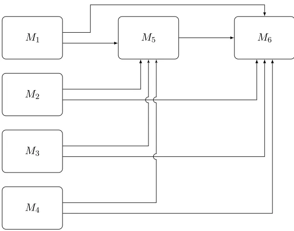
This paper examines a unit which is made up of six MOS’s,M1 -M6. M1, M2,M3, andM4 are
all MOS’s which recruit their members from a combination of NPS and AD Soldiers. Since they are two completely different populations, each group is recruited separately (that is, there are two separate recruiting goals). New recruits for these MOS’s must complete a rigorous series of prerequisites (referred to as “attrition events”) before they can even begin their MOS specific training. The attrition events are inherently different for each GT. For example, NPS recruits are required to complete BCT, whereas AD recruits have already completed it. As a result, the pass rates for each GT vary considerably. Recruits who successfully complete all attrition events begin their MOS training, which consists of a “pipeline” of six courses. Courses 1-3 are combined for all four MOS’s, while courses 4-6 are split out by MOS. Unlike the attrition events, the training pipeline is identical for each GT. Since the unit recruits new members for these MOS’s
1.2. THE PROBLEM CHAPTER 1. INTRODUCTION
from outside of itself,M1 -M4 are referred to as “initial entry MOS’s.” Figure 1.1 depicts this
process graphically.
Recruiting Pool
Attrition Events
Training
Pipeline Join Unit
Recruit Pass Pass
Fail Fail
Figure 1.1 New Recruit Path to Unit
M5 is an MOS which gains its members from within the unit’s M1 -M4 population after
they are promoted to E7. All members ofM1 - M5 combine to formM6 upon promotion to E8.
MOS’sM5 and M6 are referred to as “senior MOS’s” since they draw their members from the
seniorM1 - M4 population. Figure 1.2 shows how the different MOS’s interact with each other.
Not depicted in the figure are arcs for losses within each MOS (personnel who depart the unit). The unit has two primary manning goals. The first is to maintain a fill as close to 100% as possible without being over-strength. Although ideally each MOS would be filled to the same level, the unit can accept small imbalances within the MOS’s fill levels, provided the unit as a whole does not exceed a 100% fill level. The second goal is to achieve and maintain a ratio of 13 NPS to 23 AD across the six MOSs. This is the ratio that the unit’s commander determined would maximize the strengths of each GT. Although it could be debated whether this is the “optimal” ratio, that is a discussion that is beyond the scope of this paper and this paper exclusively focuses on the 13 to 23 ratio.
1.2.2 Decision Points and Current Methods
There are two primary decision points the unit has in order to achieve their manning goals. The first is deciding how many personnel of each GT to recruit annually, and the second is deciding how to split these recruits up into the four initial entry MOS’s. Once recruits join the unit within an MOS, the unit has limited recourse to affect their career path under current conditions; for example, if the unit is over-strength inM1 and understrength inM2, they cannot
just reassign personnel from one MOS into another. Of course, there are other things the unit
1.2. THE PROBLEM CHAPTER 1. INTRODUCTION
M1 M5 M6
M2
M3
M4
Figure 1.2 MOS Interactions Within Unit
can do to influence the makeup of their force, such as incorporating reenlistment bonuses to try to increase CR’s within one or more MOS’s, altering promotion rates, or attempting to increase/decrease pass rates for the attrition events and training pipeline. Ultimately, however, the only decisions that the unit can fully control is how many personnel to recruit, and how many to assign to each initial entry MOS. A given decision on both of these decision points together will be referred to as a “recruiting policy.”
In order to decide how many personnel to recruit annually, the unit currently examines everything in the aggregate (i.e., all MOS’s combined). Roughly speaking, each year they estimate the number of expected losses for the upcoming year (based on historical CR’s) to determine how many new graduates they will need. They then work backwards using training and attrition event pass rates to determine how many recruits they need to end up with that many new members. They also currently are working under the assumption that by graduating roughly a 1:1 ratio of NPS to AD, the difference in CR between the two populations will result in the desired 13 to 23 ratio. Over the past few years, this has resulted in a policy of recruiting 3000 AD and 2300 NPS personnel annually. Although this method provide them with a good way of replacing losses in the short term, it does not provide a clear picture of how what their manning will look like in the future, especially with respect to the strength of each individual MOS. Also,
1.3. THESIS STRUCTURE CHAPTER 1. INTRODUCTION
since they are primarily examining the MOS’s in the aggregate, they do not currently have a systematic way of knowing the best way to split their new recruits between the four initial entry MOS’s, which has led to largely reactive methods for assigning MOS’s to new recruits.
1.2.3 Purpose
The purpose of this research is to help the unit improve on its current methods for establishing recruiting policies in order to achieve and maintain their manning goals. In order to achieve this, the research must accomplish two main objectives. First, it must provide the unit with a modeling tool which they can use each year to give their decision makers a clear picture of how different proposed recruiting policies will affect their force in the long-term. Broadly, the tool needs to be able to analyze how different recruiting policies affect its composition over time. The tool needs to be specific enough to address the unit’s unique organization and goals, but should also be flexible enough that it can be used in the future as authorizations, manning goals, and other factors change. It also needs to be created on a medium which the unit can actually use in the future, rather than licensed software which would be inaccessible to a typical military unit. The tool also needs to have the capability to be used for “what-if” analysis, so the unit can see how changes to different parameters affect the outcomes. Secondly, once this tool is created, the research must apply it to analyze the problem and propose a recruiting policy based on the unit’s current situation.
1.3
Thesis Structure
The remainder of this paper is structured as follows. Chapter 2 discusses the data used, including data sources, data cleansing, and how the data was organized and restructured to provide input into the model. Chapter 3 discusses the approach used, how the model evolved over time, and details on how the final model works. In Chapter 4 the model is used to analyze the problem and produce a recommended recruiting policy for different scenarios. Finally, Chapter 5 provides a summary and outlines possible future work.
Chapter 2
Data Formulation
2.1
Data Used
2.1.1 Data Sources
All of the data used in this paper was provided by the Operations Research (OR) team from the unit’s Human Resource (HR) section. The data can be broadly broken down into two categories: training data, and Personnel Readiness Management (PRM) data. Training data consists of data on course pass rates, recycle rates, course lengths, etc., and was pulled from the Army Training Requirements and Resources System (ATRRS). PRM Data tracks the number of personnel assigned to the unit, continuation rates, rates of MOS change, etc., and the unit obtained this data from the Web Enlisted Distribution Assignment System (EDAS). The bulk of the data used came from these two sources, and the remainder of this section discusses how the data was provided by the unit. Section 2.2 discusses how the data was converted into the format required by the model.
2.1.2 Data Organization
The training data used can be broken down into two categories: attrition data and course data. Attrition data is data which tracks personnel who are recruited, but are “attritted” prior to beginning the training pipeline for their final assignment. For example, someone who is recruited, but is subsequently unable to achieve a minimum score on the Army Physical Fitness Test (APFT) or meet some other prerequisite would be considered to be attritted before they even began the training pipeline. Since this attrition data does not necessarily reflect an actual course that would be populated in ATRRS, the attrition data provided was the unit’s best estimates
2.1. DATA USED CHAPTER 2. DATA FORMULATION
Table 2.1 Attrition Events with Pass Rates by Graduate Type
Sequence Event GT PassRate
1 No Shows/Prerequisite Failures AD 0.95
1 No Shows/Prerequisite Failures NPS 0.52
2 APFT AD 0.85
2 APFT NPS 0.95
3 Prerequisite Course AD 0.34
3 Prerequisite Course NPS 0.52
4 PCS to Training Course AD 0.91
4 PCS to Training Course NPS 0.99
Table 2.2 Course C4 Class 14-001 Data
GT MOS IS QS IG QG IL QL
AD M1 13 11 8 8 4 2
AD M2 24 11 12 6 11 3
AD M3 5 0 5 0 0 0
AD M4 22 3 13 3 8 0
NPS M1 27 17 16 13 10 1
NPS M2 26 9 19 7 5 2
NPS M3 14 1 13 1 1 0
NPS M4 25 2 15 1 9 0
for the pass rates at the four different events which a recruit must pass prior to beginning the training pipeline. Some correspond to a specific event (i.e., APFT), while others may represent a series of tasks; the first event consists of things like completing paperwork, passing some screenings, and successfully showing up for training, for example. As discussed in Chapter 1, the pass rates are inherently different for each GT, and the events may be slightly different for each GT as well. The events and corresponding pass rates can be found in Table 2.1.
The course data was all pulled from ATRRS, and consists of data on the six different courses in the training pipeline which a recruit must pass prior to joining the unit. This includes two years of data for classes ending between October 1, 2013 and September 30, 2015. For each class
kof each course i, the data shows the number of first time (initial) and recycle starts, ISik and
QSik, the number of initial and recycle start graduates,IGik andQGik, and the number of first
2.1. DATA USED CHAPTER 2. DATA FORMULATION
Table 2.3 Sample of Assigned Data Format
MOS GradYr GT BASD
M1 FY14 AD 20111004
M2 FY14 AD 20090901
M3 FY07 AD 20001018
M5 FY05 AD 20021025
M6 FY02 AD 19920721
M1 FY11 NPS 20090505
M2 FY15 NPS 20120326
M3 FY14 NPS 20100803
M4 FY13 NPS 20110329
time and recycle starts with a recycle output code, ILik and QLik. An example of the data provided from one class is provided in Table 2.2.
The PRM data consists of three main categories: assigned data, CR data, and MOS change data. The assigned data is a “snapshot” of the force assigned to the unit on October 1st, 2015 which was pulled from EDAS. It contains a record for each Soldier assigned to the unit with fields for their GT, MOS, BASD, and the FY when they completed their training (i.e., when they joined the unit). A small excerpt of the thousands of records is shown in Table 2.3 as an example.
The CR data primarily consists of two fields from the past 5 fiscal years (from FY11 through FY15). The data was pulled from EDAS and contains fields for each GT/MOS/YOS combination showing how many personnel began FY iassigned to the unit (referred to as Bi), and out of those same personnel, how many were still assigned to the unit at the end of FY i(referred to asEi).
The MOS change data depicts, for the same five FY’s as the CR data, how many personnel
changed their MOS within that FY, and which MOS they changed from/to (either M5 orM6).
It contains a field for the MOS they began the FY in, and the MOS they ended the FY in. For
a given GT/MOS/YOS combination, the number of personnel who changed toM5 in FYiis
referred to asC5i, and the number of personnel who changed toM6 is referred to as C6i. A small sample of the CR and MOS change data can be seen in Table 2.4
2.1. DATA USED CHAPTER 2. DATA FORMULATION
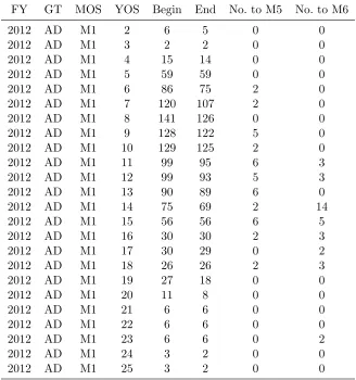
Table 2.4 Sample of CR and MOS Change Data: FY 2012 M1/AD Data
FY GT MOS YOS Begin End No. to M5 No. to M6
2012 AD M1 2 6 5 0 0
2012 AD M1 3 2 2 0 0
2012 AD M1 4 15 14 0 0
2012 AD M1 5 59 59 0 0
2012 AD M1 6 86 75 2 0
2012 AD M1 7 120 107 2 0
2012 AD M1 8 141 126 0 0
2012 AD M1 9 128 122 5 0
2012 AD M1 10 129 125 2 0
2012 AD M1 11 99 95 6 3
2012 AD M1 12 99 93 5 3
2012 AD M1 13 90 89 6 0
2012 AD M1 14 75 69 2 14
2012 AD M1 15 56 56 6 5
2012 AD M1 16 30 30 2 3
2012 AD M1 17 30 29 0 2
2012 AD M1 18 26 26 2 3
2012 AD M1 19 27 18 0 0
2012 AD M1 20 11 8 0 0
2012 AD M1 21 6 6 0 0
2012 AD M1 22 6 6 0 0
2012 AD M1 23 6 6 0 2
2012 AD M1 24 3 2 0 0
2012 AD M1 25 3 2 0 0
2.2. DATA PREPARATION CHAPTER 2. DATA FORMULATION
2.2
Data Preparation
2.2.1 Data Cleansing
The first step in preparing the data for use within the model was to scrub the data thoroughly for errors or unique outliers which could affect the model. The training data was fairly straightforward and did not require any changes. The PRM data, however, was very complicated and required certain assumptions and slight modifications to be made.
The YOS for both the CR and assigned data ranged from 0 to 32 years; however, the sample size for 0 and 1 YOS was extremely small, since it typically takes at least two years of training before a Soldier joins the unit. Therefore, data for Soldiers assigned to the unit with 0 or 1 YOS was not considered. Additionally, based on the Army’s current Qualitative Service Program (QSP) guidelines, all Soldiers E7 and below must separate upon reaching 25 YOS, and Soldiers E8 and above must separate upon reaching 31 YOS (ALARACT 066/2012). Although there are a few exceptions to these rules, the result was that there were essentially zero M1 −M5
Soldiers with more than 25 YOS, and likewise essentially zero M6 Soldiers with beyond 31 YOS.
So the few data points which violated these rules were also removed. Finally, sinceM5 requires
a Soldier to be an E7, based on the time required to achieve that rank there were no data points forM5 Soldiers with fewer than six YOS, and similarly there were no data points for M6 with
fewer than 11 YOS. The end result was CR and assigned data forM1−M4 ranging from 2 to
25 YOS,M5 for 6 to 25 YOS, and for M6 from 11 to 31 YOS. The same ranges of YOS were
used for the assigned data, which resulted in removing only three personnel with 32 YOS from the data.
Additionally, although there was ample CR data for AD Soldiers of all possible MOS’s and YOS, the CR data for NPS Soldiers was limited for certain MOS/YOS combinations. Specifically, since the unit only began recruiting NPS personnel within the last 13 years, there was very limited data for advanced YOS. From 2-11 YOS, there were a reasonable number of data points for each MOS and YOS combination to reasonably calculate the corresponding CR, but at 12 YOS that number dropped off and did not yield consistent results. For example, even in the data from the most recent fiscal year (FY14-15), there was only a total of 28 NPS personnel who began the year with 13 YOS across all six MOS’s. Discussing the lack of data with the unit, it was determined that the best solution would be to use the AD continuation rates for the NPS population with 12 or more YOS forM1−M5. This decision was based on their experience
combined with the intuition that by the time a Soldier has 12 YOS there should be minimal difference in retention behavior whether they originally came from the NPS or AD populations.
2.2. DATA PREPARATION CHAPTER 2. DATA FORMULATION
For the NPSM6 Soldiers, the sample size was similarly very small, so the ADcontinuation rates
were used for all NPS M6 Soldiers.
2.2.2 Converting to Model Input
We now briefly discuss the calculations used to convert the raw data into input for the model. For details on the format required for the input, please see Appendix A, but for the time being it is sufficient to understand that the raw numbers need to be converted into two spreadsheets for model input, referred to as thePRMtbl and theTrainingRatestbl. ThePRMtbl consists of 9 fields. The unique identifier (or Primary Key (PK)) consists of the first three fields: MOS,GradType, andYOS. For each unique record, the following data fields are required:Assigned,CR,M5R,M6R, GradDist, and PSADist. TheTrainingRatestbl consists of seven fields. The PK for this table consists of four fields: CourseNo,GradType,MOS, andAttempt. In this table, each unique record requires data fieldsPassRate,RecycleRate, andStudents. The remainder of this section discusses how each of the data entries were populated for the model input.
For the PRM input, the field Assigned simply contains the number of Soldiers assigned to the unit on October 1st, 2015 and the entries were pulled directly from the EDAS snapshot. For
the CR field, which shows the CR for a given record, the CR data for each FY was weighted
purely based on the size of its population; no extra weight was given to more recent FY’s. This method was used for two main reasons. First, based on discussion with the unit and examining the data provided, there appears to be little change in CR from one year to the next. Second, so many external factors play into retention that there is no reason to believe that any trend seen over the past 5 years within retention rates will continue or be predictive of changes going forward. So rather than risking letting any small changes that may exist within the data seriously affect a long-term model of the process, it was decided to only base each FY’s weight based on its population size (in essence, combining all of the FY’s into one). If Bi is the number assigned at the beginning of FYiandEi be the number assigned at the end of FY ifor a given GT/MOS/YOS combination, then the actual calculation for each record’s CR can be found in Equation 2.1. CR= 15 P i=11 Ei 15 P i=11 Bi (2.1)
The same logic was used in calculating the MOS change rates toM5 andM6 (fieldsM5Rand
M6R, respectively). The MOS change rates for a given record indicates the percent of personnel
2.2. DATA PREPARATION CHAPTER 2. DATA FORMULATION
within that record who changed to that MOS. It should be noted that personnel who changed MOS are still assigned to the unit, and therefore are included in the CR data as remaining in the unit, so the CR’s calculated above only represent personnel staying in the unit, not necessarily the number of personnel remaining within a given MOS. The calculation of MOS change rates for each record then is shown in Equation 2.2 and Equation 2.3.
M5R=
15
P
i=11
C5i
15
P
i=11
Bi
(2.2)
M6R=
15
P
i=11
C6i
15
P
i=11
Bi
(2.3)
The GradDist field in the PRM table contains the percent chance for a given record that a new graduate in that GT/MOS combination will have that record’s YOS when they graduate. Since all new graduates are in M1−M4, this field is 0 for allM5 andM6 records; meanwhile
these entries sum to 1 for each GT/MOS combination forM1−M4. This was calculated from
the October 1st, 2015 EDAS snapshot by subtracting each Soldier’s BASD from when they completed their training. Only the FY for when the training was available, so the date used for all calculations was the last day of the FY, since the model cycles annually.
Finally, the PSADist field shows, for AD personnel only, the distribution of PSA gains into the various records. The sample size for the PSA personnel was very small, and the unit did not have a reliable way to pull historical information about PSA personnel from EDAS. After discussing with the unit, it was estimated that PSA gains distribute evenly into the four initial entry MOS’s, and all enter with 10 YOS. The final PRMtbl input can be found in Table B.28.
For the TrainingRatestbl, two primary model inputs needed to be derived: the pass rate
Pij, and the recycle rate Rij for each course iand attempt numberj with i={1,2, ...,6}and
j={1,2,3}. Calculating the pass rates was straightforward and achieved using Equations 2.4 and 2.5, wherekrefers to the individual class number andnrefers to the number of classes with available data (this number was not necessarily the same for each course). Note that since the data pulled from ATRRS does not differentiate between second and third time starts, instead labeling them all as recycle starts, the pass rate for both second and third time starts is the same.
2.2. DATA PREPARATION CHAPTER 2. DATA FORMULATION
IPi = n P k=1 IGik n P k=1 ISik (2.4)
QPi = n P k=1 QGik n P k=1 QSik (2.5)
Calculating the recycle rate was not quite as straightforward. For first time recycles, it initially appears that you can divide the number of recycle outputs by the number of first time starts. However, discussions with the unit revealed that not all students who receive a recycle output code in ATRRS actually re-attempt the course. So although this number can be used as an estimate, it may not be completely accurate. To deal with this issue, the unit has developed a “ratio method” to calculate the recycle rate, which has proven accurate in the past, and is adopted for this paper. By assuming that over a period of time the unit has achieved a “steady state” in the ratio of first time, second time, and third time starts in each course, they are able to use the ratios of starts in conjunction with the recycle rates to estimate the true recycle rate. This is done as follows. First, define RP1 and RP2 to be the percent of recycle starts which are
on their first recycle attempt and second recycle attempt, respectively. These can be calculated for a given record using Equations 2.6 and 2.7.
RP1 =
n P k=1 ILk n P k=1
ILk+ n
P
k=1
QLk
(2.6)
RP2 =
n P k=1 QLk n P k=1
ILk+ n
P
k=1
QLk
(2.7)
Next define SPi to be the percent of a given class who is on their ith attempt. These can be calculated via Equations 2.8, 2.9, and 2.10. SPi then is the ratio of a given course whose students are currently on attempti. These can be used to calculate the approximate first time recycle rateR1 by dividingSP2 bySP1, and similarly find the approximate second time recycle
rateR2 by dividing SP3 bySP2 as in Equations 2.11 and 2.12. Also, since only 3 attempts are
allowed, it follows thatR3= 0.
2.2. DATA PREPARATION CHAPTER 2. DATA FORMULATION
SP1=
n P k=1 ISk n P k=1
ISk+ n
P
k=1
QSk
(2.8)
SP2=RP1
n P k=1 QSk n P k=1
ISk+ n
P
k=1
QSk
(2.9)
SP3=RP2
n P k=1 QSk n P k=1
ISk+ n
P
k=1
QSk
(2.10)
R1 =
SP2
SP1
(2.11)
R2 =
SP3
SP2
(2.12)
Finally, theStudents field of the TrainingRatestbl simply holds the number of students who were currently in a given course/attempt on October 1st, 2015. Unfortunately, the unit was not able to get this data from ATRRS as originally planned, so an estimate was used which is discussed in Chapter 4, and the field remains 0 for all records in the table, but the field was kept to provide this functionality within the model for the unit going forward.
2.2.3 Additional Model Inputs/Assumptions
In addition to the two primary model input tables discussed in section 2.2.2, some additional estimates were provided to the model as well. As mentioned earlier, the attrition events were entered into the model directly, as shown in Table 2.1. Additionally, authorizations for each MOS were entered directly into the model, which were provided by the unit. Also entered into the model directly are the course numbers, course names, the length of each course (in weeks), and the recycle delay for each course (in weeks), which was pulled from ATRRS. These are used later to calculate how long a new recruit is expected to be in training before becoming available to the unit.
Finally, another spreadsheet referred to as theTrainingDelaytbl was needed as a model input. This table consists of only three fields. The PK is the combination of theGradType and Delay
2.2. DATA PREPARATION CHAPTER 2. DATA FORMULATION
fields, which represent the non-course related delay (in weeks) from the beginning of a FY and when a recruit is expected to be available to the unit. The Prob field contains the probability of a given delay. A uniform distribution was assumed, ranging from 32-108 weeks for AD and from 32-84 weeks for NPS. These delays include things such as the time it takes the recruiters to actually sign up a recruit, next available course date, the time for various attrition events, and time for a Permanent Change of Station (PCS) from a Soldier’s current duty station to the unit.
Chapter 3
Modeling
3.1
Model Development and Basic Reports
3.1.1 Initial Approach
The first step in modeling the problem was to determine what type of model would most accurately represent the problem while achieving the goals discussed in Chapter 1. Since the goal was to create a tool which can be easily used and updated by the unit going forward, it was decided to limit the use of software to the Microsoft Office Suite, which the unit has available and is familiar with. Microsoft Access was chosen as the interface because of its ability to build user-friendly forms and easily handle the data sets in an organized manner. Coding was done in VBA because of its simplicity and ability to interact seamlessly with Microsoft Access.
With the tool’s medium determined by necessity, the next step was to decide how to model the problem. As discussed in Section 1.2.2, the primary focus was on informing the unit in support of their two primary decisions: how many personnel to recruit annually, and how to distribute these recruits between the four initial entry Military Occupational Specialties (MOS). Since the unit makes these decisions annually, it was decided to make the process discrete by Fiscal Year (FY). This also aligns with the Continuation Rate (CR) and other data provided by the unit, as discussed in Chapter 2. Additionally, since VBA has some limitations compared to more powerful software, a model was needed which would not be overly demanding computationally. As a result, it was decided to model the process deterministically. The model would project the “flow” of personnel through the organization over time, including personnel who were recruited but never actually joined the unit (i.e., were attritted during attrition events or during the training pipeline). The initial concept, then, was to build a model which would allow the user to
3.1. MODEL DEVELOPMENT AND BASIC REPORTS CHAPTER 3. MODELING
input a recruiting policy, and using historical attrition rates, training rates, continuation rates etc., would provide a report with the unit’s projected composition at the end of each Fiscal Year (FY) for a given period of time. The model itself was not intended to recommend recruiting policies, but rather serve as a tool to evaluate potential policies the unit is considering. The following section shows how the model was developed and changed over time.
Probably the most important part of developing the model was ensuring that it provided the unit with the information they would need going forward. In light of this, rather than trying to build a final product from the beginning, the process was first broken down into different pieces, getting feedback from the unit, and then assembling the different parts into a whole. The process can be logically broken down into two parts: the time before a new recruit joins the unit as they navigate the attrition events and training pipeline, and the time after they join the unit. These two stages are referred to as the training phase and the available phase, respectively. To model each phase, a “report” was built which provided detailed analysis of that phase, with the goal of later combining them to model the entire process. Sections 3.1.2 - 3.1.4 introduces the reports that were built to model each phase, explains how they work, and outlines how the unit’s feedback was used to improve them. Section 3.2 details how they were combined to model the entire process.
3.1.2 Report 1: Single MOS Report
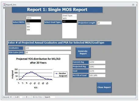
The starting point for modeling the available phase was a simple report to examine one initial entry MOS at a time. Report 1 was designed to provide the unit with the projected Years of Service (YOS) distribution at the end of a period of time for a user-selected MOS and Graduate Type (GT), given a projected number of annual graduates for that MOS and GT. To run the projection, the user selects an initial entry MOS and GT, and enters a length for the projection, number of projected annual graduates (for that MOS/GT only), and for Active Duty (AD) the number of projected annual PSA gains for that MOS. Figure 3.1 shows an example of the report, where the user has selected a 20 year projection for Active Duty M1 personnel, given 100 annual
graduates and 5 annual PSA gains. The graph shows the projected YOS distribution at the end of the 20 years. The textboxes to the right of the graph display various information provided by the report: “Current Asg” shows the number ofM1/AD personnel currently assigned to the unit
(as of October 1st); “Projected Asg” shows the projected total number of M1/AD personnel
that will be assigned to the unit after 20 years; “Goal” shows the goal fill forM1/AD (number
authorized times the desired AD percent); “Pct Fill of Goal” shows the projected percent of the goal that will be assigned. These outputs let the unit quickly see what a given number of
3.1. MODEL DEVELOPMENT AND BASIC REPORTS CHAPTER 3. MODELING
annual graduates for one MOS/GT would result in, either in the short term or after achieving a steady state.
Figure 3.1 Report 1: Projected YOS distribution and total assigned for M1/AD at the end of 20 years, given 150 annual graduates and 10 annual PSA gains
Report 1 works following the logical steps outlined in Figure 3.2. First, it retrieves the number of personnel assigned for the selected MOS/GT at the start of the current FY from
the table PRM tbl as a starting point (broken down by YOS). It then uses the continuation
rates and MOS change rates also found inPRM tbl to “advance” the personnel assigned by one year. This involves removing losses from the MOS (whether due to leaving the unit or MOS change) and increasing the YOS for everyone remaining in the unit by 1. It then adds in the number of annual graduates (provided by the user) and distributes them into the available force
3.1. MODEL DEVELOPMENT AND BASIC REPORTS CHAPTER 3. MODELING
based on the distribution found in theGradDist field of PRM tbl, before finally adding in the user entered number for annual PSA gains (if applicable) and inserting them according to the PSADist field of PRM tbl. The second and third steps of this process repeat for as many years as the user requested.
1. Get Current Assigned
2. Advance Personnel
1 Year
3. Add Gains
PRM tbl PRM tbl User Input,
PRM tbl
Figure 3.2 Report 1 Model Process
The calculations for steps two and three were conducted as follows. For a given GT, letAi,y,t be the number of personnel assigned of MOSMi withyYOS at the start of FYt. ThenAi,y+1,t+1
can be calculated using Equation 3.1, where CRi,y, M5Ri,y, andM6Ri,y are the Continuation
Rate, MOS change rate to M5, and MOS change rate toM6 for MOS Mi with y YOS; Gi is
the number of annual graduates for MOS Mi;gi,y is the probability of a new graduate of MOS
Mi having y YOS at graduation;P SAi represents the number of PSA gains for MOS Mi; and
pi,y represents the probability of a PSA gain in MOS Mi having y YOS upon re-entry into the unit. Recall from Chapter 2 that for the initial entry MOS’s, 2≤y≤25, soAi,2,t+1 will only be
populated by new graduates.
Ai,y+1,t+1 =Ai,y,t(CRi,y−M5Ri,y−M6Ri,y) +Gi·gi,y+1+P SAi·pi,y+1Ai,y,t (3.1)
The unit’s feedback on Report 1 was positive overall, as it achieved its goal of providing a visualization of the YOS distribution for the different MOS’s and GT’s, and facilitated quickly determining the number of annual graduates needed to attain a certain fill within an MOS. That being said, on its own the report is of somewhat limited value since it does not depict the interaction between the initial entry and senior MOS’s, and does not allow the user to view multiple MOS’s at the same time. Since the report was largely built as a “stepping stone”
3.1. MODEL DEVELOPMENT AND BASIC REPORTS CHAPTER 3. MODELING
towards Report 2, it did not evolve very much during the process and instead its shortcomings were addressed in Report 2.
3.1.3 Report 2: Multiple MOS Report
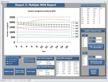
Report 2 was designed to expand on Report 1 to incorporate multiple MOS’s at the same time. Similarly to Report 1, it only examined the available phase of the process; the training phase was overlooked. For Report 2, the user enters the length of the projection (in years), the number of projected annual graduates for each initial entry MOS/GT combination, and the number of annual PSA gains for each AD MOS. Figure 3.3 depicts an example of a 20 year projection with user-provided annual graduates according to the listbox at the upper-right hand of the form. The graph is showing the annual number assigned for each MOS, but can be adjusted using the toggle buttons and checkboxes below the graph to display other information as discussed below. The “Export Graph Data to Excel” button below the graph options exports the data currently shown on the graph to an excel file. The listboxes below the graph show numbers of various numbers assigned and percent fills. Inside of the black box to the right of the form, the user can update the number of AD or NPS annual gains, and re-run the report.
Report 2 works similarly to Report 1, with one important distinction. When advancing the assigned force by one year, rather than “throwing out” personnel who changed their MOS, they needed to be reassigned to their new MOS. So the logic behind the report is the same as that shown in Figure 3.2, except that Step 2 now involves simultaneously removing losses and reassigning personnel between MOS’s. For the initial entry MOS’s, then, the same calculation was used as Report 1, found in Equation 3.1. For the senior MOS’s, however, a different process needed to be followed, since they only receive their gains from the other MOS’s. Equation 3.2 and 3.3 show how M5 andM6 were advanced, respectively (using the same notation as in
Equation 3.1).
A5,y+1,t+1=A5,y,t(CR5,y−M6R5,y) +P SA5(p5,y+1) + 4
X
j=1
Aj,y,t(M5Rj,y) (3.2)
A6,y+1,t+1 =A6,y,t(CR6,y) +P SA6(p6,y+1) + 5
X
j=1
Aj,y,t(M6Rj,y) (3.3)
Unit feedback was key in developing the presentation of Report 2. First, since displaying the YOS distribution for several MOS’s at the same time would be cumbersome, the report also instead showed the total number of the different MOS’s over time. Initial versions of the report
3.1. MODEL DEVELOPMENT AND BASIC REPORTS CHAPTER 3. MODELING
provided one set graph as the focal point, which displayed 12 data series (one for each MOS/GT combination). At this point however the unit made it clear that it was important for the report to be able to display the results for the aggregated totals in addition to the individual MOS’s, as well as visualizations of other data besides just the raw number assigned. To address these issues, options were added to allow the user to choose to aggregate all MOS’s and/or combine the AD and NPS numbers. Additionally, the interface was altered to allow the user to view the annual breakdown of the total assigned, percent fill, or losses. The final result displayed in Figure 3.3 was a significant improvement over the basic structure found in Report 1.
Figure 3.3 Report 2: Projected force composition based on a user provided number of annual gradu-ates of each MOS and GT.
3.1. MODEL DEVELOPMENT AND BASIC REPORTS CHAPTER 3. MODELING
3.1.4 Report 3: Training Report
With a firm handle on projecting force flow once personnel have joined the unit, the focus changed to the more challenging aspect of projecting how recruits would navigate the training phase. The goal of the report was to project, for a given number of recruits and a method of MOS distribution, how many of the recruits would graduate within each MOS. Figure 3.4 shows an example of the report where 3000 AD and 2300 NPS personnel are recruited (the unit’s current recruiting numbers), and an authorizations-based method of MOS distribution is used (details on that below). The listboxes to the right of the report show the total number of graduates of each GT, the MOS distribution of the recruits for each GT, and the number of graduates by MOS and GT. The bar graph depicts the distribution of when graduates of each MOS/GT combination will be available (in this case, all will require 2-4 years of training before they join the unit).
In order to develop the report, it was necessary to calculate the rate at which recruits who would successfully complete the attrition events and training pipeline, determine a way to distribute recruits into the four initial entry MOS’s, and also calculate how long the process would take for recruits to navigate the entire process and join the unit. The problem was simplified by treating the training phase as being broken into three parts: attrition events, combined MOS courses, and MOS specific courses. Although the actual decision of assigning MOS’s may occur before a recruit begins the training pipeline, the model was further simplified by making this decision after completion of the combined MOS courses. The AD and Non-Prior Service (NPS) populations were treated completely separately, so for the rest of this section all calculations are assumed to be for one given GT.
Since the Attrition Events are treated as one time “pass/fail” events with a given pass rate provided by the unit, calculating the number of recruits projected to pass them was done by multiplying the number of recruits times each of the rates successively, as in Equation 3.4 where
PA,trepresents the number of yeartrecruits projected to pass the attrition events,Rtrepresents the number of year trecruits, and ai represents the pass rate for attrition eventi.
PA,t=Rt
4
Y
i=1
ai (3.4)
Calculating the pass rate for the combined MOS portion of the training pipeline required taking into account the possibility of recycling individual courses. This was accomplished for each course by adding the probabilities of graduating in one, two, or three attempts to obtain a course pass rate, and then multiplying the three combined MOS course pass rates to obtain an
3.1. MODEL DEVELOPMENT AND BASIC REPORTS CHAPTER 3. MODELING
Figure 3.4 Report 3: Projected graduates and availability for 1000 AD and 1000 NPS recruits using authorizations-based MOS distribution
3.1. MODEL DEVELOPMENT AND BASIC REPORTS CHAPTER 3. MODELING
overall pass rate for the combined MOS courses. Equation 3.5 shows how the calculations were completed, where PC,t represents the number of yeartrecruits to complete the combined MOS courses,pj,k represents the pass rate for course j on attempt k, andrj,k represents the recycle rate for course j on attemptk.
PC,t=PA,t
3
Y
j=1
(pj,1+rj,1pj,2+rj,1rj,2pj,3) (3.5)
Given a number of recruits R for a given GT, the above calculations provided how many
were projected to be available to assign to the MOS specific courses for M1, M2, M3,and M4.
The process of MOS distribution will be addressed later; for now assume that MOS Mi was
assigned PC,t(di,t) personnel, where di,t is the distribution of students for MOS Mi for year t recruits. Then calculating the number of graduates for yeartrecruits for Mi, denoted Gi,t, is accomplished using Equation 3.6, lettingpi,j,k and ri,j,k represent the pass and recycle rates for MOS ifor coursej on attemptk. The product portion of the right hand side of this equation (the pass rate for the MOS specific courses for MOSMi) is denoted by zi.
Gi,t=PC,t(di,t)
6
Y
j=4
(pi,j,1+ri,j,1pi,j,2+ri,j,1ri,j,2pi,j,3) (3.6)
The next step was to address how to determine the distribution used to populate di,t. Since this was one of the key decisions available to the unit, it was important to come up with a method that would keep them as close as possible to having a 100% fill for each MOS. After a series of discussions with the unit, it was decided to provide three different methods for distributing students into the four MOS’s: the manual entry method, the authorizations-based method, and the current shortages method. The manual entry method is exactly what its name implies: the user manually enters a value for each di,t. The authorizations-based method distributes students based on the ratio of each MOS’s authorizations to the sum of the initial entry MOS authorizations, as in Equation 3.7. Note that these two methods maintain the same value for all
t, so thatdi,j =di,k for any j and k.
di,t =
Mi authorizations
4
P
j=1
Mj authorizations
(3.7)
In addition to the first two basic options, it was desired to provide an option which would utilize an algorithm to determine the MOS distribution based on the unit’s current composition,
3.1. MODEL DEVELOPMENT AND BASIC REPORTS CHAPTER 3. MODELING
which is the purpose of the current shortages method. The current shortages method aims to populatedi,t based on the unit’s current assigned, projected gains (current students who are projected to graduate in each MOS), and the relative difficulty of MOSMi’s MOS specific courses
(i.e., how many of those assigned to Mi are projected to actually graduate). The following
algorithm takes these factors into account. First, define ∆i using Equation 3.8. Here, Vi,t represents the AD/NPS ratio goal-adjusted authorizations forMi (i.e, for AD,Vi is two-thirds of the number of authorizations forMi, and for NPS, Vi is one third the number of authorizations forMi). So greater values for ∆i,t indicate greater shortages forMi at timet, adjusted for future graduates.
Get ∆i’s Fill to
even ∆i’s
Distribute Remaining Students PRM tbl,
Grads tbl zi’s zi’s
Figure 3.5 Current Shortages Method Algorithm
∆i,t =Vi,t−
∞
X
k=t+1
Gi,k−
25
X
y=2
Ai,y,t (3.8)
Once ∆i,t is calculated for all four initial entry MOS’s, the algorithm works as follows (see Figure 3.5 for visualization). First, identify the ∆j,t and ∆k,t with the greatest and second greatest values, respectively. Then, assign xj personnel to ∆j,t according to Equation 3.9. Once this is done, ∆j,t= ∆k,t. The reasoning behind dividing byzj is that ∆ is measured in terms of
personnel assigned to the unit and projectedgraduates, not number of students, so the MOS
specific pass rates need to be taken into account. When this is complete, identify the ∆m,t
with the third highest value, and assign personnel to both Mj and Mk using the same logic
as in Equation 3.9 so that ∆j,t = ∆k,t = ∆m,t, and then repeat the process to bring them
all to the level of the ∆ with the lowest value. Once this step in the algorithm is complete, ∆1,t = ∆2,t = ∆3,t= ∆4,t; in other words, all of the MOS’s will be filled equitably. The remaining
s students are then distributed so that each MOS Mi is assignedyi students such that each
3.1. MODEL DEVELOPMENT AND BASIC REPORTS CHAPTER 3. MODELING
MOS is projected to receive the same number of additional graduates, as in Equation 3.10.
xj = 1
zj
(∆j,t−∆k,t) (3.9)
yi =s
1 zi 4 P j=1 1 zj (3.10)
These procedures calculated the number of projected graduates for each initial entry MOS for a given number of recruits and user selected method of MOS distribution. The next step was to calculate when those graduates would be available, or in other words, how long the delay would be from the time the recruits were requested (October 1st of each FY) until they would actually join the unit. The delay needed to include the time it takes for recruiters to go out and find the recruits, the time it takes the recruits to complete the attrition events and PCS to the training pipeline, and the time it takes them to complete the training pipeline. The first two portions were estimated in conjunction with the unit outside of the model and input into the table TrainingDelay tbl, as explained in Section 2.2.3. To calculate the time spent in the training pipeline, the first step was to enumerate every possible “path” a student could take to complete the six training courses. For example, a student could pass all six on the first attempt, or they could pass courses 1-5 on the first attempt, and pass course 6 on the second attempt, etc. Since each course allows a maximum of three attempts, this resulted in 36 or 729 paths a
student could take to graduation. A path for MOS Mi can be denoted as a 6 element vector
vi,π, whose jth entry, vi,π(j) represents the number of attempts a student on path π requires to pass course j. This notation implies that vi,π(j) ∈ {1,2,3} ∀i, j. Using this notation and remembering thatpi,j,k represents the probability of a student of MOS ipassing coursej ink attempts, it was possible to calculate the probability of a student with MOS Mi following a given path,P(vi,π), using Equation 3.11. The probabilities were normalized by dividing by their sum since the goal was to only calculate the delays for students who will graduate.
P(vi,π) =
6
Q
j=1
pi,j,vi,π(j)
729 P γ=1 6 Q j=1
pi,j,vi,γ(j)
(3.11)
The number of weeks a given path vi,π would take was calculated by summing the length
of each course and the appropriate number of “recycle delays” for the course, which was also
3.2. REPORT 4: FORCE PROJECTION REPORT CHAPTER 3. MODELING
discussed in section 2.2.3 and found in the table Courses tbl. The number of weeks spent on coursejifkattempts are needed is denoted aswj,k, and can calculate the total number of weeks needed for a given path, W(vi,π), using Equation 3.12.
W(vi,π) =
6
X
j=1
wj,vi,π(j) (3.12)
The next step was to add the non-training delays to each of these calculated delays. Since the analysis assumed the non-training course delays were uniformly distributed, the distribution is defined by the minimum and maximum values aandb respectively. Then the total delay (in weeks) for a given path vi,π is also uniformly distributed as in Equation 3.13.
D(vi,π)∼U(a+W(vi,π), b+W(vi,π)) (3.13)
With all delays now accounted for, the probability weighted sum of the distributions for each path was used to obtain a total delay distribution. Finally, all that needed to be done was to take that and divide its values by 52 and then round up to convert the delay into years to obtain a final delay distribution in years, Yi, for MOS Mi. Making all of the above calculations turned out to be quite time consuming and made the model run slowly, so rather than recalculate them every time the report was run, the delay distributions were calculated once when a new TrainingRates tbl or TraininDelay tbl was imported, and the results were stored in the table GradProb tbl.
With all of the calculations completed, the model could provide both the projected number of graduates for each MOS and when they would be available, based on the number of recruits input by the user. The focal point of the report is the graph showing by MOS and GT the expected number of graduates for each year. The unit approved of Report 3’s layout, since although the calculations were more involved than the other reports, its real purpose was to simply display projected number of graduates.
3.2
Report 4: Force Projection Report
3.2.1 Report Development
Although the reports discussed in Section 3.1 are useful for analyzing the individual parts of the process in detail, the most useful tool we could provide the unit would be one which analyzed the whole process at once. Report 4, the “Force Projection Report,” addresses this need by
3.2. REPORT 4: FORCE PROJECTION REPORT CHAPTER 3. MODELING
essentially combined the logic of the first three reports to model both the training and available force phases; Report 4’s logical steps are shown in Figure 3.6. Step 3 followed the logic used in Report 3, and Steps 4 and 5 followed the logic from Report 2, so they will not be discussed in detail here; instead the focus will be on steps 1, 2, and 6.
1. Get user input
2. Calculations for current students
3. Calculate gains for current year recruits
4. Advance per-sonnel 1 year
5. Distribute gains into unit
6. Output Results
Figure 3.6 Report 4 logical flow; steps 3-5 are repeated for each year of the projection.
Step 1 involves getting the parameters for the projection from the user. Initial versions of Report 4 only allowed the user to select the length of the projection, the number of annual recruits and PSA gains, and the method of MOS distribution. When presented to the unit, they expressed the desire to be able to use the report to compare multiple recruiting policies at one time. Additionally, they wanted to be able to use it for “what if” analysis, for example seeing how the projection would change if AD continuation rates were increased by 1%, or if MOS