DOI: 10.1534/genetics.104.030171
Maximum-Likelihood Estimation of Demographic Parameters Using the
Frequency Spectrum of Unlinked Single-Nucleotide Polymorphisms
Alison M. Adams*
,1and Richard R. Hudson
†*Committee on Genetics and†Department of Ecology and Evolution, University of Chicago, Chicago, Illinois 60637
Manuscript received April 17, 2004 Accepted for publication July 13, 2004
ABSTRACT
A maximum-likelihood method for demographic inference is applied to data sets consisting of the frequency spectrum of unlinked single-nucleotide polymorphisms (SNPs). We use simulation analyses to explore the effect of sample size and number of polymorphic sites on both the power to reject the null hypothesis of constant population size and the properties of two- and three-dimensional maximum-likelihood estimators (MLEs). Large amounts of data are required to produce accurate demographic inferences, particularly for scenarios of recent growth. Properties of the MLEs are highly dependent upon the demographic scenario, as estimates improve with a more ancient time of growth onset and smaller degree of growth. Severe episodes of growth lead to an upward bias in the estimates of the current population size, and that bias increases with the magnitude of growth. One data set of African origin supports a model of mild, ancient growth, and another is compatible with both constant population size
and a variety of growth scenarios, rejecting greater than fivefold growth beginning⬎36,000 years ago.
Analysis of a data set of European origin indicates a bottlenecked population history, with an 85%
population reduction occurringⵑ30,000 years ago.
P
ATTERNS of genetic variation in contemporary to be statistically independent of each other and the data are completely characterized by the number of populations can be used to make inferences aboutpast population size changes. Ideally, likelihood meth- polymorphic sites and the frequency spectrum. That is, we can represent the full data bym⫽(m0,m1,m2,mn⫺1),
ods using the full data would be applied to make such
inferences. For the case of DNA sequence polymorphism where m0 is the number of sites monomorphic in the
sample, and, fori⬎0,miis the number of polymorphic and where no recombination occurs between the
vari-sites in which the derived allele is presentitimes in the able sites, methods are available for carrying out such
sample ofnchromosomes. We assume all polymorphic inferences (BeerliandFelsenstein2001;Kuhneret al.
sites are biallelic. Then,兺n⫺1
i⫽0miisL, the number of sites
1998;Nielsen1999). With incomplete linkage between
surveyed, and兺n⫺1
i⫽1miis the total number of segregating
sites, such approaches are frequently computationally
sites in the sample,S. Also note thatm0⫽L⫺S. In this
infeasible. An exception is the case in which only two
case of free recombination between sites, full-likelihood chromosomes are sampled at each locus, whereMarth
approaches are computationally undemanding. This case
et al.(2003) have shown that maximum-likelihood
meth-has been examined by Wooding and Rogers (2002), ods are feasible. These computational difficulties have
PolanskiandKimmel(2003), andMarthet al.(2004) led to the use of summary statistics such as Tajima’sD
and is also the focus of our study. We examine the (Tajima1989) for making inferences about past
demog-statistical properties of demographic inferences based raphy. For example,WallandPrzeworski(2000) and
on m, using maximum likelihood and assuming sites
Pluzhnikovet al.(2002) tested compatibility between
are independent. By utilizing the entire frequency spec-observed values of Tajima’s D and values observed in
trum,m, rather than a summary statistic such as Tajima’s simulations under constant-size and alternative
demo-D, this approach captures all available information in graphic scenarios.WeissandVon Haeseler(1998) also
data sets consisting of unlinked polymorphic sites. focused on summaries of the data by implementing a
With linkage between sites, there is a statistical nonin-likelihood approach based on mean pairwise differences
dependence between polymorphic sites, and thusmfor and segregating sites for a model of complete linkage.
a set of linked sites would contain less information than With free recombination between sites, the problem
that for a set of unlinked sites. It follows that our results is greatly simplified. In this case, sites can be considered
for unlinked sites give an idea of the best one can do usingmor summary statistics, such as Tajima’sD, which can be calculated from it. It is important to note that
1Corresponding author:Department of Ecology and Evolution, 1101
for linked sitesmdoes not completely characterize the
E. 57th St., Room Z302, University of Chicago, Chicago, IL 60637.
E-mail: [email protected] data, and that full likelihood, which incorporates
equal to one or to the case of a population reduction with no recovery by setting frec equal to fint. We also
assume that the population is unstructured (panmictic) and that the polymorphic sites are unlinked.
Maximum-likelihood method: The maximum-likeli-hood approach followed here is that ofWoodingand
Rogers(2002) andPolanskiandKimmel(2003). Our
Figure1.—Demographic model.fint(⫽Nint/N0),frec(⫽Nrec/
N0), andTare the estimated parameters. analyses require a population survey of variation at a
set ofLunlinked sites. ForLunlinked sites,mis multi-nomially distributed,
formation about linkage disequilibrium, for instance,
might result in better inferences. Prob(m)⫽
冢
Lm0 m1 . . . mn⫺1
冣
兿
n⫺1i⫽0 Pmi
i , (1)
The models examined here consist of either exponen-tial growth or an instantaneous decrease followed by
where P0is the probability that a site is monomorphic
exponential growth, which requires simultaneous
esti-in the sample, and, fori⬎ 0,Piis the probability that mation of either two or three parameters, respectively.
a site is polymorphic withicopies of the derived allele. We illustrate that, particularly for recent growth
scenar-The Pi’s are functions of the four parameters of the ios, data sets consisting of large numbers of segregating
demographic model (0,fint,frec, andT) and the sample
sites are required to produce good estimates based solely
sizen. on frequency spectrum data. Our results provide a
theo-To obtain the maximum-likelihood estimates of the retical perspective on the feasibility of frequency
spec-parameters one maximizes the right-hand side of (1). trum-based parameter estimation with a modest amount
We note, however, that we can write the probability of of data, and we present methods to determine the
ap-the data as proximate variance and covariance associated with such
estimators under any demographic scenario of interest.
Prob(m)⫽
冢
Lm0 m1 . . . mn⫺1
冣
P (L⫺S)0 (1⫺P0) S
兿
n⫺1
i⫽1
Pmi
i
(1⫺P0)mi
The maximum-likelihood method is also applied to
three human data sets. The first is an African data set (2) consisting of the original data set ofFrisseet al.(2001)
⫽
冢
m L0 m1 . . . mn⫺1
冣
P (L⫺S)0 (1⫺P0) S
兿
n⫺1
i⫽1
pmi
i , (3)
as well as 40 additional locus pairs (A.Di Rienzo, unpub-lished data). The Seattle single-nucleotide polymorphisms
where pi (⫽ Pi/(1⫺P0)) is the probability that a site
(SNPs) data, consisting of both African-American and
Eu-is polymorphic withicopies of the derived allele, condi-ropean data sets (http://pga.gs.washington.edu), is also
tional on the site being polymorphic in the sample.P0
examined. Each of these data sets consists of linked
and the pi’s can be written in terms of 0 and mean
segregating sites within effectively unlinked loci, and a
properties of sample gene trees. For example, for small procedure is outlined by which one can extend this
0,P0can be expressed in terms of the mutation
parame-method to such data and construct the appropriate
con-ter and the mean total length of the gene genealogy, fidence regions associated with the estimators.
P0⬇1⫺ 0(n), (4)
MODEL AND METHODS where(n) is the mean total length of the gene tree of
a sample ofn chromosomes measured in units of 4N0
Model: The demographic model considered is that
generations (Hudson1990). We define ani-branch to of a population of constant effective sizeN0until time
be a branch of the gene tree such that a mutation that
Twhen there was an instantaneous decrease to an
in-occurs on the branch results inicopies of the mutation termediate population size (Nint) followed by
exponen-in the sample. The mean total length ofi-branches in tial growth to the current population size (Nrec). As
illus-units of 4N0 generations we denote by i(n). Then, Pi
trated in Figure 1, this model involves four demographic
isⵑ0i(n), and
parameters: N0, Nint, Nrec, and T, where T is the time
at which the instantaneous size change occurred. Tis
pi⬇0i(n)
0(n)
⫽ i(n)
(n), i⬎0 . (5)
measured in units of 4N0 generations before the
pres-ent. We assume the mutation rate per site,u, is small,
i(n) and(n) are functions of fint,frec, and T, but do makes only a minimal difference to our results (data
not depend on N0 or 0. Thus, to find the maximum- not shown). We also assume that all sites are surveyed
likelihood estimates of the four parameters, we can first in a sample ofnchromosomes (orn/2 diploid individu-find the maximum-likelihood estimates,fˆint,fˆrec, andTˆ, als), but more general sampling is easily accommodated.
by maximizing
兿
n⫺1i⫽1pmii. The maximum-likelihood estimate For example, one can separate a data set into a series
of frequency spectra, each with a differentn. A global of0, if desired, can then be obtained as ˆ0 ⫽ (S/L)/
ˆ(n), whereˆ(n) is the mean gene tree length withfint, likelihood may then be obtained for the entire data set frec, and T set equal to the maximum-likelihood esti- by multiplying the result of Equation 6 for sets of sites
mates. In this article, we focus on estimation of the param- with different sample sizes. etersfint, frec, and T, which requires maximizing
兿
n⫺1
i⫽1pmii Sample size comparison: We compare the effect of
sample size and number of unlinked polymorphic sites and does not require specifying Lor m0. Equivalently,
we can consider estimation of the parameters based on on both the power to reject the null hypothesis of con-the probability ofmconditional onS, which is stant population size and the quality of estimates of specific demographic parameters. The number of segre-Prob(m|S)⫽Prob(m)
Prob(S) gating sites, when indicated, is scaled on the basis of the average total branch length of a random gene genealogy (), which will vary according to sample size and
demo-⫽ Prob(m)
冢
Lm0
冣
P (L⫺S)0 (1⫺P0)S
graphic scenario. For example, suppose we wish to com-pare sample sizes of 50 and 100 chromosomes under a growth scenario where 40-fold expansion occurred beginning 10,000 years ago. In this case(50) (in units of
⫽
冢
Sm1 m2 . . . mn⫺1
冣
兿
n⫺1i⫽1 pmi
i , (6)
4N0 generations) for a sample size of 50 chromosomes
is 4.93,(100) for a sample size of 100 chromosomes is which does not depend onLorm0. 6.06, and(100)/(50) is 1.23. In words, the average
To find the maximum-likelihood estimates offint,frec,
total branch length of a random gene genealogy is 1.23 andT, we estimate Prob(m|S) at a set of points on a
times greater for a sample size of 100 than for a sample rectangular grid of values in the three-dimensional
size of 50. This indicates that, for every 500 segregating space of fint, frec, and T values. For each point in the
sites discovered in a sample size of 50,ⵑ615 segregating grid, we estimate thei(n)’s by generating 100,000
repli-sites would be found in a sample size of 100 if the cate gene trees with simple one-site coalescent
simula-same number of sites were sequenced. Thus, when we tions. The i(n)’s can also be obtained as described
compare sample size 50 to sample size 100, we compare elsewhere (GriffithsandTavare´1998;Woodingand
n⫽ 50,S⫽500 ton⫽100,S⫽615. Normalizing the
Rogers 2002; Polanski and Kimmel 2003), and this
number of sites in this way serves to facilitate compari-method can be generalized to any demographic model
sons between analyses of different sample size because it for which the relevanti(n)’s can be calculated or
esti-takes into account the expected number of polymorphic mated. From the estimatedi’s, thepi’s are calculated,
sites in the samples of each size. which in turn are used to calculate the product,
Asymptotic properties:To investigate whether
asymp-兿
n⫺1i⫽1pmi i. Since we have ignored the problem of
estimat-totic approximations of confidence regions and vari-ing0, we do not requireL, and the results are all given
ances of estimators are applicable to data sets of modest conditional on specified numbers of polymorphic sites.
size, we first determined whether 95% confidence
re-Required data:Our analyses require data in the form
gions obtained from the log-likelihood ratio have the of unlinked polymorphic sites. Ascertainment bias is not
expected coverage properties. Confidence regions in-considered in this article, so we assume that sites are
clude those points on the grid with a log-likelihood ratio randomly chosen with no prior knowledge of
polymor-⬍3 or 3.9 for simultaneous estimation of two or three phism and sequenced in each sampled chromosome.
parameters, respectively. We also compared the
ob-Frisseet al.(2001) sequenced ⵑ25 kb and found 120
served variances and covariances of the estimators with segregating sites in an African Hausa sample of 30
chro-the approximate variances and covariances calculated mosomes. If we consider genome-wide polymorphism
by estimating the inverse of the information matrix, levels to be similar to that data, thenⵑ104,000 sites would
have to be sequenced in 30 chromosomes to assemble
a data set consisting of 500 segregating sites. These Iij⫽ ⫺E
冢
2ij
log L
冣
. (7) 104,000 sites could be sequenced in small unlinkedseg-ments throughout the genome to obtain frequency spec- We estimate the expected log-likelihood with trum data from unlinked polymorphic sites. We
con-sider only biallelic polymorphic sites and assume that
E(logL)⫽
兺
n⫺1
i⫽1
Pi(frec0,fint0,T0)log(Pi(frec,fint,T))
the ancestral/derived status of each allele is known.
Figure2.—Power to detect growth
withⵑ500 unlinked sites. The
num-ber of sites used for each point in a curve is scaled on the basis of 500 sites in a sample size of 20. (a) Effect of sample size on power to detect re-cent growth beginning 10,000 years
ago (T⫽0.0125). (b) Effect of the
onset time of growth on power to de-tect growth with a sample size of 20.
with thePi(frec0,fint0,T0) estimated by coalescent simula- estimated from simulation, are in very close agreement
to i(n)’s calculated numerically by the method of
tion for a set of points on a narrow grid offrec,fint, and
Tvalues around the true parameter values of frec0,fint0, PolanskiandKimmel(2003). For the case offrec⫽2.0, fint⫽0.15, andT⫽0.0375 for a sample size of 46, the
and T0. The second partial derivatives relevant to the
information matrix are then approximated from best- maximum-likelihood parameters for the Seattle SNPs fit second-degree polynomial curves. The variance and European data set, we find that our simulated i(46)’s
covariance observed from simulation can then be com- differ, at most, by 0.05% from the calculated i(46)’s.
pared to the appropriate terms of the inverse of Iij to Additionally, we calculate the log-likelihood of the Seat-determine whether the asymptotic approximations apply tle SNPs European data set using 10 independenti(46)
to data sets of modest size. estimates, each resulting from 100,000 replicate gene trees, and find that the likelihoods calculated from our simulated i(46)’s differ little between trials, ranging
RESULTS from ⫺11987.278 to ⫺11987.302. Since the
log-likeli-hood ratio critical values relevant for our construction
Accuracy and precision of estimatedi’s:As described
of confidence regions range from 3.86 to 9.1, such a inmodel and methods,we estimate the relevanti(n)’s
negligible fluctuation would not affect our inferred ac-from 100,000 replicate gene trees generated by
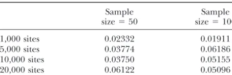
TABLE 2 TABLE 1
Evaluation of asymptotic confidence region Asymptotic and simulated variance of
two-dimensional estimators
Sample Sample
size⫽50 size⫽100 Variance
1,000 sites 0.02332 0.01911 fˆint Tˆ Covariance Correlation
5,000 sites 0.03774 0.06186
Asymptotic
10,000 sites 0.03750 0.05155
1,000 sites 0.03111 0.08806 ⫺0.01804 ⫺0.34
20,000 sites 0.06122 0.05096
5,000 sites 0.006223 0.017612 ⫺0.003608 ⫺0.34
Proportion of simulations where the log-likelihood ratio 10,000 sites 0.003112 0.008806 ⫺0.001804 ⫺0.34
lies outside the two-dimensional asymptotic confidence region 20,000 sites 0.001556 0.004403 ⫺0.000902 ⫺0.34
(log-likelihood ratio ⬎3) is shown. Each value is based on
5000 repetitions with parameter values offrec⫽5,fint⫽0.5, Simulated
andT⫽1. 1,000 sites 0.016781 0.056648 ⫺0.00745 ⫺0.24
5,000 sites 0.005966 0.014237 ⫺0.002720 ⫺0.3
10,000 sites 0.002367 0.007119 ⫺0.001810 ⫺0.44
Power curves:Power analyses were conducted using 20,000 sites 0.001580 0.004182 ⫺0.001040 ⫺0.4
a chi-square test withn ⫺2 d.f. for a sample size ofn
Asymptotic variance is obtained from the estimated
informa-chromosomes to determine the degree of growth that tion matrix as described in the text (Equations 7 and 8). would be required to reject the null hypothesis of con- Results are based on a demographic scenario offrec ⫽ 5.0,
fint⫽0.5, andT⫽1.0 and a sample size of 50 chromosomes.
stant population size using only frequency spectrum
We assumefrecis known and sites are unlinked.
information. For smaller numbers of segregating sites, the degrees of freedom may vary slightly, as frequency categories with expected site counts of less than five are
the null hypothesis with only 5-fold growth (Figure 2a). collapsed. The expected frequency spectrum under the
It is clear that recent rapid growth can be reliably de-null hypothesis is calculated from
tected with frequency spectrum data only with fairly large samples (⬎100 chromosomes), and the most
mod-pi⫽ 1/i
兺
n⫺1j⫽1(1/j)
, 1ⱕ iⱕn ⫺1 (9)
est growth scenarios may be detected only with samples consisting of at least 250 chromosomes when data sets (Ewens1979) by multiplying eachpiby the number of
consist of only 500 (scaled) polymorphic sites. segregating sites. The observed frequency spectrum is
More ancient growth onset:Power to reject the constant obtained by estimating thepi’s from 100,000 replicates
size hypothesis is also dependent upon the time that for each combination offint,frec, andTvalues and then
exponential growth begins, as illustrated in Figure 2b. multinomially sampling from these simulatedpi’s. For
While power is minimal for small sample sizes with each sample size, the number of segregating sites at
growth beginning 10,000 years ago, power increases dra-eachfrecvalue is scaled on the basis of 500 polymorphic
matically with more ancient growth. For example, while sites in a sample size of 20, as described inmodel and
a sample size of 20 with 500 polymorphic sites yields
virtu-methods.
ally no power to detect any magnitude of growth
begin-Recent growth beginning 10,000 years ago: Figure 2a
ning 10,000 years ago, if growth instead began 50,000 shows power curves for the scenario of recent growth
years ago, a sample size of 20 with the same number of beginning at T ⫽ 0.0125 (which, for humans, would
sites would be sufficient to reliably detect 10-fold growth. correspond to 10,000 years ago on the basis of a
genera-Asymptotic properties:We evaluate the distribution of tion time of 20 years andN0of 10,000, roughly
correspond-our maximum-likelihood estimates to determine whether ing to the advent of agricultural society). We consider
asymptotic theory provides an adequate approximation of sample sizes of 10, 20, 50, 100, and 250 chromosomes
the 95% confidence regions and variance associated with with 500 polymorphic sizes (scaled as described above),
our parameter estimates. Table 1 illustrates the proportion which, for a sample size range of 10–250, corresponds to
of maximum-likelihood estimates for which the true a range of 398–859 sites at constant population size
value of the parameters lies outside the asymptotic 95% (frec⫽1) to 390–1137 sites at the most extreme growth
confidence region. Our simulations indicate that for scenario considered (frec⫽ 250). With sample sizes of
large amounts of data, asymptotic theory does provide
ⱕ20, the power to reject the null hypothesis of constant
a good approximation of the 95% confidence region population size never exceeds 0.15, even with 500-fold
for the demographic scenario examined. For smaller growth. With a sample size of 50, power reachesⵑ0.5
amounts of data, the asymptotic approximation appears with 50-fold growth, but barely rises above 0.6 at the
to be conservative, with the true parameter values lying largest magnitude of growth considered. As sample size
within the 95% confidence region inⵑ97–98% of the reaches 100, one can reliably detect 20-fold growth, and
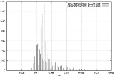
Figure 3.—Distribution of fˆrec
esti-mates. Histograms are based on 5000 sim-ulated data sets wherefrec⫽20 andfintis
fixed at 1. (a) 50 chromosomes, 10,000 sites; (b) 250 chromosomes, 16,244 sites
(T ⫽ 0.0125) and 20,322 sites (T ⫽
0.0625).
the Hausa data set, which consists of 597 sites in a sample maximum-likelihood estimators by examining the distri-bution of the estimates under both two-dimensional and size of 30. For a data set of this size [simulated from
the Hausa maximum-likelihood estimate (MLE)], we three-dimensional models.
Two-dimensional estimators: A recent growth scenario find that asymptotic approximation is especially
conser-vative, rejecting the true parameter values in only 2.04% was examined in which the population size was constant until exponential growth occurred beginning 10,000 of the 5000 simulated data sets.
We also determine the variance and covariance of our years ago. Data sets were simulated withfrecranging from
10- to 320-fold growth, fintfixed at 1, and T⫽ 0.0125
maximum-likelihood estimators in two dimensions by both
asymptotic theory and simulation (Table 2). In this analy- (10,000 years ago based on a generation time of 20 years andN0of 10,000). For this scenario of recent growth,
sis, we assume that Nrec is known and is fivefold ⬎N0
(frec⫽5), whilefintandTare jointly estimated. For this a sample size of at least 250 chromosomes withⵑ16,000
segregating sites is required for 90% of the distribution demographic scenario, asymptotic theory provides a
good approximation for the simulated variance and co- offˆrecto lie within a factor of four of the truefrecvalue for
all magnitudes of growth examined. This is illustrated in variance only when the data set consists of a large
num-ber of segregating sites. Figure 3, which compares thefˆrecdistribution under this
recent growth scenario for sample sizes of 50 and 250 for
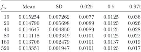
TABLE 3 a factor of 4 of the respective true values with data sets as small as 500 sites in a sample size of 30 (Table 5). If
Distribution ofTˆ
a large data set consisting of 10,000 polymorphic sites in 50 chromosomes were available, 95% of the estimates
frec Mean SD 0.025 0.5 0.975
of all three parameters would lie within a factor of 1.5
10 0.015254 0.007262 0.0077 0.0125 0.0365 of the true parameter values. As would be expected,
20 0.014790 0.005698 0.0089 0.0125 0.0269
estimates of any of the three parameters are improved
40 0.014647 0.004850 0.0089 0.0125 0.0281
by fixing one of the parameters at its true value (data not
80 0.014118 0.003349 0.0101 0.0125 0.0221
shown), indicating that incorporation of prior knowledge
160 0.013706 0.002479 0.0101 0.0137 0.0197
320 0.013331 0.001947 0.0101 0.0125 0.0173 of one of the parameters would be beneficial.
Applications:We apply the maximum-likelihood
meth-Time of expansion isⵑ10,000 years (T⫽0.0125), andfint
od to data obtained from an African Hausa population (A.
is fixed at 1. Simulated data sets consist of 5000 unlinked sites
Di Rienzo, unpublished data) as well as to the
African-in a sample size of 50. TheTˆ grid includes 40 grid points
fromTˆ ⫽0.1(T) toTˆ ⫽4(T). American and European (CEPH) samples of the Seattle SNPs data set (http://pga.gs.washington.edu).
Hausa data:The Hausa data set consisted of the data 20-fold growth. As the magnitude of growth increases,fˆrec of Frisse et al. (2001) in conjunction with additional
becomes biased more severely upward. This result is simi- unlinked locus pairs (A.Di Rienzo, unpublished data), lar to that obtained for growth beginning atT⫽ 0.0625 which resulted in a data set consisting of 30 chromo-(Table 4). somes and 597 polymorphic sites in an African sample, The estimates of T, however, are not subject to the the Hausa of Cameroon. The sites in this data set include upward bias seen infˆrec. Instead, estimates ofTare im- linked polymorphic sites within 50 effectively unlinked
proved as the magnitude of growth increases (Table 3). loci, but in the maximum-likelihood analysis we treat Sample size also has a dramatic effect on the distribution each site as though it provides independent informa-ofTˆ, as illustrated in Figure 4, which compares theTˆ tion. As seen in Table 6,fˆrec⫽3.1,fˆint⫽1, andTˆ ⫽6.1
distribution for sample sizes of 50 and 250. With 5000 for this data set.
sites in a sample size of 50 chromosomes, 95% of Tˆ We perform a 2 goodness-of-fit test on the Hausa
estimates lie within a factor of 3 of the trueTvalue for data set to determine whether the maximum-likelihood 10-fold growth, with 95% of the distribution lying within parameters can be accepted as an explanation of the a factor of 1.5 for 320-fold growth, the most severe Hausa data. However, this test assumes that each site is growth scenario examined. independent, which is not the case for this data set. We explored another growth scenario in which the Because the linkage between sites will affect the 95% onset of growth was more ancient, beginning 50,000 critical value of the2 test statistic, we determine the
years ago. In this case, the quality of the estimators critical value of the test statistic distribution for this improved, and 90% of thefˆrecdistribution was within a data set by coalescent simulation with recombination
factor of four of the truefrecvalue for a sample size of (Hudson1983, 2002). We simulate 5000 data sets, each
50 with 5000 sites (as opposed to a sample size of 250 and consisting of 30 chromosomes and 50 unlinked loci.
ⵑ16,000 sites under the more recent growth scenario). The input parameters for the simulation included Watt-Figure 3 reveals the improvement in thefˆrec estimator erson’s estimate of (estimated to be 0.0012/bp), the
with the more ancient time of growth onset. As in the recombination rate (estimated to be 5.99⫻10⫺4/bp), recent growth scenario, increasing the degree of growth the average locus length (10,286 bp), and a gene-conver-both increased the bias and widened the quantiles of sion to crossing-over ratio of 2. Polymorphic sites within the fˆrec distribution (Table 4). The Testimates under the middle 8000 bp were ignored to mimic the locus
the more ancient growth scenario were also improved pair data (Frisse et al. 2001). Because the ancestral/ over the analogous recent growth estimates, with 95% derived status of each allele was not considered, each of theTˆ distribution within a factor of two of the true simulated frequency spectrum was folded at frequency
T value for all magnitudes of growth examined with 0.5 prior to performing the2 goodness-of-fit test. On
data sets as small as a sample size of 50 with 1000 sites. the basis of these simulations, we found the 95% critical
Three-dimensional estimators: We consider a three- value of the 2 test statistic to be 39.39, as opposed
dimensional model of a constant-sized population that to a critical value of 23.68 (14 d.f.) if all sites were experienced an instantaneous decrease to 0.05 times independent. The2goodness-of-fit test statistic for the
its initial size 100,000 years in the past, followed by Hausa data set under its maximum-likelihood estimate exponential growth until the present to a final size of offˆrec⫽3.1,fˆint⫽1, andTˆ ⫽6.1 is 26.30 (P⫽0.304),
Figure4.—Distribution ofTˆ
estimates. Histograms are
based on 5000 simulated data
sets with parametersfrec ⫽20,
fint ⫽ 1 (fixed), T ⫽ 0.0125,
each consisting of 10,000 poly-morphic sites in 50 chromo-somes or 16,244 polymorphic sites in 250 chromosomes.
We also considered the equilibrium model of constant simulation. Additional analyses incorporating more of the SNPs are described in the discussion. The fre-population size for this data set and obtained a2
good-ness-of-fit test statistic of 29.24 (P⫽0.204). On the basis quency spectrum of nonsynonymous SNPs has been shown to differ from that of synonymous SNPs (Cargill
of an analysis of 10 locus pairs (a subset of the 50 locus
pairs examined here), Frisse et al. (2001) also con- et al.1999;Fayet al.2001;WoodingandRogers2002), so we also removed all SNPs that result in an amino-cluded that the Hausa data are consistent with the
equi-librium model. acid coding change to minimize the inclusion of those SNPs subject to nonneutral evolutionary processes. This
Seattle SNPs:We also examined both the
African-Amer-ican and the European samples of the Seattle SNPs data, resulted in a final data set of 5892 SNPs for the African-American data set and 4211 SNPs for the European data which are located at the University of Washington-Fred
Hutchinson Cancer Research Center (UW-FHCRC) Varia- set. We applied our maximum-likelihood method to these data sets, treating all SNPs as unlinked, and found tion Discovery Resource (http://pga.gs.washington.edu).
These data sets consist of 12,587 and 7712 total SNPs that the three-dimensional maximum-likelihood esti-mates offrec,fint, andTarefˆrec⫽ 1.9,fˆint ⫽1, and Tˆ ⫽
across 138 loci in the African-American and European
samples, respectively. We considered only those SNPs 0.27 for the African-American data set andfˆrec⫽2,fˆint⫽
0.15, andTˆ ⫽0.0375 for the European data set (Table that were sequenced in the entire panel of 48
(African-American) or 46 (European) chromosomes to facilitate 6). These estimates suggest a scenario of very slow growth over a long period of time with no bottleneck evaluation of confidence regions and goodness-of-fit by
for the African-Americans and a fairly recent population bottleneck withⵑ13-fold recovery for the Europeans.
TABLE 4
Distribution offˆrec/frec TABLE 5
Distribution of three-dimensional MLEs
frec Mean SD 0.05 0.5 0.95
10 1.0674 0.2926 0.7 1.0 1.6 Mean SD 0.05 0.5 0.95
20 1.0925 0.3862 0.7 1.0 1.7
40 1.1629 0.5722 0.6 1.0 2.2 fˆrec 6.017479 4.233278 1.5 5 15
80 1.2980 0.8200 0.5 1.0 3.3 fˆint 0.056695 0.042797 0.01 0.045 0.14
160 1.3906 1.0092 0.4 1.0 3.9 Tˆ 0.112958 0.038210 0.055 0.115 0.175
320 1.5072 1.1824 0.3 1.0 3.9
Simulated data sets consist of 500 sites in a sample size of
30 chromosomes, wherefrec⫽5.0,fint⫽0.05, andT⫽0.125.
Time of expansion isⵑ50,000 years (T⫽0.0625), andfint
is fixed at 1. Simulated data sets consist of 5000 unlinked sites The three-dimensional grid includes fˆrec values from 0.5 to
14.5 (at 0.5 intervals),fˆintvalues from 0.01 to 0.15 (at 0.005
in a sample size of 50. The fˆrecgrid includes 40 grid points
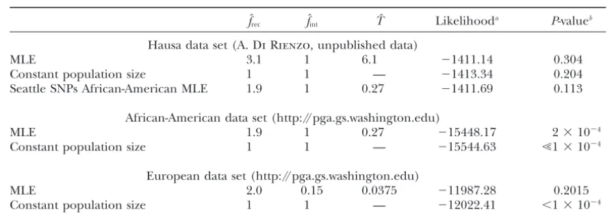
TABLE 6
Hausa and Seattle SNPs analysis
fˆrec fˆint Tˆ Likelihooda P-valueb
Hausa data set (A.Di Rienzo, unpublished data)
MLE 3.1 1 6.1 ⫺1411.14 0.304
Constant population size 1 1 — ⫺1413.34 0.204
Seattle SNPs African-American MLE 1.9 1 0.27 ⫺1411.69 0.113
African-American data set (http://pga.gs.washington.edu)
MLE 1.9 1 0.27 ⫺15448.17 2⫻10⫺4
Constant population size 1 1 — ⫺15544.63 Ⰶ1⫻10⫺4
European data set (http://pga.gs.washington.edu)
MLE 2.0 0.15 0.0375 ⫺11987.28 0.2015
Constant population size 1 1 — ⫺12022.41 ⬍1⫻10⫺4
aNote that this is not true likelihood since the segregating sites are not entirely unlinked.
bP-values are calculated from a2goodness-of-fit test where the distribution of the2test statistic is simulated
for each data set, accounting for linkage as described in the text.
To determine whether the demographic model we nation of the African-American data set, although the fit is better than that predicted by the constant popula-consider is compatible with the Seattle SNPs data, we
simulate the distribution of the goodness-of-fit test statis- tion size model (2⫽268.66;PⰆ1⫻10⫺4). Figure 5
provides a visual comparison of the observed Seattle tic for this data set as described for the Hausa data set.
For these simulations, each data set consisted of 48 chro- SNPs frequency spectrum to the frequency spectra pre-dicted by both the maximum-likelihood parameters and mosomes and 138 loci. The input parameters were that
of the Hausa data set, except substituting the average constant population size parameters, indicating that the lack of fit of the maximum-likelihood parameters does length of a Seattle SNPs locus. In this case, each locus
was simulated, fixing the number of segregating sites not seem to be confined to any particular nonsingleton frequency class. However, our demographic model with to be the average number of segregating sites per locus
in the African-American or European Seattle SNPs data the maximum-likelihood parameters appears to provide a better fit to the data than the equilibrium model, set, so each simulated data set contained the same total
number of segregating sites as our observed Seattle SNPs particularly in the singleton class. In addition, we note that a2goodness-of-fit test shows that the Hausa data
African-American or European data set. Because the
Seattle SNPs data sets do not specify the ancestral/de- are compatible with frec ⫽ 1.9, fint⫽ 1, and T⫽ 0.27,
the estimates obtained from the Seattle SNPs African-rived status of each allele, each simulated frequency
spectrum is again folded. The 95% critical values of American data set (2⫽33.46;P⫽0.113).
Because the sites in the Hausa and Seattle SNPs data the distribution were found to be 48.68 (African) and
137.36 (European) as opposed to 35.17 (23 d.f.) and sets are not entirely unlinked, asymptotic approxima-tion of confidence intervals is not appropriate. We simu-33.92 (22 d.f.) if all sites were unlinked.
Using these simulated critical values, a2 goodness- lated 10,000 data sets as described above for both the
Hausa and Seattle SNPs data sets, using their respective of-fit test indicates that the maximum-likelihood
param-eters produce an expected frequency spectrum that is maximum-likelihood estimates for input parameters, and applied the maximum-likelihood method to the not significantly different from the observed Seattle
SNPs European data (2⫽122.98;P⫽0.2015). There- folded frequency spectrum of each simulated data set.
For the Hausa and Seattle SNPs African-American data fore, we can accept our simple bottleneck model as a
reasonable explanation for this data set. The same test sets, we estimated bothfrecandT, fixingfintat 1, which
was the maximum-likelihood estimate for both data sets. indicates that a constant population size model is not
compatible with the European data (2⫽207.286;P⬍ All three parameters were estimated for the data sets
simulated from the Seattle SNPs European parameters. 1⫻ 10⫺4).
However, the 2 goodness-of-fit test on the African- The ratio of the log-likelihood at the
maximum-likeli-hood parameters to the log-likelimaximum-likeli-hood at the parameters American data set reveals that the frequency spectrum
predicted by the maximum-likelihood estimates offrec, from which the data set was simulated could then be
calculated. From the log-likelihood ratio distribution,
fint, and Tis significantly different from the empirical
Seattle SNPs African-American frequency spectrum we determined the 95% critical value to be 3.86 for the Hausa data set and 4.85 for the Seattle SNPs African-(2⫽86.64;P⫽2⫻10⫺4); therefore, our simple
parameters corresponding to the Seat-tle SNPs maximum-likelihood estimate (frec⫽1.9,fint⫽1, andT⫽0.27) and
constant population size are shown. The number of SNPs at a sample
fre-quency ofiis equal to the total number
of SNPs (5892) timespi(folded). For
constant population size, pi’s are
ob-tained from Equation 9, and, for the
maximum-likelihood parameters, pi’s
are obtained from simulation as de-scribed in the text.
value of 3.0 for two-dimensional maximum-likelihood segregating sites (15,838–17,140 segregating sites de-pending upon the true frecvalue) are required for the
estimates. The 95% critical value of 9.1 was found for
the European data set as compared to the asymptotic fˆrecdistribution to have 95% critical values that fall within
a factor of four of the truefrecvalue if growth began as
critical value of 3.9 for three-dimension estimation.
Us-ing the critical values from simulation, we can easily recently as 10,000 years ago (T⫽0.0125). Unless large sample sizes and many unlinked sites are surveyed, the reject the constant-size population model for the Seattle
SNPs African-American and European data sets since frequency spectrum alone provides little information about the magnitude of growth that has occurred rela-the log likelihood ratios are 96 and 35, respectively
(Table 6). tively recently. Asfrecincreases, the frequency spectrum
Figure 6a provides a visual representation of the 95, becomes more distinct from what would be expected 99, and 99.9% confidence regions of the Hausa data under a constant size scenario. However, with increas-set obtained by including all parameter values for which ingly extreme recent growth, the frequency spectrum the log-likelihood ratio isⱕ3.86, 6.38, and 10.08, respec- becomes less distinguishable from that of other severe tively. Likewise, Figure 7 illustrates the analogous con- growth scenarios, and it becomes more difficult to esti-fidence regions for the Seattle SNPs African-American mate thefrecparameter with frequency spectrum
infor-(Figure 7a) and European infor-(Figure 7b) data sets. mation alone.
While it is difficult to accurately estimatefrecfor
scenar-ios of recent growth, T can be estimated with more
DISCUSSION modest amounts of data. The distribution ofTˆhas 95%
critical values that fall within a factor of four of the true Our power analyses on models with exponential
T value for sample sizes as small as 50 chromosomes growth beginning 10,000 years ago illustrate that the
and 5000 sites, as compared to a sample size of 250 and frequency spectrum does not provide sufficient
informa-15,838–17,140 sites required to estimatefrecto the same
tion to reject the null hypothesis of constant population
accuracy. Additionally, Tˆ is not subject to the upward size when either small sample sizes (⬍50 chromosomes)
bias seen infˆrecand estimates ofTactually improve with
or small numbers of unlinked sites (⬍1000) are
avail-increasing frec. Estimates of bothfrecand Timprove as
able. This result should serve as a cautionary note to
the onset of growth becomes more ancient. This obser-researchers interested in demographic models involving
vation is consistent with our observation that power to expansion as recent as 10,000 years ago. Prior
knowl-reject the null hypothesis of constant population size edge of the model of interest should also be considered
with frequency spectrum data increases with scenarios when determining whether the frequency spectrum
re-of more ancient growth (Figure 2b). tains the requisite information for demographic inference,
Simultaneous estimation of all three parameters re-as the power to detect departures from constant size
in-sults in estimator distributions where 90% of the esti-creases with both the extent of growth (Figure 2, a and
mates lie within a factor of four of the true parameter b) and the time since the onset of growth (Figure 2b).
values with data sets as small as 500 segregating sites in Application of the maximum-likelihood method on
a sample size of 30 for a model where the population recent growth scenarios reveals that data sets consisting
Figure 7.—Seattle SNPs confidence regions. (a)
African-Figure6.—Hausa confidence region. The third dimension,
American data set, with MLE indicated by the arrow (fˆrec⫽
fint, is fixed at 1. (a) Maximum-likelihood estimate (MLE) is
1.9,Tˆ ⫽0.27). The third dimension,fint, is fixed at the MLE
indicated by the arrow (fˆrec ⫽3.1, Tˆ ⫽6.1). (b) Focus on
offˆint⫽1. (b) European data set, with MLE indicated by the
recent growth times with expandedfrecrange. The leftmost,
arrow (fˆint⫽0.15,Tˆ ⫽0.0375). The third dimension (frec) is
middle, and rightmost contours represent the 95, 99, and
fixed at the MLE offˆrec ⫽2.0. The innermost, middle, and
99.9% confidence intervals (3.86, 6.38, and 10.08
log-likeli-outermost contours surrounding the MLE represent the 95, hood units, respectively).
99, and 99.9% confidence regions, respectively.
ago and the present population is only five times the
Evaluation of the asymptotic properties of our maxi-initial population size. These estimates benefit from
mum-likelihood estimators indicates that asymptotic both a more ancient time of growth onset and a modest
theory provides a reasonable approximation of the con-magnitude of growth that is not subject to the upward
fidence intervals associated with the estimators. As we bias seen in more severe growth scenarios. The ability
illustrate with the Hausa and Seattle SNPs data sets, it of the frequency spectrum alone to elucidate the time
is also possible to construct these confidence intervals and magnitude of population size change events is,
around a maximum-likelihood estimate through simula-therefore, greatly dependent upon the underlying
de-tion. By simulating data sets that closely match the prop-mographic model. While ancient deprop-mographic events
erties of the observed data set, one can estimate the may be inferred relatively accurately from contemporary
critical value of this log-likelihood ratio distribution and frequency spectrum patterns, more recent and severe
construct corresponding confidence regions. This pro-episodes of growth are problematic for this method and
cedure is particularly relevant when asymptotic approxi-require exceedingly large amounts of unlinked data.
mation is not appropriate, such as when the segregating For these recent growth scenarios, it is possible that
sites in a data set are not unlinked. more informative estimates could be obtained by using
We apply the maximum-likelihood method to both a method that uses linked polymorphic sites and
consid-the African Hausa data set and consid-the African-American ers additional aspects of the data such as levels of linkage
account the linkage between sites. The African-American population sampled for the Seattle SNPs data set may also be subject to population In the Seattle SNPs African-American data set, the
simulated 95% confidence interval clearly allows for structure and admixture, which could affect the fre-quency spectrum and confound our inference about rejection of the constant population size model, since
the log-likelihood of observing the data is almost 100 demographic history (PtakandPrzeworski2002). To determine the effect of European admixture on maxi-units less with the constant size parameters than with
the estimated parameters. The maximum-likelihood es- mum-likelihood estimates obtained from an African data set, we randomly combined 6 Italian chromosomes (A. timates offˆrec⫽1.9,fˆint⫽1, andTˆ ⫽0.27 based on the
Seattle SNPs African-American data correspond to a Di Rienzo, unpublished data) with the 30 Hausa chro-mosomes at each of the 50 locus pairs of the Hausa data slow, ancient growth scenario where growth began
⬎200,000 years ago to a present size of approximately set, which resulted in a total data set of 657 polymorphic sites in 36 chromosomes. This representsⵑ17% Euro-two times the initial population size.
The simulated 95% confidence region around the pean admixture, which is consistent with admixture esti-mates obtained from African-American populations Seattle SNPs African-American maximum-likelihood
es-timates, shown in Figure 7a, includes only a very narrow (Parraet al.1998). Admixture of this proportion had virtually no effect on the maximum-likelihood estimates range offrecvalues within 1.6–2.5. However, the
confi-dence region includes a wide range ofTvalues ranging or confidence intervals based on the original Hausa data set (data not shown). Regardless, that does not eliminate from as recent as 80,000 years ago (T⫽0.1) to the most
ancient time examined, 800,000 years ago (T ⫽ 1), the possibility that either the true population structure could involve admixture in different proportions or ad-assuming a generation time of 20 years and an N0 of
10,000. Even with the most recent compatibleTvalue, mixture in a larger data set such as the Seattle SNPs would produce a more prominent effect. The frequency it is not surprising that this data set allows for rejection
of the constant size hypothesis with an estimate of only spectrum of the Seattle SNPs data set is certainly not consistent with an equilibrium model of constant popu-twofold growth. Our power analyses show that a data
set consisting of 50 chromosomes has a power of 0.9 lation size, although the degree of growth predicted is less than that of some previous reports based on African to reject the constant size hypothesis with only 1000
unlinked sites for twofold growth beginning 100,000 populations (Aris-BrosouandExcoffier1996; Pritch-ardet al.1999). However, our estimate of twofold growth years ago. While the Seattle SNPs data set does not
consist of entirely unlinked sites, our analysis included beginning as recently as 80,000 years ago is consistent with a recent study based on the frequency spectrum
⬎5000 polymorphic sites across 138 loci, which should
allow for comparable power. in an African-American population (Marthet al.2004). The maximum-likelihood parameters estimated from Despite the compact confidence region (Figure 7a),
visually reasonable fit of the frequency spectrum under this data set are consistent with the Hausa data set, which contains noncoding loci that are less likely to be the maximum-likelihood parameters to the observed
data (Figure 5), and compatibility with the Hausa data subject to confounding factors such as selection. How-ever, this analysis does not preclude population struc-set, a 2 goodness-of-fit test indicates that our simple
three-dimensional demographic model with the maxi- ture within Africa as a potential influence on the maxi-mum-likelihood estimates of the Hausa data set. The mum-likelihood estimates obtained from the Seattle
SNPs African-American data set is incompatible with the maximum-likelihood estimates from the Hausa data set (fˆrec⫽3.1,fˆint⫽1, andTˆ⫽6.1) correspond to a scenario
Seattle SNPs data (P⫽ 2 ⫻ 10⫺4), even when linkage
is taken into account. The visual comparison between of slow, ancient threefold growth, beginning several mil-lion years ago. However, the confidence region associ-the observed and maximum-likelihood frequency
spec-tra in Figure 5 seems to indicate that the number of ated with this data set (Figure 6a) is consistent with a wide range of growth scenarios, including both the singletons expected under the maximum-likelihood
pa-rameters is very close to the observed value, and there- demographic history estimated from the Seattle SNPs data set (fˆrec⫽1.9,fˆint⫽1, andTˆ ⫽ 0.27) andfrec⫽ 1,
fore the incompatibility must be due to some
combina-tion of the other frequency categories. The loci in the which corresponds to constant population size. Addi-tionally, Figure 6b provides a close-up view of the accep-Seattle SNPs data set were chosen because of their role
in inflammatory pathways and may reflect the action of tance region of Figure 6a, considering only more recent values ofTwhere the onset of growth occurs no more evolutionary forces other than population size changes.
clear that our confidence regions on this data set do confounding factors to consider when attempting to infer demographic history based on frequency spectrum not exclude scenarios of 20-fold or more growth,
pro-vided that the time of onset is correspondingly more information, including population structure (past or present) and selection. An additional complication that recent. For example, if we believe that the Hausa
popula-tion has undergone growth⬎5-fold, then our analysis is not considered by these analyses is ascertainment bias and genotyping error. It has been shown that ascertain-indicates that the growth must have begun no earlier
thanT⫽0.045 (36,000 years ago ifN0is 10,000 assuming ment bias can lead to large errors in
maximum-likeli-hood-based demographic inference (Kuhner et al.
a generation time of 20 years). Growth of that
magni-tude or larger is rejected at the 1% level (Figure 6b) 2000; Wakeley et al. 2001). Polanski and Kimmel
(2003) have also shown that exclusion or misclassifica-for values ofT ⬎0.045 and ⬍3 (ⵑ36,000–2.4 million
years ago). tion of low-frequency SNPs can result in estimated growth rates that are significantly lower than the true Our analysis of the Seattle SNPs European data set
reveals an estimated demographic history offˆrec⫽2.0, value. Note, however, that the sites represented in the
Di Rienzo and Seattle SNPs data sets were chosen
with-fˆint ⫽ 0.15, and Tˆ ⫽ 0.0375, which corresponds to an
85% reduction in population size atT⫽0.0375 (30,000 out prior indication of polymorphism status. Therefore, the analyses on these data sets would not be influenced years ago assumingN0⫽10,000 and a 20-year generation
time) and thenⵑ13-fold exponential growth to a cur- by ascertainment bias due to using a discovery sample for SNP identification. However, we cannot exclude the rent population size of twice the ancestral size. In
con-structing our data set, we exclude all SNPs that are possibility that genotyping errors have biased our infer-ences.
not successfully typed in every chromosome to facilitate
construction of appropriate confidence regions and esti- Conclusions: Analysis of this maximum-likelihood method indicates that demographic inferences can be mation of2 critical values through simulation.
How-ever, we note that if all SNPs that were typed in at least drawn from frequency spectrum data when sufficient amounts of data are available. Asymptotic theory or sim-half of the sampled chromosomes (7410 SNPs) were
included in this analysis, we get only a slightly different ulation can be used to determine the variance and covar-iance associated with these estimators to determine estimate (fˆrec⫽1.25,fˆint⫽0.2, andTˆ ⫽0.05) that differs
by ⬍2 log-likelihood units from our maximum-likeli- whether the maximum-likelihood estimates would be meaningful for a particular demographic model and hood estimate based on the filtered data (⫺20,668.96vs.
⫺20,670.93 when all SNPs are included). Since the 95% amount of data that may be available. However, our results show that very large amounts of data may be confidence region includes all parameter values within
9.1 log-likelihood units from the maximum, it is not required to obtain practical confidence regions, particu-larly in models involving recent growth. For growth be-likely that this filtering of the data would result in a
significant shift in our acceptance region. ginning as recently as 10,000 years ago, the power to reject the hypothesis of constant population size is very A2goodness-of-fit test indicates that frequency
spec-trum produced by the estimated parameters (fˆrec⫽2.0, low with sample sizes of⬍20 chromosomes. To make
accurate inferences under this type of recent-growth
fˆint⫽ 0.15, and Tˆ ⫽ 0.0375) is a reasonable match to
the observed Seattle SNPs European frequency spec- model using the frequency spectrum alone, both large samples (⬎100 chromosomes) and a large number of trum with aP-value of 0.2015. The constant size model
is both rejected by the goodness-of-fit test and excluded unlinked sites (⬎5000 sites) are required, although esti-mators improve as the time of onset of growth becomes by the simulated likelihood-ratio confidence region for
this data set (Table 6, Figure 7b). These results implicate more ancient. In scenarios of extreme growth, there is also a severe bias infˆrec, even with large amounts of data.
a bottlenecked history for this European data set, which
is consistent with previous studies (Marthet al. 2003, However,Tcan be estimated with more modest amounts of data, and Tˆ is not subject to the bias seen in fˆrec,
2004) and the “Out of Africa” model for human
popula-tion history (Harpendinget al.1998). Since the Seattle indicating that one may obtain reasonable estimates of the time of population size-change events, even if the SNPs European data set is composed of the same coding
loci as the Seattle SNPs African-American data set, it magnitude is biased. This maximum-likelihood method incorporates all available information contained in un-seems reasonable that the lack of agreement between
the frequency spectrum predicted by the maximum- linked polymorphic sites, and parameter estimation methods based on summaries of the frequency spectrum likelihood parameters and the observed
African-Ameri-can frequency spectrum is more likely to be due to require even larger amounts of data to be equally as informative. Therefore, for scenarios where the entire population structure than to the presence of slightly
deleterious variants in the data set. Of course, the good frequency spectrum of modest data sets does not pro-vide an adequate amount of information, it may be fit of the European maximum-likelihood parameters
does not preclude the possibility of population structure necessary to incorporate additional aspects of linked data to improve estimates of demographic parameters. or selection within the European data set as well.
cent. Genetics149:429–434. ⬎36,000 and⬍2.4 million years ago on the basis of this
Kuhner, M. K., P. Beerli, J. YamatoandJ. Felsenstein, 2000
Use-data set. The Seattle SNPs African-American Use-data set fulness of single nucleotide polymorphism data for estimating
population parameters. Genetics156:439–447.
also supports a model of growth, although a
goodness-Marth, G., G. Schuler, R. Yeh, R. Davenport, R. Agarwalaet al.,
of-fit test indicates that the best-fit model of ancient,
2003 Sequence variations in the public human genome data
slow growth is not sufficient to explain the observed reflect a bottlenecked population history. Proc. Natl. Acad. Sci. frequency spectrum. Maximum-likelihood analysis of the USA100(1): 376–381.
Marth, G., E. Czabarka, J. MurvaiandS. T. Sherry, 2004 The
Seattle SNPs European data set reveals that the
best-allele frequency spectrum in genome-wide human variation data
fit model is one of a population bottleneck occurring reveals signals of differential demographic history in three large
ⵑ30,000 years ago, reducing the population to 15% of world populations. Genetics166:351–372.
Nielsen, R., 1999 Estimation of population parameters and
recom-the ancestral size, followed by 13-fold growth to a
cur-bination rates from single nucleotide polymorphisms. Genetics
rent population size that is twice the ancestral size. 154:931–942.
Parra, E. J., A. Marcini, J. Akey, J. Martinson, M. A. Batzeret al., We thank A. Di Rienzo for access to the Hausa data set prior to
1998 Estimating African American admixture proportions by publication. Construction of the Hausa data set was supported by
use of population-specific alleles. Am. J. Hum. Genet.63:1839– National Institutes of Health (NIH) grant HG-02098. A. Adams was
1851. supported by NIH/National Institute of General Medical Sciences
Pluzhnikov, A., A. Di RienzoandR. R. Hudson, 2002 Inferences grant 5 T32 GM07197. about human demography based on multilocus analyses of
non-coding sequences. Genetics161:1209–1218.
Polanski, A., andM. Kimmel, 2003 New explicit expressions for relative frequencies of single-nucleotide polymorphisms with ap-LITERATURE CITED
plication to statistical inference on population growth. Genetics
165:427–436. Aris-Brosou, S., andL. Excoffier, 1996 The impact of population
expansion and mutation rate heterogeneity on DNA sequence Pritchard, J. K., M. T. Seielstad, A. Perez-Lezaun and M. W. polymorphism. Mol. Biol. Evol.13(3): 494–504. Feldman, 1999 Population growth of human Y chromosomes: Beerli, P., andJ. Felsenstein, 2001 Maximum likelihood estima- a study of Y chromosome microsatellites. Mol. Biol. Evol.16(12):
tion of a migration matrix and effective population sizes in n 1791–1798.
subpopulations by using a coalescent approach. Proc. Natl. Acad. Ptak, S. E., andM. Przeworski, 2002 Evidence for population Sci. USA98:4563–4568. growth in humans is confounded by fine-scale population struc-Cargill, M., D. Altshuler, J. Ireland, P. Sklar, K. Ardlieet al., ture. Trends Genet.18:559–563.
1999 Characterization of single-nucleotide polymorphisms in Tajima, F., 1989 Statistical method for testing the neutral mutation coding regions of human genes. Nat. Genet.22:231–238. hypothesis by DNA polymorphism. Genetics123:585–595. Ewens, W. J., 1979 Mathematical Population Genetics. Springer-Verlag, Wakeley, J., R. Nielsen, S. N. Liu-Cordero andK. Ardlie, 2001
New York. The discovery of single-nucleotide polymorphisms—and infer-Fay, J. C., J. Wyckoff and C.-I Wu, 2001 Positive and negative ences about human demographic history. Am. J. Hum. Genet.
selection on the human genome. Genetics158:1227–1234. 69:1332–1347.
Frisse, L., R. R. Hudson, A. Bartoszewicz, J. D. Wall, J. Donfack Wall, J. D., andM. Przeworski, 2000 When did the human
popula-et al., 2001 Gene conversion and different population histories tion size start increasing? Genetics155:1865–1874.
may explain the contrast between polymorphism and linkage Weiss, G., andA. Von Haeseler, 1998 Inference of population disequilibrium levels. Am. J. Hum. Genet.69:831–843. history using a likelihood approach. Genetics149:1539–1546. Griffiths, R. C., andS. Tavare´, 1998 The age of a mutation in Wooding, S., andA. Rogers, 2002 The matrix coalescent and an
the general coalescent tree. Stoch. Models14:273–295. application to human single-nucleotide polymorphisms. Genetics Harpending, H. C., M. A.Batzer, M.Gurven, L. B.Jorde, A. R. 161:1641–1650.
Rogerset al., 1998 Genetic traces of ancient demography. Proc.