DOI: 10.1534/genetics.107.071910
Postprocessing of Genealogical Trees
Loukia Meligkotsidou
1and Paul Fearnhead
Department of Mathematics and Statistics, Lancaster University, Lancaster, LA1 4YF, United Kingdom Manuscript received February 9, 2007
Accepted for publication May 17, 2007
ABSTRACT
We consider inference for demographic models and parameters based upon postprocessing the output of an MCMC method that generates samples of genealogical trees (from the posterior distribution for a specific prior distribution of the genealogy). This approach has the advantage of taking account of the uncertainty in the inference for the tree when making inferences about the demographic model and can be computationally efficient in terms of reanalyzing data under a wide variety of models. We consider a (simulation-consistent) estimate of the likelihood for variable population size models, which uses impor-tance sampling, and propose two new approximate likelihoods, one for migration models and one for con-tinuous spatial models.
T
HERE are two common approaches to analyzing population genetic data. The first approach in-volves (i) inferring a genealogical or phylogenetic tree for the data and (ii) making inferences about demo-graphic or other parameters conditional on this tree. Examples of this include inference of the demography (Underhillet al. 2001), nested clade analysis (Templetonet al. 1987), and phylogeographic and spatial analysis (Emersonand Hewitt2005; French et al. 2005). Of-ten this approach is applied informally, with the qualita-tive features of the inferred tree being used to suggest plausible demographic histories for the sample (e.g., Shen
et al. 2000).
The second approach involves joint inference of the genealogical tree and the parameters. In many cases the genealogical tree is a nuisance parameter, and calcula-tion of the likelihood for the parameters involves inte-grating out the unknown tree, for example, in inference about various demographic models under a coalescent prior, including variable population sizes (Griffiths and Tavare´1994a; Kuhneret al. 1998; Drummondet al. 2005) and population structure (Bahloand Griffiths 1998; Beerli and Felsenstein 1999), inference for selection (Coop and Griffiths 2004), dispersal of a population (Brookset al. 2007), and inference for re-combination rates (Griffiths and Marjoram 1996; Kuhneret al. 2000; Fearnheadand Donnelly2002). (In the latter case the genealogical information is con-tained in a graph and not in a tree.)
The advantage of the second approach is that, assum-ing the model for the genealogical tree is reasonable,
the uncertainty in this genealogy is correctly incorpo-rated into the inference about the parameters of inter-est. This is particularly important for data where there is considerable uncertainty in the genealogy (which is common for many data sets). The first approach of conditioning on a single estimate of the genealogy can sometimes lead to biases in estimates and, more gen-erally, to underestimates of the uncertainty in the pa-rameters. These problems often mean that analysis conditional on the tree is often used primarily to test hypotheses (Templetonet al. 1987; Frenchet al. 2005), rather than for estimating parameters of appropriate models.
However, implementing the second approach is con-siderably more challenging and generally requires the use of modern computationally intensive statistical meth-ods (Stephensand Donnelly2000). In particular, this often requires the development of customized programs to analyze the data under the specific model or models of interest, and the application of this approach can be limited by the availability of suitable software.
In this article we consider a new approach, which lies between these two approaches. The basic idea is (i) to perform inference for the genealogical/phylogenetic tree using a suitable Bayesian approach, obtaining a sample of trees from the posterior and (ii) to perform inference on the parameters of interest using this sam-ple of trees. The idea is that by using a samsam-ple of trees in an appropriate way we can still take account of the uncertainty within the inference for the tree, but that this approach will be less computationally intensive and more widely applicable than the second approach above. We consider inference under three different demo-graphic models: (a) variable population size, (b) migra-tion between discrete subpopulamigra-tions, and (c) continuous 1Corresponding author: Department of Mathematics and Statistics,
Lancaster University, Lancaster, LA1 4YF, United Kingdom. E-mail: [email protected]
spatial structure. For model a we present a simple importance-sampling approach that can reweight a sam-ple of trees so that the resulting weighted samsam-ple ap-proximates the posterior distribution of the genealogy under any variable population size model. For models b and c we propose approximate-likelihood functions based on specifying a probability model for the pop-ulation or on spatial information of the sample given the genealogy.
Our aim is to evaluate the potential for this approach of postprocessing a sample of genealogical trees. As such we focus on the specific case of inference for a non-recombining DNA region with infinite-sites data and known topology. The advantage of focusing on this spe-cial case is that there exists an algorithm for simulating directly from the posterior distribution of the coales-cence times of the tree, under a specific prior (see methods). Thus we can focus on the computational and statistical efficiency of the postprocessing methods, without any need to take into account the possible effects of any inaccuracies in the method for generating the sample of trees. However, the ideas of postprocess-ing can be applied to the output of any MCMC or other approach for generating samples of trees from a known posterior distribution and thus are not restricted to the assumptions of infinite-sites data or known topology.
METHODS
Infinite-sites data and phylogenetic prior: We focus on analyzing data frommchromosomes sampled from a population. We assume we have infinite-sites data from a nonrecombining region of the genome and that the topology of the genealogy is known. The infinite-sites data mean that we will know the number of mutations that have occurred on each branch of the genealogy. Our mutation model is that (for our chosen scaling of time) these mutations occur at a constant rateu/2 along each branch of the genealogy.
We assume some labeling of the nodes in the gene-alogy and denote by t ¼(t1,. . ., tm1) the coalescent
times for these nodes. We take the usual convention of the current time being time 0 and time being measured backward into the past. We also introduce the notation
t9 ¼ (t91,. . ., tm9 1) to denote the ordered coalescent
times (sot91,t92,. . .,tm9 1). In the genealogy there are
2(m1) branches. The branch lengths are denoted by
b ¼(b1,. . .,b2(m1)), and sequence data can be
sum-marized by the number of mutations on each branch:
n¼(n1,. . .,n2(m1)). The branch lengths,b, are a linear
function of the coalescent times,t; and to emphasize their interdependence we writeb(t) andbi(t). The like-lihood of the data,n, can be written as
pðnjt;uÞ ¼ Y 2ðm1Þ
i¼1
u
2 ni
biðtÞni expfbiðtÞu=2g: ð1Þ
Now we use the pure birth process prior of Rannala and Yang (1996) for the coalescent times, which as-sumes that the length of each branch has an exponen-tial distribution with ratef,
p1ðtjfÞ}Y m1 i¼1
ðm11iÞfexpfðm11iÞfðt9it9i1Þg:
ð2Þ
Under this prior the posterior distribution fort(given
fandu) is
pðtjn;u;fÞ}fm1 Y 2ðm1Þ
i¼1
u
2 ni
biðtÞniexpfðf1u=2ÞbiðtÞg:
ð3Þ
Note that setting f ¼ 0 produces a posterior that is proportional to the likelihood function.
By introducing new variabless¼(s1,. . .,sm1), which
satisfysi¼(f1u/2)ti, we obtain
pðsjn;u;fÞ} f
f1u=2
m12ðYm1Þ
i¼1
u=2
f1u=2
ni
3ðbiðsÞÞniexpðbiðsÞÞ; ð4Þ
where by the linear relationship between branch lengths and coalescent timesbi(s)¼(f1u/2)bi(t). Fearnhead and Meligkotsidou (2004) show how to draw inde-pendent and identically distributed (i.i.d.) samples from this density and hence (through rescaling) from the pos-terior (3). Furthermore this gives that the likelihood for
fis proportional to
f f1u=2
m1 u=2
f1u=2
n
; ð5Þ
wherenis the total number of mutations.
Variable population size:Consider a panmictic pop-ulation of current effective poppop-ulation sizeN chromo-somes, with time measured in units of N generations, and let the effective population size at timetin the past beN/l(t). The distribution for the coalescence times for a random sample ofmchromosomes from such a population (Griffithsand Tavare´1994a) is
p2ðtjlðÞÞ ¼Y m1 i¼1
m11i
2
lðti9Þ
3exp m11i 2
ðLðti9Þ Lðti91ÞÞ
;
ð6Þ
whereLðsÞ ¼Ð0slðuÞdu, and remember that theti’s are9 defined as ordered coalescent times.
in calculating the marginal likelihoodp(njl(),u). The former allows us to perform inference for a given de-mographic model, and the latter is required for choos-ing between different demographic models.
Both of these can be achieved through an algorithm that generates samples of the coalescent times from (3) and then reweights these samples. For example,
pðnjlðÞ;uÞ ¼
ð
p2ðtjlðÞÞpðnjt;uÞdt;
¼
ð p
2ðtjlðÞÞ
p1ðtjfÞ
p1ðtjfÞpðnjt;uÞdt;
}E p2ðtjlðÞÞ p1ðtjfÞ
;
where the expectation is with respect top(tjn,u,f), and the constant of proportionality isÐp1ðtjfÞpðnjt; uÞdt.
The last step of working above usesp1ðtjfÞpðnjt;uÞ ¼
pðtjn;u;fÞÐp1ðtjfÞpðnjt;uÞdt. A natural estimate
of this expectation is based on the sample mean of
p2(tjl())/p1(tjf) for an i.i.d. sample fromp(tjn,u,f).
In addition, the weighted sample will approximate
p(tjl(),u,n). This is a standard importance-sampling approach, and for more general details of this method see Srinivasan(2002).
Specifically the algorithm is as follows:
A. Generate an i.i.d. sample of sizeKfrom (3) using the method of Fearnheadand Meligkotsidou(2004). Denote the sample ast(1),. . .,t(K).
B. Fork¼1,. . .,Kassignt(k)a weightw
k¼p2(t(k)jl(.))/ p1(t(k)jf). LetC ¼PKk¼1wk.
C. The weighted sample,t(1),. . .,t(K)with
correspond-ing weightsw1/C,. . .,wK/C, approximates the
pos-teriorp(tjl(.),u,n). Furthermore, an estimate of the marginal likelihoodp(n jl(.),u) (up to a common constant of proportionality) is given byC/K.
The advantage of this approach is that the costly, in terms of CPU time, step of generating the sample of coalescent times in A is required only once. Calculating the importance-sampling weights in B has negligible CPU cost and thus can be repeated easily for a wide range of possible models for how the population size has varied through time. For informative data, the hope is that (3), which is closely related to the likelihood, will be a good proposal density for a wide range of l(t)’s. However, the efficiency of this method is likely to de-pend crucially on the sample sizem, which affects the dimension oft.
Migration models: We now consider inference for a structured population model. We consider a model with
Ddemes, each with constant population sizesN1,. . .,ND,
respectively, andD3Dbackward migration matrixM¼ {Mij}. Under this model, backward in time a chromo-some currently in demeiwill migrate to demejwith rate
Mij/2. The diagonal elements are defined so that rows of the matrix sum to zero,PDi¼1Mij ¼0. We assume the
pop-ulation is at stationarity, so that the expected number of migrants leaving a deme is equal to the expected num-ber entering, which corresponds toPDi¼1NiMij¼0, and thus the model is parameterized by the migration matrix M, and the total population size N ¼PD
i¼1Ni.
Note that knowledge of the migration matrix and the total population size will define the population sizes of the individual demes.
The data now include the deme in which each of the chromosomes was sampled. We propose an approxi-mate-likelihood approach to estimating the migration rates. We first introduce an approximate likelihood func-tion for the observed demes of the sample condifunc-tional ont. We denote this by˜lðM jtÞ. The approximation that we use treats the deme that a chromosome belongs to in an equivalent way to an allele. This is an approximation as migration models assume strong density regulation, so that the population size of each deme is constant over time and a fixed proportion of chromosomes move from one deme to another in a single generation. By com-parison our approximation is (by direct analogy to neu-tral Wright–Fisher models) equivalent to allowing the population size of these to fluctuate through time. Each chromosome in a given deme is choosing independently whether to migrate from its deme to another (with the probability of migrating and the deme to which it mi-grates being determined by the migration rates). For real-life populations, the truth is likely to lie in between these two extremes: with some degree of variation in population size of demes over time, but with density reg-ulation restricting this variability.
To define our approximate likelihood we first define
gi ¼ Ni/N for i ¼ 1,. . ., D and introduce a forward migration matrixFwhose entries satisfyFij¼NjMji/Ni, for i, j ¼ 1,. . ., D. So the probability of a specific descendant of a chromosome in demeybeing in demex
at a timetin the future is
pyxðtÞ ¼ ðexpfFtgÞyx:
We introduce a vectorx¼(x1,. . .,x2m1), where (x1,. . ., xm) denotes the deme of the m chromosomes in the sample, and (xm11,. . .,x2m1) are the demes of the
inter-nal nodes of the genealogy. We assumex2m1is the deme
of the most recent common ancestor. Finally, for i ¼ 1,. . ., 2m2, we letbibe the branch length connecting nodeito its parent andyibe the deme of the parent of nodei. Then we define a joint density
pðxÞ ¼gx2
m1
Y
2m2 i¼1
pyixiðbiÞ;
where the gx
2m1 term comes from the stationary distri-bution of the migration process. Finally, the likelihood conditional ontis
˜lðMjtÞ ¼X xm11
X
x2m1
Note that this likelihood is uninformative about the total population sizeN. Calculating (7) is possible using the peeling algorithm of Felsenstein(1981).
Our approximate likelihood is then obtained by av-eraging˜lðMjtÞover samples oftfrom (3). So given a samplet(1),. . .,t(K)from (3), we get
˜lðMÞ ¼ 1
K
XK
k¼1
˜lðMjtðkÞÞ:
Note that a direct importance-sampling approach (sim-ilar to that used for the variable population size sce-nario) is not computationally feasible here. To calculate importance-sampling weights we need to know not only
t but also the specific details of all migration events in the history of our sample. We have considered an importance-sampling approach that imputes the migra-tion events, but the resulting method was highly inef-ficient because of the large space of possible migration events for any given data set.
Continuous spatial models: Finally we consider in-ference for samples obtained across a continuous spatial habitat. We assume that the data now include a spatial location for each sampled chromosome. We focus on inference under an isolation-by-distance model.
For simplicity we first describe the model assuming a one-dimensional location. We assume that the displace-ment of the location of a chromosome from the location of its ancestor at time t in the past has a univariate Gaussian distribution, with zero mean and variances2t.
First, condition on the genealogy of the sample. Further-more, letmbe the location of the most recent common ancestor (MRCA),Tbe the time to the MRCA, andtijbe the time back to the first common ancestor of chromo-somesiandj. Then, conditional on this, the spatial data
X¼(X1,. . .,Xm) have a multivariate normal distribution
with
EðXiÞ ¼m; and CovðXi;XjÞ ¼s2ðTtijÞ; for alli,j¼1,. . .,m. The intuition here is that as dis-persion is unbiased, the expected location of each sam-pled chromosome will be the location of the MRCA; whereas the covariance between the locations of two chromosomes is proportional to the amount of shared ancestry they have back to the most recent common ancestor. This model trivially extends to the case of two-dimensional locations where the dispersion in each direction is independent and identically distributed.
To perform inference we then introduce a prior distribution on the genealogy of the sample and a prior distribution onm. We use (2) as the prior on the gene-alogy and we choose an improper uniform prior onm. For this choice of prior onmit is possible to analytically integrate outmconditional on the genealogy (Rueand Held2005). We writep(xjt,s) to be the resulting con-ditional probability of the data, given just the genealogy
ands, andp(mjx,t,s) to be the corresponding con-ditional distribution form.
For many spatial genetic studies, samples are gener-ated by first choosing the locations and then sampling chromosomes at those locations. Thus it makes sense to perform inference forsunder a conditional likelihood, where we condition on the spatial location. More gen-erally, use of the conditional likelihood forsmeans that inferences should depend less on the choice of prior on the genealogy (since in the limit as the mutation rate tends to 0, the conditional likelihood will become con-stant). If as before we denote the genetic data bynand the spatial data byx, then the conditional likelihood can be written as
CLðsÞ ¼pðnjx;sÞ ¼pðn;xjsÞ
pðxjsÞ :
If we use the prior (2), but rather than specifying a value offuse the uninformative hyperpriorp(f)}1/f, then the denominator is constant as a function ofs(see the appendix), which greatly simplifies the calculation of this conditional likelihood.
We calculate CL(s) by simulation as follows:
A. We simulateKi.i.d. samples of times, by repeatedly (i) simulatingffrom its posterior and (ii) simulating
tfrom (3) conditional on thatf. Denote the sample ast(1),. . .,t(K).
B. Fork¼1,. . .,Kassignt(k)a weightw
k¼p(xjt(k),s). LetC ¼PK
k¼1wk.
C. An estimate of CL(s) is C/K, and the posterior distribution formis approximated by the mixture
XK
k¼1
wk
Cpðmjx;t
ðkÞ;sÞ:
Simulation in part i of A is straightforward, as the posterior forfis proportional to
f f1u=2
m2 u=2
f1u=2
n
and can be related to a beta distribution through the transformationg¼f/(f1u/2).
Simulation of continuous spatial data: Simulating data under an appropriate continuous spatial model is difficult. There appear to be two approaches: first, those based on the isolation-by-distance model of Wright (1943), which ignores any regulation of population den-sity and thus produces populations with infinite denden-sity (Felsenstein1975), and, second, models that assume a constant population density (Wilkinsand Wakeley2002; Wilkins 2004) and require the population to live on some closed finite region.
isolation-by-distance model of Wright (1943). In par-ticular, we simulated the genealogical tree for our data under a coalescent model with exponential population growth and then conditional on this simulated the spread of the chromosomes from the model described above. The idea is to model a situation where the effect of population density regulation is less: that of a pop-ulation growing in size to fill a new habitat. Note that we are simulating the data under a different model from that under which we are analyzing the data, as the distributions on the genealogy differ.
RESULTS
Variable population size: The importance-sampling approach we propose for analyzing data under a range of variable population size scenarios issimulation consis-tent. That is, as the number of samples,K, of the coa-lescence times tends to infinity, then the estimate of the likelihood of a given scenario or the likelihood curve for a given set of parameters will converge to the true like-lihood or likelike-lihood curve. Similar results hold for the posterior distribution of the coalescence times. Thus the practicability and efficiency of the approach relies on the Monte Carlo error in these estimates and on how largeKwill need to be to obtain good estimates.
One way of empirically testing the accuracy of these estimates is to use the effective sample size (ESS) of Liu (1996) (see also Fearnheadand Donnelly2001). The ESS is defined as
ðPK k¼1wkÞ2
PK k¼1wk2
:
The ESS lies between 1 andKand has the interpretation that if an importance-sampling scheme has an ESS of
E, then inference based on this scheme is roughly as accurate as inference based on E independent draws from the full posterior distribution. As a rough guide we would wantE.100 and preferablyE.1000 for the in-ferences to be reliable. (IncreasingKby a factor should increaseEby the same constant factor.)
We investigated how the ESS of our method depends on the values of the mutation rate,u, and the sample size,m. We simulated data from the exponentially grow-ing population size model with rate of exponential growth
b¼0.7 and various values ofu, namelyu¼10, 20, 30. Figure 1 shows the ESS values for analyzing data sets of sizem¼10, 15, 20, 30, 40, usingK¼10,000 weighted samples sampled from (3). (Here and below we setfto the value that minimizes the likelihood in Equation 5, although results are insensitive to this choice.) It can be seen that the ESS decreases withm, but increases withu. The results suggest that foru¼10 analyzing sample sizes of up to 20–40 is reasonable, with slightly larger sample sizes possible for the largeru-values. The speed of this ap-proach means that analysis for larger values ofmshould be possible by increasingK.
To demonstrate the potential usefulness of our method we consider analyzing the data shown in Figure 2, under a variety of scenarios for the variable population size. We fix the parameters within our model (although our ap-proach can equally be used to calculate likelihood sur-faces for parameters of a given model). Our reason for focusing on different scenarios is that this is a situation where existing methods may not be able to be used (as existing software may allow analysis only for a certain class of models or would require being rerun for each Figure1.—ESS for analyzing data sets of sizem¼10, 15, 20,
30, 40 simulated from the exponentially growing population size model withb¼0.7 andu¼10, 20, 30.
Figure2.—The coalescent tree for a sample ofm¼10
model that is considered). Specifically, we consider the following models:
a. The constant population size model; for this model
l(t)¼t.
b. The exponentially growing population size model; for this modell(t)¼ebt.
c. The constant population size followed by exponen-tial growth model; for this model we assume
lðtÞ ¼ se
bt; t,s
sebs; t$s:
(
d. The bottleneck model; for this model we assume
lðtÞ ¼
1; t,s1
a; s1#t,s2 2; t$s2:
8 > < > :
For the analysis below we fixed (a)u¼15; (b)u¼15 and
b¼0.7; (c)u¼15,s¼0.1, andb¼ 10 log(0.05); and (d)u¼15,s1¼0.165,s2¼0.175, anda¼10. We focus
on inferring the time to the most recent common ancestor (TMRCA) and in particular on looking at how robust these inferences are to the specific choice of model.
We simulated K ¼10,000 sets of coalescence times from (3), which took,2 min on a Pentium 4 laptop PC with CPU of 3.20 GHz. Reweighting these sets of times took1 sec for each model. The resulting histograms of the samples of the TMRCA for all models are shown in Figure 3, and the respective estimates of the marginal likelihood are (a) 0.4308, (b) 0.6248, (c) 0.0362, and
(d) 2.41913106. The ESSs of the weights were between
1000 and 5000 for models a–c and 98 for d. The his-tograms show that the estimate of the TMRCA appears robust across these different models.
Note that inference for the bottleneck model is more challenging than that for the other models as the importance-sampling weights depend crucially on the number of coalescences that lie within the period of the bottleneck and thus can have a large variance (and hence small ESS). The effect of a bottleneck depends pri-marily on its severity, defined as the producta(s2s1).
Having a bottleneck with similar severity but largera
and smaller (s2s1) will lead to a more poorly behaved
importance sampler.
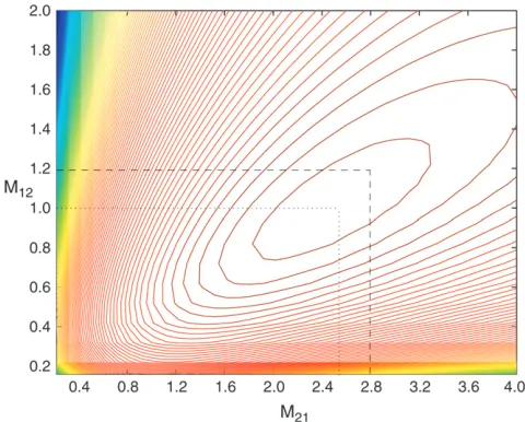
Migration models: Here we examine the perfor-mance of our approach at analyzing migration models. Note that we can estimate migration rates only relative to our choice of units for time, which is defined by our specification of the mutation rateu. Therefore, we fixuto its true value and look at estimates of the migration rates. Our approach for migration models is based on an ap-proximate likelihood, and first we need to check the validity of this approach. To do this we calculated the mean log-likelihood over a set of independent data. The shape of the mean log-likelihood governs the asymptotic behav-ior of the method, and in particular for an approximate likelihood method to produce consistent estimates it is re-quired that the mean log-likelihood curve attains its max-imum at the true value of the parameters (see Fearnhead 2003; Smithand Fearnhead2005, for further discussion). Thus an important property of an approximate-likelihood method is that the mean log-likelihood curve attains its maximum at a value close to the true value.
Figure 3.—Histograms of the samples of the
We simulated 100 coalescent trees with sample size ofm¼10 from the migration model withD¼2 demes,
N1¼3000,N2¼7000,M12¼1.2, andM21¼2.8. The
mutation rate used was u ¼30. For each data set we based inferences on 2000 sets of coalescence times sim-ulated from (3), again withfset to the value that maxi-mizes (5). We have estimated the mean log-likelihood at a grid of values ofM12,M21. A contour plot of this
log-likelihood surface is shown in Figure 4. The maximum of this curve is indeed close to the true parameter value (maximum atM12¼1.02,M21¼2.52). Similar results
are obtained for a range of migration models (results not shown).
In Table 1 we present results on the performance of our approach, obtained from simulated data of sizem¼ 10, 20 from the migration model withD¼2 demes for different values of the model parameters. We consider two sets of parameters: (a)N1¼N2¼5000,M12¼M21¼
0.4 and (b)N1¼3000,N2¼7000,M12¼1.2,M21¼2.8.
In each case we report the average of the most likely parameter values across 100 data sets, the standard er-rors of these estimates (in parentheses), and the associ-ated coverage of the 95% likelihood-based confidence intervals (C.I.’s). The average CPU cost of analyzing a data set on our laptop PC is 30 sec for them¼10 case and 50 sec for them¼20 case.
The method does have a bias, as can be seen in Figure 4 and Table 1; however, this bias is small compared to the standard error of the estimates and thus has a very small contribution to the mean square error of the estimator. The coverage properties of the confidence intervals vary notably between cases a and b; the reason for this is unclear. In this case it appears that the approximate-likelihood method performs much better and more robustly in terms of point estimates than in terms of assessing uncertainty in those estimates.
For comparison we reanalyzed them¼10,u¼15,M12¼ M21 ¼ 0.4 data sets using genetree (Griffiths and
Tavare´ 1994b; Bahloand Griffiths1998), which ap-proximates the true likelihood curve. To use a single run of genetree required that we fix the relative population sizes in the two populations. So we ran genetree and reran our approach assuming that bothuand the rela-tive population sizes were known and considered esti-mates of the single migration parameter. To implement genetree requires the choice of a driving value for the migration rate, and rather than choose a single value we ran genetree for five different values, ranging from 0.2 to 1.0, and averaged the likelihood curves across those obtained for each value. We ran genetree for 100,000 iterations for each driving value, which took around two Figure 4.—Contour plot of the mean log-likelihood
surface ofM12,M21obtained from 100 simulated coalescent
trees with sample sizem¼10 under the migration model with D¼2 demes (each contour corresponds to 0.05 units of log-likelihood). The mutation rate used wasu¼30. Shown are the true parameter values, M12 ¼ 1.2 and M21 ¼ 2.8, and
the values that maximize the surface, Mˆ12¼1:02 and
ˆ
M21¼2:52.
TABLE 1
Performance of our approximate-likelihood approach for simulated data under the migration model withD¼2 demes for scenarios (a)N1¼N2¼5000,M12¼M21¼0.4 and
(b)N1¼3000,N2¼7000,M12¼12,M21¼28
Case a Case b
m u Mˆ12 Coverage (%) Mˆ21 Coverage (%) Mˆ12 Coverage (%) Mˆ21 Coverage (%)
10 15 0.46 100 0.48 100 1.02 92 2.50 89
(0.26) (0.26) (0.64) (1.30)
10 30 0.42 100 0.46 100 1.08 95 2.62 97
(0.22) (0.26) (0.62) (1.22)
20 15 0.36 99 0.38 99 1.04 87 2.42 82
(0.24) (0.24) (0.72) (1.46)
20 30 0.38 97 0.38 97 1.06 90 2.66 88
(0.30) (0.30) (0.70) (1.36)
orders of magnitude longer to run than our approach. The median of ESSs of the estimate of the likelihood at the true migration rate was 15 across the 100 simulations (in comparison with an ESS of.1000 for our method). The estimates from the two methods were highly correlated (correlation coefficient 0.75). The root mean square error of our estimates was20% smaller than that of genetree. This suggests that for this case the Monte Carlo error within the genetree estimates of the likelihood curves is affecting the estimates of the migration rates more than the approximation error of our likelihood approach.
Continuous spatial models:Finally we present results for the continuous spatial models. Again here we can estimate the parameters of the spatial model only rel-ative to the mutation rateu. Therefore, we fix the
param-eters of the demographic model to their true values and look at estimates of the spatial parameters.
First, we check the validity of the approximate likeli-hood through calculating the mean log-likelilikeli-hood for a range of parameters. For each set of parameters we sim-ulated 100 data sets and then used our approximate ap-proach withK¼5000 to estimate the likelihood curve of
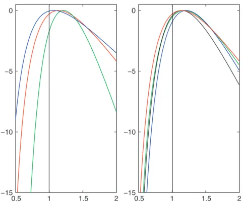
s, the parameter governing the rate of spatial dispersion, and to obtain samples from the posterior distribution of the location of the MRCA. Combining information from all of the 100 simulated trees we estimated the average log-likelihood at a grid of values ofs. Figure 5 shows the resulting mean log-likelihood curves for a range of val-ues of the sample size,m, the mutation rate,u, and the population growth parameter,b. In each cases¼1. The accuracy of the method appears to be primarily de-pendent onm, with the asymptotic bias of the method increasing asmincreases (as the value ofsfor which the maximum of the mean log-likelihood curve is attained gets further away froms¼1 asmincreases).
In Table 2 we present a summary of the estimates ofs
across the 100 data sets for each set of parameter values; and in Table 3 we give the root mean square error of the estimate of the position of the MRCA (these estimates had negligible bias); due to symmetry we show only the root mean square error for estimating one coordinate of the position.
We see that the estimates ofsare accurate for values ofmup to 10, and any bias is small relative to the stan-dard error of the estimator; beyond this we note a bias in our estimates, and the root mean square error actually increases when we move fromm¼10 tom¼40. Coverage properties also appear good for values ofmup to 10; but beyond this the confidence intervals are substantially anti-conservative. The values ofbanduappear to have little effect on the results. These results are consistent with those from Figure 5, with the bias of the estimator starting to dominate its performance for m¼20 and particularly form¼40.
Figure5.—Plots of the log-likelihood surface ofsfor a range
of parameter values, each obtained from 100 simulated data sets. Left-hand plot:u¼15,b¼1, andm¼10 (blue);m¼20 (red); andm¼40 (green). Right-hand plot:m¼20,u¼30, andb¼1 (black);u¼30,b¼2 (blue);u¼15,b¼1 (red); andu¼15,
b¼2 (green).
TABLE 2
Performance of our conditional-likelihood approach at estimatingsfor the spatial model
b¼1 b¼2
m u EðsˆÞ RMSE Coverage (%) EðsˆÞ RMSE Coverage (%)
5 2 0.99 0.45 95 1.00 0.42 96
5 5 1.09 0.46 93 0.99 0.38 94
10 5 1.02 0.28 95 1.04 0.29 95
10 15 1.05 0.24 94 1.03 0.23 94
20 15 1.13 0.22 83 1.18 0.26 79
20 30 1.14 0.27 79 1.20 0.29 73
40 15 1.22 0.31 57 1.23 0.30 51
40 30 1.22 0.30 45 1.28 0.32 40
We report the mean of the estimates ofs(truths¼1), the root mean square error of the estimates, and the coverage probability of 95% approximate confidence intervals. (The grid ofs-values ranged from 0 to 4 form¼
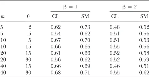
For comparison with our estimate of the position of the MRCA, we also calculated a simple unbiased esti-mate for each data set, which is obtained by taking the average of the locations of the sample. The root mean square error of one coordinate of the position is also shown in Table 3. Our approach is uniformly more accurate—with quite notable reduction in root mean square error for m ¼ 20 and m ¼ 40. Note that the estimates are more accurate forb¼2 than forb¼1 due to the tree being shorter and thus the spatial spread of the data being less.
One approach to reduce the bias of estimates for the
m¼20 andm¼40 cases is to use a composite likelihood. We tried a simple approach: For them¼20 case we split the data into two disjoint subsamples of size 10; and for them¼40 case we split the data into four disjoint sub-samples of size 10. For both cases we then calculated the log-likelihood for each subsample of size 10 and av-eraged this log-likelihood across the two, or the four, subsamples. We calculated our estimate ofsas the value that maximized this average log-likelihood curve. (Con-fidence intervals were calculated by treating the average log-likelihood curve as a standard log-likelihood curve.) The results are shown in Table 4. The bias and root mean square error of the estimates are substantially
re-duced for this approach, and also the coverage proba-bilities are much closer to 95%.We investigated using more, but nondisjoint, subsamples and found no im-provement in the estimates. We also tried using smaller subsamples (e.g., four disjoint subsamples of size 5 for the m¼20 case), but obtained worse performance in this case.
To demonstrate the advantage of postprocessing a sample of genealogical trees, rather than conditional analysis based on a single tree, we considered the alter-native approach of inferringsgiven a single estimate of the genealogy. Such an approach (i) obtains an estimate of the coalescent timesˆtusing the genetic data and (ii) bases inference on the conditional likelihoodpðxjˆt;sÞ. We used the maximum-likelihood estimator ofˆt(which for these models can be calculated using the method of Meligkotsidouand Fearnhead2005).
Here we present results for them¼2 andm¼5 cases, although similar results are obtained for larger values ofm. One difficulty with using the maximum-likelihood estimate oftis that the estimate of the coalescence time for two identical sequences is 0, which is inconsistent with chromosomes sampled from distinct locations. Thus in our analysis below we simulate data conditional on a sample having no identical sequences. We do not take account of this conditioning when analyzing the data.
Figure 6 gives probability–probability (PP) plots of the likelihood-ratio statistics for testing s ¼1 against draws from a chi-square distribution with 1 d.f. We show this plot as this PP plot is related to the coverage prop-erties of confidence intervals for the parameter, and if the likelihood-ratio statistic is approximately distributed as a chi-square distribution with 1 d.f., then it shows that the likelihood method is correctly quantifying the un-certainty in the parameter. This analysis is slightly com-plicated for them¼2 case, as the sample size is too small for the asymptotic limit of the likelihood-ratio statistic to be a very good approximation—thus we also show the PP plot for the likelihood-ratio statistic conditional on knowing the true coalescence time. For each value of
u we give PP plots for the new approximate-likelihood method, the conditional analysis for the data sets with at least one segregating site. For smaller values ofuthe
TABLE 4
Performance of our composite-likelihood approach at estimatingsfor the spatial model
b¼1 b¼2
m u EðsˆÞ RMSE Coverage (%) EðsˆÞ RMSE Coverage (%)
20 15 1.01 0.22 96 1.02 0.25 93
20 30 0.98 0.19 95 1.00 0.20 95
40 15 0.94 0.23 92 0.99 0.24 95
40 30 0.96 0.21 91 0.93 0.18 95
We report the mean of the estimates ofs(truths¼1), the root mean square error of the estimates, and the coverage probability of 95% approximate confidence intervals. (We split the data into disjoint subsamples of size 10. The grid ofs-values ranged from 0 to 2.)
TABLE 3
Performance of our conditional likelihood (CL) method and the sample mean (SM) at estimating the position of the MRCA
b¼1 b¼2
m u CL SM CL SM
5 2 0.62 0.73 0.48 0.52
5 5 0.54 0.62 0.51 0.56
10 5 0.67 0.70 0.51 0.53
10 15 0.66 0.66 0.55 0.56
20 15 0.61 0.66 0.52 0.58
20 30 0.56 0.62 0.52 0.59
40 15 0.66 0.69 0.46 0.51
40 30 0.68 0.71 0.55 0.62
approach that conditions on the maximum-likelihood estimate (MLE) for the coalescence time substantially underestimates the uncertainty of the estimate fors. As
uincreases the distribution of the likelihood-ratio (LR) statistic approaches the distribution of the LR statistic conditional on the true value of the coalescence time.
The effect of conditioning on the MLE of the times is less pronounced on the point estimates ofs. For the
m¼5 case, the two sets of MLEs are highly correlated (correlation ¼ 0.96) and give almost identical root mean square errors, although conditioning on the MLE appears to give slight underestimates ofs. A measure of the efficiency of our approach can be seen by looking at the correlation of the estimates from our method with those conditional on the true coalescence times; this again is high (correlation¼0.80). A related idea is used for inferring species trees in Edwardset al. (2007).
DISCUSSION
We have considered postprocessing of samples of ge-nealogies, in particular to learn about the demographic parameters for a sample and the robustness of inference to changes in the demographic model. While in our applications we have considered infinite-sites data from a nonrecombining region of DNA, but the ideas can be applied much more generally. (For example, for the variable population size analysis, changing the method of simulating the data will affect only step B of the algo-rithm, with the denominator of the importance-sampling weights being the prior of the model under which the sample of genealogies was generated.) All that is required is that there is computational machinery (e.g., MCMC algorithms) that can produce samples of genealogies for
the data. For example, analysis of more general muta-tion models is possible using the Bayesian phylogenetic packages such as MrBayes (Ronquistand Hulsenbeck 2000) and Bambe (Largetand Simon1999), while anal-ysis of (recombining) bacterial multilocus sequence typing data is possible using ClonalFrame (Didelot and Falush2007).
We first considered inference for a variable popula-tion size and robustness of inference of coalescence times to changes in the model for the population size. An importance-sampling approach, which is ‘‘exact’’ in the limit as the computational cost increases, is possible here. In practice the efficiency of this method will de-pend on the sample size and the mutation rate, with ef-ficiency decreasing as sample size increases or mutation rate decreases. Our results suggest that this approach is practicable for sample sizes of up to 50 chromosomes. The advantage of this postprocessing is that it enables a data set to be analyzed quickly under a range of different models. As such we view that this approach will be useful in terms of a preliminary analysis of a potentially large data set. We can first subsample an appropriate number of chromosomes (of the order of 10–50) and analyze these under a variety of models. This will help inform us as to what are the appropriate models for analyzing the complete data (using a more dedicated/computation-ally intensive approach) and also give insights as to how robust the results about the coalescence times of the tree will be.
We also considered inference in structured populations: both discrete subpopulations and continuous spatial mod-els. There are similarities in the approximate-likelihood approach we consider for both of these cases. We first simulate a sample of genealogies and then average over Figure 6.—Probability–
probability (PP) plots of a
x2
1-distribution against the
likelihood-ratio (LR) statistics for (red) our conditional like-lihood method, (blue) analysis conditional on the maximum-likelihood estimate of the co-alescence times, and (green) analysis conditional on the true coalescence times. a–c are based on 1000 data sets, with m¼ 2; b ¼ 1; and (a)
u¼1, (b)u¼2, and (c)u¼
the conditional likelihood of the spatial data given the genealogy. (For the migration model we also use an ap-proximate conditional likelihood, which is equivalent to allowing the population sizes in the demes to fluctuate through time.) This approach implicitly assumes a con-ditional independence structure to the data: that the spatial and genetic data are conditionally independent given the genealogy. As such our model assumes a prior for the genealogy and then conditional models for the spatial/genetic data given the genealogy. The prior for the genealogy is that assumed within our computational method for producing the sample of genealogies, in our case the phylogenetic prior described inmethods; al-though alternative methods for simulating the geneal-ogies could be used that assume different priors. For the continuous spatial model, if we had chosen our prior to be that used to simulate the data (coalescent under ex-ponential growth), then our approach gives a simulation-consistent approach for calculating the true likelihood of the data. The results we presented thus give an idea of the robustness of our approximate-likelihood method to the choice of the wrong prior. For practical applica-tions, where the true choice of the prior (or equivalently model) for the genealogy is not known, the robustness of any method to the choice of this prior will be of par-amount importance. In most scenarios that we exam-ined the bias of the approximate-likelihood method is small compared to the standard error of the estimate. In general asmincreases, biases increase. This is because as
mincreases the genealogical prior we use does not cor-rectly capture the distribution of some of the coales-cence times, and this then starts to introduce notable biases into the method.
For implementation of our approximate-likelihood method to new data and models it is important to know for what sample sizes the method will produce good statistical properties, such as small biases and appropri-ate coverage probabilities for confidence intervals. Cur-rently, to evaluate this accurately will require some form of simulation study chosen to be appropriate for the models and data being considered. The results we have presented give insight into for what sample sizes the method will perform well. Our method can be applied to large data sets using a composite-likelihood approach. A large data set can be split into smaller subsamples (with the possibility of each chromosome appearing in many subsamples), with the approximate log-likelihood calculated for each subsample, and these approximate log-likelihood curves can be combined through averag-ing them together. An estimate of the parameter(s) is given by the value(s) that maximize this composite log-likelihood. The performance of such a method is governed by the shape of the mean of the log of the approximate likelihood, as shown in Figure 5 (see Fearnhead2003). We tested out one implementation of this composite-likelihood approach for the continuous spatial model and found it to perform well using subsamples of size 10.
In particular, a pairwise-likelihood approach is likely to be a simple and flexible method for analyzing con-tinuous spatial data sets (currently there are few methods for analyzing such models). For such a pairwise ap-proach it is simple to allow for quite general models of the spatial spread of the population through time; all that is required is the specification of a family of den-sities,p(x1,x2;t), for the probability of two chromosomes
that share a common ancestor at timetin the past being located at positionsx1andx2.
This work was supported by Engineering and Physical Sciences Research Council grant R91724 and by an Engineering and Physical Sciences Research Council Springboard Fellowship to P.F.
LITERATURE CITED
Bahlo, M., and R. C. Griffiths, 1998 Inference from gene trees in
a subdivided population. Theor. Popul. Biol.57:79–95.
Beerli, P., and J. Felsenstein, 1999 Maximum-likelihood estimation
of migration rates and effective population numbers in two
pop-ulations using a coalescent approach. Genetics152:763–773.
Brooks, S. P., I. Manopoulouand B. C. Emerson, 2007 Assessing
the affect of genetic mutation: a Bayesian framework for deter-mining population history from DNA sequence data, pp. 25– 50 inBayesian Statistics 8, edited by J. M. Bernardo, M. J. Bayarri,
J. O. Berger, A. P. Dawid, D. Heckerman, A. F. M. Smithand
M. West. Oxford University Press, Oxford.
Coop, G., and R. C. Griffiths, 2004 Ancestral inference on gene
trees under selection. Theor. Popul. Biol.66:219–232.
Didelot, X., and D. Falush, 2007 Inference of bacterial
microevo-lution using multilocus sequence data. Genetics175:1251–1266.
Drummond, A. J., A. Rambaut, B. Shapiro and O. G. Pybus,
2005 Bayesian coalescent inference of past population
dynam-ics from molecular sequences. Mol. Biol. Evol.22:1185–1192.
Edwards, S. V., L. Liuand D. K. Pearl, 2007 High-resolution
spe-cies trees without concatenation. Proc. Natl. Acad. Sci. USA104:
5936–5941.
Emerson, B. C., and G. M. Hewitt, 2005 Phylogeography. Curr. Biol.
15:367–371.
Fearnhead, P., 2003 Consistency of estimators of the
population-scaled recombination rate. Theor. Popul. Biol.64:67–79.
Fearnhead, P., and P. Donnelly, 2001 Estimating recombination
rates from population genetic data. Genetics159:1299–1318.
Fearnhead, P., and P. Donnelly, 2002 Approximate likelihood
methods for estimating local recombination rates (with discus-sion). J. R. Stat. Soc. Ser. B64:657–680.
Fearnhead, P., and L. Meligkotsidou, 2004 Exact filtering for
partially-observed continuous-time Markov models. J. R. Stat.
Soc. Ser. B66:771–789.
Felsenstein, J., 1975 A pain in the torus: some difficulties with the
model of isolation by distance. Am. Nat.109:359–368.
Felsenstein, J., 1981 Evolutionary trees from DNA sequences: a
maximum likelihood approach. J. Mol. Evol.17:368–376.
French, N. P., M. Barrigas, P. Brown, P. Ribiero, N. J. Williams
et al., 2005 Spatial epidemiology and natural population struc-ture of campylobacter jejuni colonising a farmland ecosystem.
Environ. Microbiol.7:1116–1126.
Griffiths, R. C., and P. Marjoram, 1996 Ancestral inference from
samples of DNA sequences with recombination. J. Comput. Biol.
3:479–502.
Griffiths, R. C., and S. Tavare´, 1994a Sampling theory for neutral
alleles in a varying environment. Philos. Trans. R. Soc. Lond. Ser.
B344:403–410.
Griffiths, R. C., and S. Tavare´, 1994b Simulating probability
dis-tributions in the coalescent. Theor. Popul. Biol.46:131–159. Kuhner, M. K., J. Yamatoand J. Felsenstein, 1998 Maximum
likeli-hood estimation of population growth rates based on the
coales-cent. Genetics149:429–434.
Kuhner, M. K., J. Yamatoand J. Felsenstein, 2000 Maximum
likeli-hood estimation of recombination rates from population data.
Larget, B., and D. L. Simon, 1999 Markov chain Monte Carlo
algo-rithms for the Bayesian analysis of phylogenetic trees. Mol. Biol.
Evol.16:750–759.
Liu, J. S., 1996 Metropolised independent sampling with
compari-sons to rejection sampling and importance sampling. Stat.
Com-put.6:113–119.
Meligkotsidou, L., and P. Fearnhead, 2005 Maximum likelihood
estimation of coalescence times in genealogical trees. Genetics
171:2073–2084.
Rannala, B., and Z. Yang, 1996 Probability distribution of
molecu-lar evolutionary trees: a new method of phylogenetic inference. J. Mol. Evol.43:304–311.
Ronquist, F., and J. P. Hulsenbeck, 2000 MrBayes3: Bayesian
phy-logenetic reconstruction under mixed models. Bioinformatics
19:1572–1574.
Rue, H., and L. Held, 2005 Gaussian Markov Random Fields: Theory
and Applications. CRC Press/Chapman & Hall, Cleveland; Boca Raton, FL/London; New York.
Shen, P., F. Wang, P. A. Underhill, C. Franco, W. Yanget al.,
2000 Population genetic implications from sequence variation
in four Y chromosome genes. Proc. Natl. Acad. Sci. USA 97:
7354–7359.
Smith, N. G. C., and P. Fearnhead, 2005 A comparison of three
es-timators of the population-scaled recombination rate: accuracy
and robustness. Genetics171:2051–2062.
Srinivasan, R., 2002 Importance Sampling. Springer, New York.
Stephens, M., and P. Donnelly, 2000 Inference in molecular
pop-ulation genetics (with discussion). J. R. Stat. Soc. Ser. B62:605– 655.
Templeton, A. R., E. Boerwinkleand C. F. Sing, 1987 A cladistic
analysis of phenotypic associations with haplotypes inferred from restriction endonuclease mapping. I. Basic theory and an analysis
of alcohol dehydrogenase activity in Drosophila. Genetics117:
343–351.
Underhill, P. A., G. Passarino, A. A. Lin, P. Shen, M. Lahret al.,
2001 The phylogeography of Y chromosome binary haplotypes
and the origins of modern human populations. Ann. Hum.
Genet.65:43–62.
Wilkins, J. F., 2004 A separation-of-timescales approach to the
coalescent in a continuous population. Genetics 168: 2227–
2244.
Wilkins, J. F., and J. Wakeley, 2002 The coalescent in a continuous,
finite, linear population. Genetics161:873–888.
Wright, S., 1943 Isolation by distance. Genetics28:114–138.
Communicating editor: R. Nielsen
APPENDIX
The prior (2) can be obtained by simulatingsfrom the prior with f¼1 and then letting t¼fs. Thus if we defineSandsij’s to satisfyT¼fSandtij¼fsij, so they are the respective times obtained froms, we get that
CovðXi;XjÞ ¼s2fðSsijÞ:
Thus the intuition behind the result is that, as under the prior, the data are solely informative about the product
s2f, and using the scale invariance prior forfwill result
in no information abouts. Formally we use the fact that
pðxjsÞ ¼
ð ð
pðxjs;f;sÞpðfÞdfpðsÞds:
We consider the integral with respect tof, assuming a givens, and demonstrate that this does not depend on
s, from which the fact thatp(xjs) does not depend on
sfollows. For notational simplicity we assumem¼0 in the following.
Now, for our given s, let S be the covariance ma-trix obtained whens¼f¼1, soSij¼(Ssij) fori,j¼ 1,. . .,m. Further letQ¼S1
andA¼xT
Qx/2. Then
ð
pðxjs;f;sÞpðfÞdf
}
ð
ðs2fÞm=2expfA=ðs2fÞgf1df
¼sm
ð
gm=21expfgA=ðs2Þgdg
¼smGðm=2ÞðA=s2Þm=2: