The Structure of Linkage Disequilibrium Around a Selective Sweep

DOI: 10.1534/genetics.106.062828

The Structure of Linkage Disequilibrium Around a Selective Sweep

Gil McVean

1

Department of Statistics, University of Oxford, Oxford OX1 3TG, United Kingdom

Manuscript received June 30, 2006 Accepted for publication December 24, 2006

ABSTRACT

The fixation of advantageous mutations by natural selection has a profound impact on patterns of linked neutral variation. While it has long been appreciated that such selective sweeps influence the frequency spectrum of nearby polymorphism, it has only recently become clear that they also have dramatic effects on local linkage disequilibrium. By extending previous results on the relationship between genealogical structure and linkage disequilibrium, I obtain simple expressions for the influence of a selective sweep on patterns of allelic association. I show that sweeps can increase, decrease, or even eliminate linkage dis-equilibrium (LD) entirely depending on the relative position of the selected and neutral loci. I also show the importance of the age of the neutral mutations in predicting their degree of association and describe the consequences of such results for the interpretation of empirical data. In particular, I demonstrate that while selective sweeps can eliminate LD, they generate patterns of genetic variation very different from those expected from recombination hotspots.

S

ELECTIVE sweeps, in which a beneficial mutation is swept to fixation in a population by natural selec-tion, have a profound impact on patterns of linked genetic variation through what is known as the hitch-hiking effect (Maynard Smith and Haigh 1974).

Although simple in concept, studies of the process con-tinue to uncover novel and unusual properties that have direct implications for the detection of such events from empirical data. For example, the realiza-tion that the interacrealiza-tion of hitchhiking with recombi-nation can lead to an excess of high-frequency-derived mutations (Fayand Wu2000) gave novel insights into

the well-known fact that hitchhiking can lead to a bias toward low-frequency polymorphism (Fuand Li1993;

Bravermanet al.1995). Recently, studies of the effects

of selective sweeps on patterns of linkage disequilib-rium (LD) have also identified characteristic, and per-haps surprising, patterns (Kim and Stephan 2002;

Przeworski 2002; Kim and Nielsen 2004; Reed and

Tishkoff 2005; Stephan et al. 2006). For example,

while sweeps can lead to an increase in LD while they are still in progress (Hudsonet al.1994; Sabetiet al.2002),

when the beneficial mutation has reached fixation, LD across the selected site is eliminated (Kimand Nielsen

2004; Stephanet al. 2006). Interpreting empirical

pat-terns of genetic variation in the light of such observations is therefore potentially confusing and raises important questions. For example, are positions at which LD is observed to break down rapidly the result of selective sweeps or recombination hotspots? Indeed, it has been

demonstrated that for certain population genetic meth-ods selective sweeps may be falsely interpreted as hots-pots of recombination (Reedand Tishkoff2005).

The aim of this article is to provide an intuitive inter-pretation of the effects of selective sweeps on patterns of LD, through considering the relationship between LD and the structure of the underlying genealogical history. Previous work has shown that there is a direct quantitative relationship between the magnitude of LD observed between a pair of neutral mutations and the correlation structure of the underlying genealogy (McVean2002). By using the conventional

approxima-tion that strong selective sweeps lead to short, star-like genealogies at the selected site, this theory is extended to examine the correlation structure between the ge-nealogies of neutral loci either separated by or adjacent to the selected site. Comparison with the results of stochastic simulation demonstrates that this theory pre-dicts the qualitative and, to some extent, quantitative, behavior of LD around a selective sweep. In addition, the theory identifies the importance of the age of neu-tral mutations (relative to the selected one) in deter-mining patterns of LD and predicts large differences in the nature of the breakdown of LD around a selective sweep and a recombination hotspot.

TWO-LOCUS IDENTITIES AND A GENEALOGICAL INTERPRETATION OF LD

Informally, LD between neutral alleles at two loci arises because of correlations in the genealogical his-tory of the two loci. Put another way, if the time to the MRCA (most recent common ancestor) for a pair of chromosomes at a given position,x, on the genome is

1_{Address for correspondence:Department of Statistics, 1 S. Parks Rd.,} Oxford OX1 3TG, United Kingdom. E-mail: [email protected]

informative about the time to the MRCA for the same pair of chromosomes at another genomic position, y (relative to any other pair of chromosomes), the alleles at the two loci are expected to show significant LD. However, different statistical measures of LD focus on different aspects of such correlation. Here we focus on one widely used two-locus measure of LD for biallelic loci, the square of the correlation coefficient in allelic state orr2 _{(Hilland Robertson1968). For a pair of}

biallelic loci, with alleles 0 and 1 at locusxand also 0 and 1 at locusy, the statistic is defined as

r2¼ D

2 11

f0df1dfd0fd1

D11¼f11 f1dfd1: ð1Þ

Here,f11is the sample frequency of the 11 haplotype and

f1dis the marginal sample frequency of the ‘‘1’’ allele at locusx. Note that for biallelic loci the value ofr2_{does not}

depend on which allele is assigned the value 1. Conse-quently, in what follows the subscript forDis omitted.

Ideally, we wish to calculate the expected value ofr2

between alleles at the two loci, conditioning on observ-ing at least one of each allele at each of the two loci in a sample of sizensequences:

E½r2 ¼E D

2

f0df

1dfd

0fd

1

jf0df

1dfd

0fd

1.0

: ð2Þ

There is, unfortunately, no simple expression for this expectation, although recent advances have been made in its numerical evaluation (Song and Song 2007).

However, it is possible to derive expressions for a related quantity, calleds2

d:

s2_d¼ E½D

2_jf

0df1dfd0fd1.0

E½f0df1dfd0fd1jf0df1dfd0fd1.0

ð3Þ

(Ohta and Kimura 1971). After this point the

con-ditioning on segregation at the two loci will be implicit. It can be shown through Monte Carlo simulation (Hudson 1985; McVean 2002) that Equation 3 is a

good approximation to the expectation ofr2_(i.e.,

Equa-tion 2) for large sample sizes and when rare variants are excluded.

Previous work (Strobeckand Morgan1978; Hudson

1985) showed that the statistic D2 _{can be rewritten in}

terms of two-locus identity coefficients:

D2¼Fij;ij2Fij;ik1Fij;kl: ð4Þ

To understand the two-locus identity coefficients, con-sider sampling four chromosomes at random with re-placement from a population and labeling themi,j,k, andl. The three terms on the right-hand side of Equa-tion 4 are, respectively, the probability that sequences iand j are identical in state at both sites xand y, the probability that sequencesiandjare identical at locusx

and that sequences i andkare identical at site y, and the probability that sequences iand j are identical at sitexand sequenceskandlare identical at sitey. These three configurations, which are referred to as A, B, and C, respectively, are central to the following discussion and are represented in Figure 1A. A similar expression applies to the sample statistic where the chromosomes are drawn (with replacement) from the sample (Hudson

1985). In small samples it is therefore possible thati,j, etc., are not distinct.

The key point about Equation 4 is that the expecta-tion ofD2_{can be written in terms of the expectation of}

these two-locus identity coefficients. Under the infinite-sites model, in which each polymorphism observed is the result of a single mutation event within the sample’s history, it is possible to relate the two-locus identities to the expectations of genealogical properties at the two loci (McVean2002). For example,

E½Fij;ij ¼

E½ðTxtijxÞðTytijyÞ

E½TxTy

; ð5Þ

Figure1.—(A) Two-locus configurations relating to

where Tx is the total time in the genealogy (i.e., the

sum of the branch lengths) at locus x and tx ij is the

coalescence time for sequences i and j at locus x. By obtaining similar expressions for the other two-locus identities and also the denominator of Equation 3, it was shown that

s2_d¼rðt

x ij;t

y

ijÞ 2rðtijx;t y

ikÞ1rðtijx;t y klÞ

ðCVxCVyÞ11rðtijx;t y klÞ

ð6Þ

(McVean2002), whererðtx ij;t

y

klÞis the Pearson

correla-tion coefficient between the coalescence time for se-quencesiandjat locusxand the coalescence time for sequenceskandlat locusyand CVxis the coefficient of

variation in the time to the most recent common an-cestor (MRCA) for a pair of randomly sampled chromo-somes at locusx, CVx¼

ffiffiffiffiffiffiffiffiffiffiffiffiffiffiffiffiffiffiffi Varðtx

ijÞ

q

=E½tx

ij. Note that there

are three correlations in Equation 6, relating to the three sample configurations (see Equation 4 and Figure 1A). The most important implication of Equation 6 is that it provides a quantitative approach for relating patterns of LD to features of the underlying genealogical his-tory. For example, demographic histories in which the population has increased, decreased, or remained con-stant in size influence LD both through their effects on the correlation structure of genealogies and through their effects on the coefficient of variation in time to the MRCA. For example, population growth reduces the coefficient of variation thus reducing LD, while pop-ulation bottlenecks increase the coefficient of variation, increasing LD. The theory can also be extended to con-sider more complex situations, for example, the case of a series of island populations connected by migration (Wakeleyand Lessard2003). In the next section, the

theory is extended to the case of a pair of neutral loci linked to a site that has undergone a complete selective sweep in which the beneficial mutation has just reached fixation in the population.

MODELING GENEALOGIES UNDER A SELECTIVE SWEEP

Looking back in time, a neutral locus on a single line-age at some genetic distanceR ¼4Ner from a selected

site (whereris the genetic map distance in Morgans and Neis the effective population size, assumed to be

dip-loid) can either recombine away from the selected mutation before its removal from the population, with probabilityp, or not, with probabilityq¼ 1p. The probability of ‘‘escape’’ is a function of the recombina-tion rate and the frequency trajectory of the selected mutation, itself a random variable determined by the scaled selection coefficientS¼4Nes. By approximating

the trajectory of the selected mutation by that of the deterministic expectation, it has been previously shown that

p1exp R

Sln 2Ne

ð7Þ

(MaynardSmithand Haigh1974; Kaplanet al.1989;

Stephan et al. 1992; Durrett and Schweinsberg

2004). Implicit within this formula is an expression for the age of the selected mutation:

tM

4 ln 2Ne

S : ð8Þ

As for all expressions relating to age, this is expressed in units of 2Negenerations. When there is more than a

single lineage to consider (i.e., a sample of sizen.1), the shape of genealogy under the selected mutation has to be considered. However, if a selective sweep is sufficiently strong, this genealogy can be approximated as a star phylogeny (MaynardSmithand Haigh1974;

Kimand Stephan2002) with the age of the common

ancestor, tM, taken from Equation 8 (Figure 1B).

Al-though this approximation can be criticized (Barton

1998; Durrett and Schweinsberg 2004; Etheridge

et al. 2006), it nevertheless has proved very useful in analytical treatments of hitchhiking, because of the resulting independence between lineages in whether they recombine away from the selected mutation.

A further simplifying assumption, tM>E½TMRCA, is

also made, whereTMRCAis the time until the MRCA for a

sample ofnchromosomes. Under the standard neutral model, E½TMRCA ¼2ð11=nÞ. Looking back in time,

the history of the sample can therefore be divided into two phases (Figure 1B). During the first ‘‘selection phase’’ the only events that can occur are recombination events that move neutral loci from the background of the selected allele to that of the ancestral, wild-type allele. The end of the selection phase is marked by the origin of the selected mutation at which point all chromosomes carrying the selected allele coalesce immediately, and the selected allele is removed. Sub-sequently, in the ‘‘neutral phase,’’ the history of the remaining lineages follows that of the standard neutral model. In the extreme, the selection phase can be considered instantaneous with respect to the timescale of the neutral coalescent process (i.e., tM0) and

therefore any mutations segregating must have oc-curred on the portion of the genealogy that predates the origin of selected mutation. Under this assumption if no lineages have recombined to the ancestral back-ground at a given distance from the selected site, there will be no polymorphism in the sample.

A, B, and C, is distributed at the start of the neutral phase. For example, consider configuration A where the selected site separates the two neutral loci (Figure 2). Depending on the distribution of recombination events that move a neutral locus from the selected to the ancestral background, this initial configuration can be transformed into any of 10 possible states at the end of the selected phase. The removal of the selected muta-tion subsequently transforms these 10 configuramuta-tions, through coalescence of those still carrying the selected mutation, to any of configurations A, B, and C or to ones where one or both of the neutral loci coalesce

(in-dicated by O in Figure 2). Details of the probabilities of each transition are given inappendixes aandb.

Once the transition probabilities to each possible state at the start of the neutral phase have been cal-culated, it is a simple matter to obtain expressions for the necessary genealogical statistics. In particular, for each starting configuration we can write the expectation of the product of the coalescence time at the two neutral loci as a function of these transition probabilities. For example,

ES½tijxt y

ij ¼fAAEW½tijxt y

ij1fABEW½tijxt y

ik1fACEW½tijxt y kl;

ð9Þ

wheref_ABis the probability that configuration A in the sampled chromosomes (all of which carry the selected mutation) results in configuration B at the start of the neutral phase. The subscript S on the left-hand side indi-cates that the expectation refers to the selected allele, while the subscript W on the right-hand side indicates that these expectations refer to the wild-type allele (i.e., the standard neutral expectations). Under the standard neutral model these quantities are known for different configurations of chromosomes. In particular,

EW½tijxt y ij ¼

36114R1R2 18113R1R2

EW½tijxt y ik ¼

24113R1R2 18113R1R2

EW½tijxt y kl ¼

22113R1R2

18113R1R2 ð10Þ

(Pluzhnikov and Donnelly 1996; McVean 2002).

Expressions similar to Equation 9 can be obtained for the other initial configurations B and C. Note that it is not necessary to include in Equation 9 a term for transi-tions to state O, as the expected product of coalescence times for this state is zero under the assumptiontM0.

Finally, because the configurations can be thought of as relating to subsamples (with replacement) from a sample of n sequences, there is a possibility that sequences i, j, k, and lmay not be distinct (the same sequence could be picked twice). A simple correction has to be made to the expectations,

E_S*½t_ijxt_ijy ¼ n1 n

ES½tijxt y ij

E_S*½t_ijxtiky ¼

n1 n

n2 n

ES½tijxt y ik1

1 n

n1 n

ES½tijxt y ij

E_S*½t_ijxt_kly ¼ n1 n

n2 n

n3 n

ES½tijxt y kl

14

n n1

n

n2 n

ES½tijxt y ik

1 2

n2 n1

n

ES½tijxt y

ij; ð11Þ

Figure2.—Transition probabilities for the two-stage model

of a selective sweep. The initial configuration (type A), where the selected mutation (solid circle) separates the two neutral loci (triangles), can be transformed into one of 10 different configurations at the end of the selection phase (the open cir-cle indicates the ancestral, unselected mutation). Probabilities for each transition are shown in terms ofpiandqi, respectively, the probability of a recombination event occurring in intervali

where n is the sample size (Hudson 1985; McVean

2002).

NEUTRAL LOCI SEPARATED BY THE SELECTED SITE

First, consider the case of two loci separated by the selected site and distant from it by recombination dis-tances of Rx andRy, respectively, such that the

proba-bilities of a lineage escaping the selective sweep arepx

and py, respectively. By considering the probability of

recombination in each interval it can be shown that

f_AA¼f_BA¼f_CA¼0

f_AB¼f_BB¼f_CB¼4pxqxpyqy

f_AC¼f_BC¼f_CC¼pxpyð2px12py3pxpyÞ ð12Þ

(seeappendix a). Consequently

ES½tijxt y

ij ¼ES½tijxt y

ik ¼ES½tijxt y

kl: ð13Þ

It follows that whatever the values ofRxandRy

s2 d¼

ES½tijxt y

ij 2ES½tijxt y

ik1ES½tijxt y kl

ES½tijxt y kl

¼0: ð14Þ

In other words, LD across the selected site (as measured bys2

d) is zero or at least no greater than background

levels caused by finite sample size. This result agrees with previous findings (Kimand Nielsen2004; Stephanet al.

2006) obtained by simulation and analysis of determin-istic models of selection. It is worth noting that a deter-ministic model (in which drift during the selection phase is ignored) is equivalent to assuming that no coalescent events occur during this period, the same assumption as is made here.

However, it is also worth noting that while LD may be zero, there is actually nonzero correlation in coales-cence time. For example, if Rx¼Ry¼R=2 and px¼

py¼p>1, it can be shown that

rðt_ijx;tijyÞ ¼rðtijx;t y

ikÞ ¼rðtijx;t y klÞ

6p

10113R1R2: ð15Þ

It is perhaps surprising that there should be nonzero correlation in the time to the MRCA at the two neutral loci, but yet no LD. The nonzero correlation arises because lineages that escape the sweep will have low, though nonzero, correlations in the time to the MRCA resulting from the neutral part of their ancestry. For example, Equation 15 is derived by noting that when the recombination rate is low, the most probable configu-ration that arises in which both neutral loci escape the sweep is configuration B (this is true for all initial configurations). However, each initial configuration requires exactly the same set of recombination events to occur to reach configurations B and C at the start of the neutral phase, so the resulting correlation structure

is the same for each initial configuration, and there is no LD.

NEUTRAL LOCI ON THE SAME SIDE OF THE SELECTED LOCUS

Now consider a pair of loci that are both on the same side of the selected site, with the nearer (or proximal),x, being at recombination distanceRx and the more

dis-tant (or distal),y, being at a recombination distanceRy

from x. In this situation the different initial configu-rations have different probabilities of resulting in each configuration at the start of the neutral phase. For ex-ample, configuration A can escape the sweep through a single recombination, while configuration C requires a minimum of two recombination events to escape the sweep. By considering the effect of recombination events occurring in each part of each chromosome during the selection phase (seeappendix b) it follows that for

con-figuration A

f_AA¼pxð2pxÞqy2

f_AB¼2pxð2pxÞpyqy

f_AC¼pxð2pxÞp2y: ð16Þ

For configuration B

f_BA¼pxqx2qy2

f_BB¼pxqy½4qx2py1pxð32pxÞ

f_BC¼pxpy½pxð34pyÞ 2px2qy12py: ð17Þ

While for configuration C

f_CA¼0

f_CB¼4pxqx2qyð1qxqyÞ

f_CC¼pxð1qxqyÞ½ð23pxÞð1qxqxÞ12px: ð18Þ

The mean and variance of the time to coalescence at each locus are

E½tx ¼1qx2

VarðtxÞ ¼2E½tx E½tx2

E½ty ¼1 ðqxqyÞ2

VarðtyÞ ¼2E½ty E½ty2: ð19Þ

These results can be used to derive numerical expres-sions for Equation 6 for various parameter values (Fig-ure 3). However, several important feat(Fig-ures of the results can be identified. First, whenpx>1 it follows that

rðt_ijx;t_ijxÞ 2rðt_ijx;t_ikxÞ 1

2 px

px1py 1=2

336114Ry1R

2 y

18113Ry1Ry2

Under this approximation, Equation 6 evaluates at zero. However, whenpx>1, such thatnpx,1, it is also critical

to account for the finite sample size, such thati,j,k, andl are not necessarily distinct. Under these conditions a good approximation for the expected LD is

s2_d 1

11npyðð24113Ry1Ry2Þ=ð36114Ry1Ry2ÞÞ :

ð21Þ

Equation 21 predicts that conditional on observing polymorphism at the linked neutral loci there will be perfect correlation (i.e., r2 _{¼1) between the alleles if}

there is no recombination between them (Figure 3). This result can be understood by noting that the most probable way in which polymorphism will be observed if px>1 is if a single lineage escapes the selective sweep.

Any neutral mutations must occur during the neutral phase, in which only two lineages will be present (the lineage leading to the MRCA of the selected mutation and the escaped lineage), leading to perfect association (in effect the mutations will occur on the same branch of the unrooted genealogy, as in Figure 1B). Another prediction of Equation 21 is that the magnitude of LD decreases rapidly as the recombination rate between the neutral loci increases. Indeed for moderate to large sample sizes it should decrease below that expected for an identical pair of neutral sites unaffected by a sweep (Figure 3). From a genealogical perspective, any re-combination events occurring between the two neutral loci will rapidly lead to a breakdown in the correlation of the genealogies at the two positions. Informally, the effect can also be understood in terms of allele fre-quency. Whenpx>1, polymorphism at the proximal

lo-cus is most likely to be in the form of a singleton (i.e.,

one chromosome differs from all the others). Recom-bination between the proximal and the distal loci will allow nonsingleton polymorphism at the distal locus and this is likely to show weak LD with the singleton allele at the proximal locus.

As the recombination rate between the proximal neutral locus and the selected site increases, the impact of the selective sweep diminishes and the LD between the neutral loci approaches that expected under the neutral model. However, the two key features of the pattern remain. First, if the neutral loci are very closely linked, LD is generally increased relative to the neutral expectation. Second, weakly linked neutral loci show a small decrease in LD relative to the neutral case (Figure 3). Both features can be explained by the above reasoning.

INCORPORATING NEUTRAL MUTATIONS YOUNGER THAN THE SELECTED MUTATION

So far, it has been assumed that the time to the origin of the beneficial mutation is approximately zero, such that any polymorphism found in the sample has to be older than the selected mutation. However, when the probability of a lineage escaping the selective sweep by recombination is low the expected time in genealo-gies in which no recombination occurs is considerable relative to the total expected time in the genealogy. Con-sequently, when px>1 it is relatively likely that

poly-morphism observed in a sample that has experienced a selective sweep may be more recent than the selected mutation. From the genealogical perspective, consider-ing such recent mutations is equivalent to settconsider-ingtM.0.

Because no coalescent events occur during the selected phase, the only influence of a nonzero value oftM is to

increase the expected coalescence time (it has no effect on the correlations in coalescence time or variance) and consequently decrease the coefficient of variation in coalescence time, thus reducing LD. When the neutral loci are either side of the selected site LD is low anyway, so inclusion of recent mutation has little or no impact on LD. However, when the two neutral loci are on the same side of the selected mutation recent mutation can have a considerable impact on LD, because neutral mutations older than the selected one will typically show strong LD if they are themselves tightly linked (as described above). To get an idea for the importance of including recent mutations, note that when npx,1,

typically at most one lineage will escape the sweep and the contribution of the neutral phase to the expected time in the genealogy of the sample is 2npx. Under

these same conditions the total length of the genealogy within the selected phase is ntM4npx= Rx.

Conse-quently, the probability that an observed neu-tral mutation at the proximal locus is older than the selected mutation is Rx=ð21RxÞ. In humans the

Figure 3.—The effect of a nearby selective sweep on LD

between a pair of linked neutral loci. Numerical evaluation of Equation 6 is shown with the correction for finite sample size in the case where both neutral loci are on the same side of the selected site.s2

dis shown as a function of the

recombi-nation rate,R¼ 4Ner, between the neutral loci (x-axis) and

average recombination rate isR ¼0:4=kb in European populations (Myerset al.2005), so that a polymorphism

5 kb from the selected site will have only a 50% prob-ability of being older than the selected mutation.

Figure 4 shows that inclusion of recent mutations has a marked effect ons2

d. When the recombination rate

between the neutral loci is zero, mutations older than the selected one are predicted to show (and do show) monotonically decreasing LD as a function of increas-ingpx. However, when recent mutations are considered,

LD very close to the selected site is near zero whenpxis

small. LD increases aspxincreases, exceeding the

neu-tral expectation at intermediate values ofpx. Finally, as

px approaches one, the expected LD decreases toward

neutral expectation. The nonmonotonic relationship between the distance of the neutral loci from the se-lected site and the strength of LD is actually more marked in the simulations (see below) than in the theor-etical predictions. Qualitatively similar patterns are predicted when the neutral loci are only partially linked (data not shown).

STOCHASTIC SIMULATION

To examine the accuracy of the results obtained here, Monte Carlo simulations were performed under two different models for the selective sweep. In series A, the effects of a selective sweep were simulated under the approximate model used as the basis of the analytical results. Specifically the genealogical history is divided into two phases: a phase of durationtMduring which the

only events that can occur are recombination events that move lineages from the selected to the wild-type background, a point of instant coalescence between all lineages still carrying the selected allele, and a neutral phase. In series B, fully stochastic models of selective sweeps were simulated using the program SelSim (Spencer and Coop 2004). Briefly, the method first

simulates a stochastic trajectory for the selected muta-tion backward in time using a diffusion approximamuta-tion (Coop and Griffiths 2004) and then subsequently

performs a structured coalescent simulation

condi-tional on the trajectory. By performing the two series of simulations it is possible to examine both the ac-curacy of Equation 6 as an approximation to the ex-pectation of r2 _{and the accuracy of the approximate}

model for selective sweeps. For efficiency simulations were carried out by placing mutations uniformly on the simulated genealogies at loci x and y and the ith simulation was assigned a weight given by the product of the total branch lengths at each site, wi¼TxiT

i y.

Expected values ofr2 _{are estimated from the weighted}

average over $105 _{simulations for each parameter}

combination.

Where the selected site separates the two neutral loci the extent of association between the neutral loci in the series A simulations was, as predicted, no higher than background (data not shown). When the selected site does not separate the neutral loci the results are highly sensitive to assumptions about the duration of the selec-tive phase (Figure 4, A and B; note that there is no recombination between the neutral loci). In Figure 4A it was assumed that the age of the selected mutation was negligible compared to the age of the neutral geneal-ogy, tM¼0. In Figure 4B, the age of the selected

mu-tation was fixed attM¼0:1053, the average obtained by

fully stochastic simulation withS¼400 and a sample size of 20. There are two key features of these results. First, in both cases Equation 6 typically overestimates the ex-pected value ofr2_{, although the expression is accurate}

when the probability of escape is low. The second key point is the difference the inclusion of recent neutral mutations makes. As predicted, mutations older than the selected one do typically show very strong LD. How-ever, when the probability of escaping the selective sweep is very low, recent neutral mutations make the majority contribution to LD, such that the average value ofr2 _{is very low.}

Figure 5 shows the comparison between the analytical results and the average value ofr2 _{calculated from the}

fully stochastic simulations. These give qualitatively the same results as those obtained under the approximate model of a selective sweep. When the selected mutation separates the neutral mutations there is no LD between

Figure 4.—The effects of a nearby selective

sweep on a pair of completely linked neutral mu-tations (A) when only neutral mumu-tations within the neutral phase are considered and (B) when neutral mutations can also occur during the se-lected phase. In each plot the solid line and shaded circles indicate numerical evaluation of Equation 6 and the dotted line and solid circles indicate the results of stochastic simulation car-ried out under the assumed model (i.e., no coa-lescence is allowed during the selective phase). Note the dramatic effect of including recent neutral mutations; there is a monotonic decline of LD between old neutral mutations as they get further from the selected site. However, because recent mutations have little or no LD, their inclusion results in LD between the neutral loci maximizing at some distance from the selected site. For each point, 105_{simulations were carried with a}

sample size of 20 and with a recombination rate between the neutral loci of zero. (A)tM¼0 and (B)tM¼0:1053 (note that under

them (Figure 5A), irrespective of the level of diversity observed. When the selected site does not separate the neutral loci the LD between linked neutral loci is zero when the proximal locus is very close to the selected site, increases beyond its neutral expectation as the proba-bility of escape increases, and then decreases back to the neutral expectation. This feature is seen both when the neutral loci are completely linked (Figure 5B) and when they are only partially linked (Figure 5C). The most notable difference between the two series of simulations is that in series A the approximation was a considerable overestimate of the true LD, whereas in series B it is typically a slight underestimate. In the absence of a selective sweep Equation 6 is typically an overestimate of E½r2_{, as it also is when the approximate model is used as}

the basis of stochastic simulation (Figure 4). The most likely explanation for the underestimate in Figure 5 is that the genealogy under the selected mutation is not star shaped, and hence there can be significant LD between neutral mutations that occur during the selective phase. Indeed, as the sample size increases, the approximation of a star-like genealogy in the selective phase becomes progressively worse (Durrettand Schweinsberg2004).

In summary, the stochastic simulations demonstrate that the combination of Equation 6 and the approxi-mate model of a selective sweep provides a reasonably accurate quantitative prediction of the effects of selec-tive sweeps on the average value ofr2_{. They do not, of}

course, predict the full distribution and the approxima-tion gets progressively worse for weaker selecapproxima-tion coef-ficients (data not shown). Informally, the approximation appears to be valuable forS.100.

DISCUSSION

The results presented here provide a detailed un-derstanding of the effects of selective sweeps on patterns

of linkage disequilibrium, particularly for the case where a mutation of large effect has recently reached fixation in the population. Although previous theoret-ical and simulation-based studies have demonstrated some of the patterns described, the genealogical per-spective taken provides an intuitive approach to un-derstanding key features of the process. In particular, two key features can be identified.

Selective sweeps can eliminate LD: If a selective sweep is sufficiently strong and recent, such that the genealogy of the sample at the selected site can be approximated as a star (i.e., all lineages coalesce at the same time), all LD between neutral loci separated

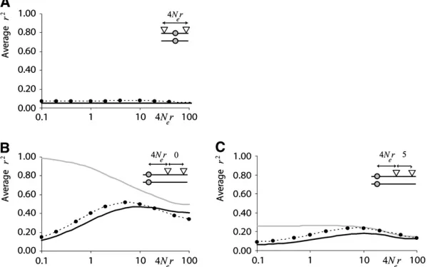
Figure5.—The effects of a selective sweep on

patterns of LD if the selected site is either sepa-rating (A) or adjacent to (B and C) the neutral loci. In each plot the shaded line indicates the prediction of Equation 6 allowing for finite sam-ple size but not for recent mutations, the solid line indicates the prediction of Equation 6 allow-ing for finite sample size and for recent muta-tions, and the solid circles and dotted line show the values obtained by fully stochastic sim-ulation. The configuration relating to each plot is shown in the top right corner (triangles, neu-tral loci; circles, selected loci). (A) The selected site is at the midpoint between the two selected loci, which are separated by the recombination fraction shown. (B) The selected site is adjacent to the neutral loci at the recombination fraction indicated beyond the proximal locus and the two neutral loci are completely linked. (C) The same as B except the two neutral loci are separated by a recombination fraction of 4Ner¼5. In all cases 106simulations were performed with a sample size of 20 and a scaled selection

coefficient of 4Ns¼400 using the SelSim package (Spencerand Coop2004).

TABLE 1

Probability of observing an incompatibility across a selective sweep

PrfH4ga _{PrfH4jMAF.10%g} 4Nerb S¼0 S¼400 S¼0 S¼400

0.1 0.0019 0.00007 0.0044 0.00062

0.2 0.0038 0.00016 0.0094 0.0012

0.4 0.0086 0.00031 0.020 0.0028

1 0.024 0.0011 0.053 0.0095

2 0.051 0.0030 0.11 0.024

4 0.098 0.0087 0.21 0.055

10 0.18 0.035 0.36 0.15

20 0.23 0.086 0.46 0.29

40 0.26 0.17 0.53 0.44

100 0.29 0.28 0.59 0.58

a

Estimated from 106_{simulations withn¼20, conditioning}

on segregation at both neutral loci. b

by the selected site is eliminated. As previously noted (Kimand Nielsen2004), there is a simple genealogical

explanation for this observation. In effect, the genea-logical interpretation of LD implies that significant LD will occur when the coalescent time for a pair of chro-mosomes at one position on a chromosome is infor-mative about the coalescent time for the same pair of chromosomes at another position (relative to the co-alescent time of all other pairs of chromosomes). Within a star-like genealogy all pairs of chromosomes coalesce at the same time. Consequently the coalescent time for a given pair at one point is uninformative about the coalescent time at any other point for the same pair (i.e., there is no variance in coalescence time within the star), and there is no LD. Moving away from the selected site recombination events will allow linked neutral sites to revert to the neutral distribution of genealogies. How-ever, such ‘‘recovery’’ from the star-like genealogy hap-pens independently on the two sides of the selected site. Consequently, the coalescent time for a pair of chro-mosomes on one side of the selected site will always be uninformative about the coalescent time for the same pair of chromosomes on the other side.

What is the implication of this result for understand-ing patterns of variation? The most obvious issue is that selective sweeps, through abolishing LD, may create patterns that look like recombination hotspots. Indeed, it has been shown that one statistical test for hotspots does have an elevated false positive rate at selective sweeps (Reedand Tishkoff2005). However, it should

be noted that the patterns of genetic variation (and underlying genealogies) associated with a hotspot and those associated with a selective sweep are strikingly dif-ferent. In humans, hotspots are typically short (1–2 kb) regions where there is a very rapid breakdown in LD, and there are many ‘‘detectable’’ recombination events and no distortion to the distribution of marginal gene-alogies (i.e., no distortion to the frequency distribution of neutral variation) ( Jeffreyset al.2001). In contrast, a

selective sweep of considerable strength will affect the

density and frequency distribution of polymorphism over considerable distances. For example, a scaled se-lection coefficient of 4Nes¼400 (a selection coefficient

of 1% in humans) will affect the frequency distribu-tion of polymorphism up to a genetic distance of at least 4Ner ¼28 on either side (this is the distance at

which there is a 50% chance of lineage escaping the sweep). In humans, the average recombination rate is

4Ner ¼0:4=kb in European populations (Myerset al.

2005), such that a region some 140 kb in size should be strongly affected. In short, even if a sweep does in-fluence LD in such a way as to resemble a hotspot, the sweep is also likely to lead to unusual patterns of vari-ation that are indicative of a selective sweep.

One way to ask the question of whether selective sweeps can create false hotspots is to ask whether, con-ditioning on seeing polymorphism at given genetic distances on either side of the selected mutation, the evidence for historical recombination is greater or less than under the neutral model. Table 1 shows how selective sweeps influence the probability of seeing all four possible haplotypes relative to the neutral case. Under the infinite-sites model such data sets are direct evidence for recombination (Hudson and Kaplan

1985). The patterns are quite striking: sweeps lead to a dramatic decrease in the probability of observing all four haplotypes relative to the neutral model. This is true whether all mutations are considered or just those .10% in frequency. In short, selective sweeps do not lead to any increase in the evidence for recombination. The reported bias to one method for detecting hotspots (Reedand Tishkoff2005) therefore is likely to result

from the fact that this method uses a nongenealogical model for patterns of variation. Analysis of data sets sim-ulated with selective sweeps indicates that coalescent-based estimators of the recombination rate show no such local increase in estimated rate. Rather, the de-pression in the opportunity for recombination at such sites also leads to a slight decrease in average estimated rate (Figure 6).

Figure6.—The effect of selective sweeps on

es-timates of the recombination rate. For data sets previously simulated with a selective sweep (the position of which is indicated by the vertical bar) and constant recombination rate (R¼ 10; indicated by the dotted line) (Reedand Tishkoff

2005), a model of variable rate recombination was fitted using the reversible-jump MCMC method of McVeanet al.(2004), using a block

penalty of 5. Four series of data sets were ana-lyzed, each of 100 replicates, with S ¼ 4Nes ¼

Selective sweeps can increase (and decrease) LD: While LD between neutral loci is eliminated by a selec-tive sweep at an intervening site, if the selected site does not separate the neutral loci LD can be increased or decreased depending on their proximity to the selected site. A further complication is that the age of the neutral mutations relative to the selected one has critical con-sequences for the magnitude of LD. If both neutral loci are closely linked to the selected site, mutations older than the selected one will typically show strong LD and younger mutations will typically have little or no LD. When both features are combined the result is a non-monotonic relationship between the proximity of a pair of neutral loci to a selected one and the strength of LD. What are the implications of these results for the interpretation of empirical patterns of genetic varia-tion? Previous work has suggested that incorporating information on LD does not greatly improve the power of statistical approaches to identifying selective sweeps (Kimand Nielsen2004). This result is understandable

given the complexity of the patterns described. One possibility is that incorporating information about the age of linked neutral polymorphism (for example, by comparison with related populations in which no sweep is thought to have occurred) may increase the power to detect selection. In particular, sweeps will lead to series of old SNPs at low frequency and in strong LD inter-leaved with series of young SNPs at low frequency and in very low LD. Of course, inferences about the age of a mutation within the population that has experienced selection will be confounded by the effect of the sweep. One argument against using patterns of LD directly to make inferences about selective sweeps is that their effects on LD can all be understood in terms of the generation of a star-like genealogy at the selected site. Consequently, the most powerful methods for detecting selective sweeps will be those that are most powerful at detecting local star-like genealogies with short times to the MRCA (Kimand Stephan2002; Kimand Nielsen

2004; Nielsen et al. 2005). For example, of existing

methods to detect recent, complete selective sweeps, perhaps the most powerful is one that compares models with and without a local star-like genealogy at a puta-tively selected site using only the allele-frequency distri-bution (Nielsenet al.2005). However, what the results

presented here show is that selective sweeps can induce unusual patterns of association between neutral muta-tions near selected sites, a feature that is currently not considered in this method. In effect, the results sug-gest that there may be additional information about selective sweeps in the way genetic variation recovers around a selected locus; however, it remains to be seen whether such recovery differs systematically from cases where star-like genealogies have occurred by chance or through population bottlenecks.

I thank Nick Barton, Alison Etheridge, Rasmus Nielsen, Jay Taylor, and two anonymous reviewers for discussion and comments on the

manuscript and Wolfgang Stephan for providing the original in-spiration for this work.

LITERATURE CITED

Barton_{, N. H., 1998 The effect of hitch-hiking on neutral} geneal-ogies. Genet. Res.72:123–133.

Braverman, J. M., R. R. Hudson, N. L. Kaplan, C. H. Langley and W. Stephan_{, 1995 The hitchhiking effect on the site} fre-quency spectrum of DNA polymorphisms. Genetics 140:783– 796.

Coop, G., and R. C. Griffiths, 2004 Ancestral inference on gene trees under selection. Theor. Popul. Biol.66:219–232. Durrett, R., and J. Schweinsberg, 2004 Approximating selective

sweeps. Theor. Popul. Biol.66:129–138.

Etheridge, A. M., P. Pfaffelhuberand A. Wakolbinger, 2006 An approximate sampling formula under genetic hitchhiking. Ann. Appl. Probab.16:685–729.

Fay, J. C., and C. I. Wu, 2000 Hitchhiking under positive Darwinian selection. Genetics155:1405–1413.

Fu, Y. X., and W. H. Li, 1993 Statistical tests of neutrality of muta-tions. Genetics133:693–709.

Hill, W. G., and A. Robertson, 1968 Linkage disequilibrium in finite populations. Theor. Appl. Genet.38:226–231.

Hudson, R. R., 1985 The sampling distribution of linkage dis-equilibrium under an infinite allele model without selection. Genetics109:611–631.

Hudson, R. R., and N. L. Kaplan, 1985 Statistical properties of the number of recombination events in the history of a sample of DNA sequences. Genetics111:147–164.

Hudson_{, R. R., K. B}ailey_{, D. S}karecky_{, J. K}wiatowski_{and F. J.} Ayala, 1994 Evidence for positive selection in the superoxide dismutase (Sod) region ofDrosophila melanogaster. Genetics136:

1329–1340.

Jeffreys_{, A. J., L. K}auppi_{and R. N}eumann_{, 2001 Intensely punctate} meiotic recombination in the class II region of the major histo-compatibility complex. Nat. Genet.29:217–222.

Kaplan_{, N. L., R. R. H}udson_{and C. H. L}angley_{, 1989 The} ‘‘hitch-hiking effect’’ revisited. Genetics123:887–899.

Kim_{, Y., and R. N}ielsen_{, 2004 Linkage disequilibrium as a signature} of selective sweeps. Genetics167:1513–1524.

Kim_{, Y., and W. S}tephan_{, 2002 Detecting a local signature of genetic} hitchhiking along a recombining chromosome. Genetics 160:

765–777.

MaynardSmith, J., and J. Haigh, 1974 The hitch-hiking effect of a favourable gene. Genet. Res.23:23–35.

Mc_Vean_{, G. A., 2002 A genealogical interpretation of linkage} disequilibrium. Genetics162:987–991.

Mc_Vean_{, G. A., S. R. M}yers_{, S. H}unt_{, P. D}eloukas_{, D. R. B}entley

et al., 2004 The fine-scale structure of recombination rate variation in the human genome. Science304:581–584. Myers, S., L. Bottolo, C. Freeman, G. McVeanand P. Donnelly,

2005 A fine-scale map of recombination rates and hotspots across the human genome. Science310:321–324.

Nielsen_{, R., S. W}illiamson_{, Y. K}im_{, M. J. H}ubisz_{, A. G. C}lark_{et al.,} 2005 Genomic scans for selective sweeps using SNP data. Genome Res.15:1566–1575.

Ohta_{, T., and M. K}imura_{, 1971 Linkage disequilibrium between} two segregating nucleotide sites under the steady flux of mu-tations in a finite population. Genetics68:571–580.

Pluzhnikov, A., and P. Donnelly, 1996 Optimal sequencing strat-egies for surveying molecular genetic diversity. Genetics 144:

1247–1262.

Przeworski_{, M., 2002 The signature of positive selection at} ran-domly chosen loci. Genetics160:1179–1189.

Reed, F. A., and S. A. Tishkoff, 2005 Positive selection can create false hotspots of recombination. Genetics172:2011–2014. Sabeti, P. C., D. E. Reich, J. M. Higgins, H. Z. Levine, D. J. Richter

et al., 2002 Detecting recent positive selection in the human genome from haplotype structure. Nature419:832–837. Song_{, Y. S., and J. S. S}ong_{, 2007 Analytic computation of the}

Spencer, C. C., and G. Coop, 2004 SelSim: a program to simulate population genetic data with natural selection and recombina-tion. Bioinformatics20:3673–3675.

Stephan_{, W., T. W}iehe_{and M. W. L}enz_{, 1992 The effect of strongly} selected substitutions on neutral polymorphism: analytical results based on diffusion theory. Theor. Popul. Biol.41:237– 254.

Stephan, W., Y. S. Songand C. H. Langley, 2006 The hitchhiking effect on linkage disequilibrium between linked neutral loci. Genetics172:2647–2663.

Strobeck, C., and K. Morgan, 1978 The effect of intragenic recom-bination on the number of alleles in a finite population. Genetics

88:829–844.

Wakeley_{, J., and S. L}essard_{, 2003 Theory of the effects of} popula-tion structure and sampling on patterns of linkage disequilib-rium applied to genomic data from humans. Genetics 164:

1043–1053.

Communicating editor: R. Nielsen

APPENDIX A

Transition probabilities when the selected mutation separates the neutral loci

Configuration at end of selection phase

Probability given starting configuration

Configuration at start of neutral phase

ðiS_jS_;iS_jS_{Þ ði}S_jS_;iS_kS_{Þ ði}S_jS_;kS_lS_Þ

ðiS_jS_;iS_jS_{Þ q}2

xq

2

y 0 0 O

ðiS_jS_;iS_kW_{Þ 2q}2

xpyqy qx2pyqy 0 O

ðiS_jW_;iS_kS_{Þ 2p}

xqxqy2 pxqxqy2 0 O

ðiS_jW_;iS_kW_{Þ 2p}

xqxpyqy pxqxpyqy 0 B

ðiS_jS_;kW_lW_{Þ q}2

xp2y qx2py2 qx2p2y O

ðiW_jW_;kS_lS_{Þ p}2

xq

2

y p

2

xq

2

y p

2

xq

2

y O

ðiS_jW_;kS_lW_{Þ 2p}

xqxpyqy 3pxqxpyqy 4pxqxpyqy B

ðiS_jW_;kW_lW_{Þ 2p}

xqxp2y 2pxqxp2y 2pxqxp2y C

ðiW_jW_;kS_lW_{Þ 2p}2

xpyqy 2px2pyqy 2px2pyqy C

ðiW_jW_;kW_lW_{Þ p}2

xp

2

y p

2

xp

2

y p

2

xp

2

y C

ðiS_jS_;iS_kS_{Þ 0 q}2

xqy2 0 O

ðiS_jS_;kS_lW_{Þ 0 q}2

xpyqy 2qx2pyqy O

ðiS_jW_;kS_lS_{Þ 0 p}

xqxqy2 2pxqxqy2 O

ðiS_jS_;kS_lS_{Þ 0 0 q}2

xqy2 O

An example of the transition probabilities for the changes in configuration that occur during the selection is given in Figure 2. Here we give the transition probabilities for the different starting configurations. For nota-tion, letðiS_jS_;iS_jS_{Þrepresent the configuration where at locusx(to the left of the selected site) the two}

chro-mosomesiandjhave been sampled and both carry the selected allele and at locusythe same two chromosomes have been sampled and again, both carry the selected allele. Using this notation,ðiS_jW_;iS_kW_{Þis, for example,}

the configuration where at locusxchromosomeicarries the selected allele and chromosomejcarries the wild type, while at locusychromosomeihas again been sampled (and therefore by necessity carries the selected allele), while a third chromosome,k, carries the wild-type allele. The transition probabilities during the selec-tion phase for each of the three starting configuraselec-tions are given below. Note thatqi¼1piand that the labels

APPENDIX B

Transition probabilities when the selected mutation is adjacent to the neutral loci

Configuration at end of selection phase

Probability given starting configuration

Configuration at start of neutral phase

ðiS_jS_;iS_jS_{Þ ði}S_jS_;iS_kS_{Þ ði}S_jS_;kS_lS_Þ

ðiS_jS_;iS_jS_{Þ q}2

xq

2

y 0 0 O

ðiS_jW_;iS_jW_{Þ 2p}

xqxqy2 0 0 A

ðiS_jS_;iS_kW_{Þ 2q}2

xpyqy qx2qy½px1pypxpy 0 O

ðiS_jW_;iS_kW_{Þ 2p}

xqxpyqy pxqxqy½px1pypxpy 0 B

ðiW_jW_;iW_jW_{Þ p}2

xq

2

y 0 0 A

ðiS_jW_;jW_kW_{Þ 2p}

xqxpyqy pxqxqy½px1pypxpy 0 B

ðiS_jS_;kW_lW_{Þ q}2

xp

2

y q

2

xpy½px1pypxpy qx2½px1pypxpy2 O

ðiS_jW_;kW_lW_{Þ 2p}

xqxpy2 2pxqxqy½px1pypxpy 2pxqx½px1pypxpy2 C

ðiW_jW_;iW_kW_{Þ 2p}2

xpyqy p2xqy½px1pypxpy 0 B

ðiW_jW_;kW_lW_{Þ p}2

xp

2

y p

2

xpy½px1pypxpy p2x½px1pypxpy

2

C

ðiS_jS_;iS_kS_{Þ 0 q}3

xq

2

y 0 O

ðiS_jW_;iS_kS_{Þ 0 p}

xqx2q

2

y 0 O

ðiS_jS_;kS_lW_{Þ 0 q}3

xpyqy 2qx3qy½px1pypxpy O

ðiS_jW_;jW_kS_{Þ 0 p}

xqx2q

2

y 0 A

ðiS_jW_;kS_lW_{Þ 0 2p}

xqx2pyqy 4pxqx2qy½px1pypxpy B

ðiW_jW_;jW_kS_{Þ 0 p}2

xqxq2y 0 B

ðiW_jW_;kS_lW_{Þ 0 p}2

xqxpyqy 2p2xqxqy½px1pypxpy C

ðiS_jW_;kS_lS_{Þ 0 0 2p}

xqx3q

2

y O

ðiW_jW_;kS_lS_{Þ 0 0 p}2

xqx2qy2 O

ðiS_jS_;kS_lS_{Þ 0 0 q}4

xq

2

y O

The transition probabilities during the selection phase for each of the three starting configurations are given. Notation is as in

appendix a. Note thatp