ABSTRACT
HOLLAR, DONNA ALYN. Predicting Preliminary Engineering Costs for Highway Projects. (Under the direction of Min Liu, William Rasdorf, and Joseph E. Hummer.)
Preliminary engineering (PE) for a highway project encompasses two efforts: planning to minimize the physical, social, and human environmental impacts of projects and engineering design to deliver the best alternative. State transportation agencies strive to manage these efforts efficiently, seeking to maximize the utilization of limited funding and workforce productivity. Managers need a feasible PE budget early in project development. The results reported herein will enable engineers and managers to develop PE budgets during the preconstruction phase of highway project development.
Typically, transportation managers establish a project’s PE budget using a percentage of estimated project construction costs disregarding other project-specific parameters. The commonly accepted rule of thumb for PE costs is 10% of estimated construction costs. This research effort sought to improved PE cost estimation methods by investigating available historical data supporting statistical analyses, developing predictive regression models forecasting projects’ PE costs, and assessing model performance through validation.
Cost data were acquired for 461 bridge projects and 188 roadway projects let for construction between 1999 and 2009 in North Carolina. Separate analyses were performed on bridges and roadways. Both project types are included in North Carolina’s State Transportation Improvement Program. Many variables applicable for bridges were not applicable or available for roadways. Analysis of the roadway data yielded a mean ratio of PE cost to estimated construction cost (the PE cost ratio) of 11.7%. Comparatively, the bridge projects exhibited a mean PE cost ratio of 27.8%, approximately 2.4 times greater than the roadway mean. Using multiple linear regression and hierarchical linear modeling, we developed prediction models to forecast the PE cost ratio of future bridge and roadway projects.
Considering the roadway database exhibited a mean PE cost ratio of 11.7%, this AAE represents a 59% relative error. Comparatively, predictive regression modeling did yield better PE cost estimates than using the commonly accepted rule of thumb, or any single parameter estimator. However, the relative error was high, in the 40% to 60% range.
Predicting Preliminary Engineering Costs for Highway Projects
by
Donna Alyn Hollar
A dissertation submitted to the Graduate Faculty of North Carolina State University
in partial fulfillment of the requirements for the degree of
Doctor of Philosophy
Civil Engineering
Raleigh, North Carolina 2011
APPROVED BY:
_______________________________ ______________________________
Min Liu, Ph.D. William Rasdorf, Ph.D., P.E.
Co-Chair of Advisory Committee Co-Chair of Advisory Committee
________________________________ ________________________________ Joseph E. Hummer, Ph.D., P.E. Brian J. Reich, Ph.D.
BIOGRAPHY
ACKNOWLEDGEMENTS
I am grateful for the financial support provided by the Department of Civil, Construction and Environmental Engineering at NCSU, the Southeastern Transportation Center, the North Carolina Department of Transportation, and East Carolina University. Each agency provided financial support at varying times throughout my long journey toward degree completion.
The North Carolina Department of Transportation was especially instrumental in the successful completion of my research by providing both project data and access to professional experts. Notably, I thank members of the Program Development Branch, the Structure Inventory and Appraisal Unit, and Schedule Management Office, and the Financial Management Division. Many NCDOT personnel positively influenced this research effort. I appreciate and acknowledge their collective efforts.
My past supervisors at East Carolina University deserve special recognition for their unwavering encouragement that helped me persevere to the end. You know who you are and I am forever grateful.
TABLE OF CONTENTS
LIST OF TABLES ... vi
LIST OF FIGURES ... viii
1.0 INTRODUCTION ... 1
1.1 Background ... 1
1.2 Preliminary Engineering (PE) Defined... 3
1.3 Significance of the Research ... 3
1.4 Research Tasks ... 4
1.5 Research Scope and Limitations ... 4
1.6 Organization of Report ... 5
2.0 LITERATURE REVIEW ... 6
2.1 NCDOT Perspective on PE Budgeting ... 6
2.2 PE Estimation Efforts for the Transportation Industry ... 8
2.2.1 Total PE as a Percentage of Construction Costs ... 8
2.2.2 Planning and Design Components of PE ... 11
2.2.3 PE Provider: In-house versus Consultant ... 12
2.3 Construction Cost Estimating for Transportation Projects ... 14
2.3.1 Estimate Development Timeline ... 14
2.3.2 Estimating Practices in the Transportation Industry ... 17
2.3.3 Research Efforts on Construction Estimating Techniques ... 18
2.3.4 NCDOT Construction Cost Estimating Practices ... 19
2.4 Applicable Statistical Analysis Techniques ... 21
2.4.1 Regression Modeling ... 21
2.4.2 Multilevel Hierarchical Modeling ... 22
2.5 Summary ... 23
3.0 BRIDGE PROJECTS: PE COST ANALYSES ... 25
3.1 Methodology ... 25
3.1.1 Bridge Database Compilation ... 26
3.1.2 Validation Sampling ... 27
3.1.3 Dependent Variable ... 28
3.2 Independent Variables for Prediction ... 30
3.2.2 Variable Correlations ... 34
3.3 Multiple Linear Regression ... 35
3.4 Hierarchical Linear Modeling ... 36
3.5 Results ... 41
3.6 Conclusions and Recommendations ... 45
4.0 ROADWAY PROJECTS: PE COST ANALYSES ... 47
4.1 Methodology ... 48
4.1.1 Roadway Database Compilation ... 48
4.1.2 Validation Sampling ... 49
4.1.3 Dependent Variable ... 49
4.2 Independent Variables for Prediction ... 51
4.3 Multiple Linear Regression ... 54
4.4 Hierarchical Linear Modeling ... 55
4.5 Results ... 60
4.6 Conclusions and Recommendations ... 63
5.0 CONCLUSIONS AND RECOMMENDATIONS ... 65
5.1 Use of Predictive Models ... 65
5.2 PE Costing Data ... 66
5.3 Extreme Instances of PE Cost Ratios ... 66
6.0 REFERENCES ... 67
APPENDICES ... 72
A. Regression Parameters for Bridge Models ... 73
B. Bridge Database ... 87
C. Regression Parameters for Roadway Models ... 144
LIST OF TABLES
Table 2.1 Findings by State Auditor Regarding Costs of NCDOT Highway Projects ... 7
Table 2.2 Estimate Classifications and Associated Accuracy Levels ... 17
Table 2.3 Listing of Innovative Techniques for Improving Construction Costs Estimates ... 19
Table 2.4 NCDOT Estimate Types and Associated Contingencies ... 21
Table 2.5 Summary Table of Relevant Research ... 24
Table 3.1 Bridge Projects Database ... 27
Table 3.2 Bridge Independent Variables Considered ... 31
Table 3.3 Categorical Variables: Influence on Cubed Root of PE Cost Ratio ... 32
Table 3.4 Numerical Variables: Correlation with Cubed Root of PE Cost Ratio ... 34
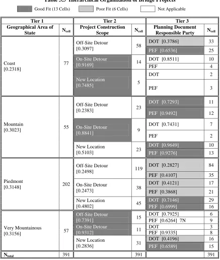
Table 3.5 Hierarchical Organization of Bridge Projects ... 40
Table 3.6 Performance of Bridge PE Cost Ratio Regression Models ... 42
Table 3.7 Bridge Reduced MLR Model Parameters ... 43
Table 3.8 Predicted PE Cost Ratio for Bridge Project B-4665... 44
Table 4.1 Roadway Projects Database ... 49
Table 4.2 Roadway Independent Variables Considered ... 52
Table 4.3 Categorical Variables: Influence on Cubed Root of PE Cost Ratio ... 53
Table 4.4 Numerical Variables: Correlation with Cubed Root of PE Cost Ratio ... 54
Table 4.5 Roadway Baseline MLR Model ... 54
Table 4.6 Hierarchical Organization of Roadway Projects ... 57
Table 4.7 Roadway Full HLM Model ... 59
Table 4.8 Performance of Roadway PE Cost Ratio Regression Models ... 61
Table 4.9 Predicted PE Cost Ratio for Roadway Project U-3601 ... 63
Table 4.10 Observed Values of Roadways’ Influential Numerical Variables ... 64
Table A.1 Bridge Full MLR Model (with interactions) ... 73
Table A.2 Reduced Bridge MLR Model (with Year of Letting Omitted) ... 74
Table A.3 Bridge HLM Model ... 75
Table A.4 Bridge HLM Model (with Surrogate) ... 79
Table A.5 Bridge HLM Model (with Mean as Surrogate) ... 83
Table A.7 Roadway Baseline MLR Model ... 144
Table A.8 Roadway Full MLR Model (with interactions) ... 144
Table A.9 Roadway Reduced MLR Model (with only numerical variables) ... 145
Table A.10 Roadway Reduced HLM Model (with 1 tier grouping) ... 145
Table A.11 Roadway Full HLM Model (with 2 tier grouping) ... 146
LIST OF FIGURES
Figure 2.1. NCDOT Transportation Program Lifecycle ... 7
Figure 2.2 DOT Reported PE Costs as a Percentage of Construction Costs ... 9
Figure 2.3 Timeline of Construction Cost Estimates for Transportation Projects ... 16
Figure 2.4 NCDOT Estimating Timeline ... 20
Figure 3.1 Distribution of PE Cost Ratio for Bridge Projects ... 29
Figure 3.2 Distribution of Cubed Root of PE Cost Ratio for Bridge Projects ... 29
Figure 3.3 Comparison of Cost Trends of Bridge Projects ... 33
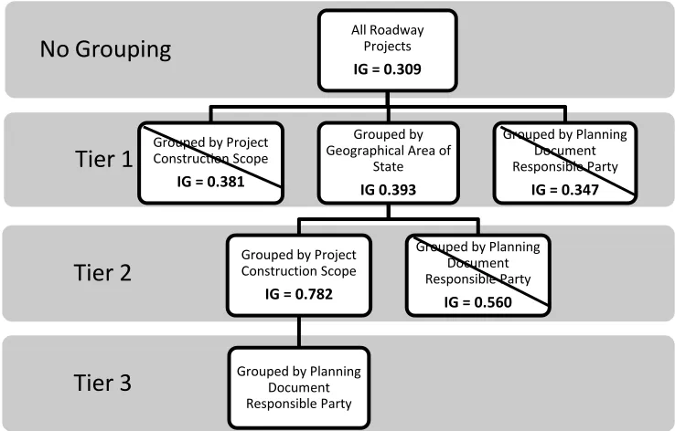
Figure 3.4 Information Gain for Bridge Hierarchical Structure ... 38
Figure 3.5 Actual versus Predicted Values for Bridge PE Cost Ratio... 45
Figure 4.1 Distributions of Cost Ratios for Roadway Projects ... 50
Figure 4.2 Information Gain for Roadway Hierarchical Structure ... 56
1.0 INTRODUCTION
This research addresses the need to accurately estimate preliminary engineering (PE) costs required to plan and design highway projects. This section discusses PE estimation history and practices. Specifically, practices at the North Carolina Department of Transportation (NCDOT) are described since NCDOT projects comprised the research dataset. The section also describes research significance, research objectives, and research scope.
1.1 Background
Over the last thirty years, transportation projects have increased in number and complexity. Accuracy of project cost estimates has become a larger concern. Initially, construction cost accountability was the focus. DOTs have adopted tighter financial controls on other project cost components such as right-of-way (ROW), utilities, mitigation, and PE costs. DOTs report cost accounting information to their governing bodies. External agencies routinely audit DOTs and investigate project costing.
Public reporting of project costs differentiates between ROW costs and construction costs. Comparisons between actual and budgeted costs are common. Similar reporting of project PE cost is increasing. Typically, PE cost estimates are based on estimated project construction costs. A search of transportation literature identified that most DOTs use a constant or sliding percentage of estimated construction costs to develop a PE budget. The most frequent percentage cited is ten percent of estimated construction costs [WSDOT 2002].
Preliminary engineering (PE) for a roadway project encompasses two efforts: planning to minimize the physical, social, and human environmental impacts of projects and engineering design to deliver the best alternative. State transportation agencies strive to manage these efforts efficiently, seeking to maximize the utilization of limited funding and workforce productivity. Managers need a feasible PE budget early in project development.
of construction cost. The survey defined PE as “the work that goes into preparing a project for construction.” The average PE cost among respondents was 10.3 percent of construction costs with a reported range of 4 to 20 percent. On a project-by-project basis, using a single, fixed-percentage estimator often results in under- or over-allocation of PE funding. This, in turn, necessitates management actions to redistribute PE funds. Avoiding such redistributions improves total project cost control and aids in reducing financial risk for current and future projects.
For NCDOT highway projects, PE costs have been a significant portion of total project costs. Consistent with other agencies, NCDOT reported PE costs of 10% of total project cost. However, there can be a wide range depending on project type and complexity. It is difficult to estimate PE costs in the early project stages since an accurate definition of project scope is unavailable. This is problematic; NCDOT is unable to plan and budget PE funds efficiently, which then affects total project cost control. It is important for NCDOT to avoid project cost escalation. One way to do so is by improving the accuracy of PE cost estimating practices.
Intuitively, factors such as project type, project complexity, project location, and PE provider influence PE costs. Previously however, no comprehensive study of factors existed, and thus, the influence of factors is theoretical. Within industry literature, there is a large body of work on cost estimation in general, but no publications specifically addressing PE cost estimation.
Shane et al. (2009) identified 18 factors related to construction cost escalation of highway projects. Through a comprehensive literature review and interviews with 20 state agencies, Shane categorized factors as either “internal” (under an agency’s control) or “external.” Key external factors attributed to cost escalation are often unknown during the early stages of project development, such as changes to design and alignment made to appease residents, business owners, or environmental interest groups [Shane et al. 2009]. As these external factors arise, they directly influence PE costs.
building construction costs noting that design phase actions influence overall construction costs. Sundaram (2008) suggests that members of the design process understand their role in overall cost containment and employ cost reduction strategies, including accurate cost estimation methods. Although Sundaram (2008) does not recommend a cost estimation model, the importance of accurate estimates is emphasized. Our work shares this emphasis.
1.2 Preliminary Engineering (PE) Defined
For this study, preliminary engineering (PE) is defined as the planning and design of a highway project for construction. PE begins when a specific highway project first receives funding authorization for planning and/or design activities. The delivery of the construction documents used for solicitation of construction contract bids (known as project letting) marks the end of PE.
Consistent with the definitions used by other investigators, PE in this study does not include right of way (ROW) acquisition or construction activities [Turochy et al. 2001; WSDOT 2002]. In general, highway projects have PE, ROW, and construction components. Costs associated with feasibility studies and/or mitigation requirements are not PE; such costs are tracked separately. PE also excludes any efforts undertaken before a specific project is identified or funding is authorized, and any efforts undertaken after a construction contract has been let.
1.3 Significance of the Research
PE costs comprise a significant portion of the total project costs. Accurate PE cost estimation can help transportation managers make the best possible programming and budgeting decisions. This research benefits managers by identifying a method to improve PE cost estimating practices. With better PE cost estimates, funding allocations can be proactive, matching the specific needs of each project.
Additionally, by having a project-specific PE cost estimate generated at the beginnning of each project’s preconstruction phase, the PE budget status becomes trackable as a performance metric.
The data collected and analyzed during this research were specific to the NCDOT. However, the research findings should prove helpful to other transportation agencies. Transportation managers in other states or other countries, could apply the methods demonstrated through this research effort to improve their own PE estimation practices.
1.4 Research Tasks
The objectives of this research were to complete a comprehensive study of the factors influencing PE costs of highway projects and to a build tool to assist transportation managers in estimating PE costs accurately and efficiently. Objectives were met through completion of the following tasks:
• Develop a comprehensive list of factors influencing PE cost.
• Conduct statistical analyses of past highway projects to identify the factors that have significant impacts on PE costs.
• Develop databases of highway projects including significant factors. • Build modeling tools for PE cost ratio estimation.
1.5 Research Scope and Limitations
The research was bounded by the scope and limitations described in this section.
The research projects utilized for this research were NCDOT Division of Highways projects selected by the following criteria:
• Projects published in North Carolina’s State Transportation Improvement Program (STIP). • Projects identified in the STIP with prefixes of B (Bridge), I (Interstate), R (Rural), or U
(Urban).
• Projects let for construction between January 1, 1999 and June 30, 2009.
1.6 Organization of Report
The acquired NCDOT data included a large portion of bridge projects (STIP prefix B) by number in comparison to roadway projects (STIP prefixes I, R, and U). Generally, bridge projects outnumbered roadway projects 3 to 1. On a cost basis, construction funding for roadways exceeded bridge funding annually. Descriptive data by project type also differed. For these reasons, this research approached PE cost analyses separately for bridge projects and roadway projects.
2.0 LITERATURE REVIEW
The author reviewed journals, agency reports, academic research studies, and NCDOT documents to assess the status of PE cost estimating practices, factors influencing PE costs, and applicable analysis techniques. A search for relevant literature found that few studies were targeted specifically at PE cost estimating for transportation projects. Knight and Fayek (2002) noted the lack of predictive models to estimate design costs when studying preconstruction project management. Prior research focused on only one phase of preconstruction such as environmental planning or technical design. In these studies, for a small sample of highway projects, factors influencing costs were identified. A number of DOTs reported PE estimating practices similar to those used by NCDOT. Some states (notably Virginia and Texas) do include PE budgets in their Statewide Transportation Improvement Program (STIP) documents. Most states report using a percentage of estimated project construction cost to establish PE budgets. Regression techniques have been implemented in construction cost estimating procedures, especially preliminary and early construction cost estimates. However, references to regression analysis applied specifically to PE cost estimating were not found.
Section 2.5 contains a summary table of the relevant research reviewed. 2.1 NCDOT Perspective on PE Budgeting
Figure 2.1 illustrates the lifecycle of a NCDOT highway project. The lifecycle involves a stair-step pattern of seven serial processes. The third and fourth process steps, project planning and project design respectively; encapsulate PE efforts as defined in this research. These processes must be completed before construction, thus PE occurs during the preconstruction phase of the project lifecycle. Preconstruction, as defined by NCDOT, begins when initial PE funding is authorized by the governing body [Merritt 2008]. A project’s preconstruction phase ends when construction contracts are let.
ROW costs and construction costs. From the 2009-2015 STIP, the amount budgeted for highway right-of-way and construction was $10.9 billion [NCDOT 2008a].
Figure 2.1. NCDOT Transportation Program Lifecycle [NCDOT 2008b]
A search for NCDOT documentation identifying specific PE budgets located the 2008 North Carolina State Auditors’ report on highway projects’ cost and schedule performance [Merritt 2008]. The State Auditor reviewed total project costs and PE, ROW, and construction cost components for 292 highway projects. Construction of audited projects was completed between April 1, 2004 and March 31, 2007. Table 2.1 contains the State Auditor’s assessment of project costs.
Table 2.1 Findings by State Auditor Regarding Costs of NCDOT Highway Projects Project Cost
Component
Estimated Costs (in millions)
Actual Costs (in millions)
PE $ 73.4 $ 117.1
ROW $ 83.8 $ 148.7
Construction $ 650.3 $ 1,020.3
Total $ 807.5 $ 1,286.1
The cost figures reported in Table 2.1 identify several cost trends:
• Actual costs exceeded estimated amounts for all cost components.
• PE expenditures increased 59 percent ($43.7 increase compared to the original $73.4 estimate).
• Actual PE expenditures represented 18 percent of estimated construction costs ($117.1 compared to $650.3).
The magnitude of the actual PE costs is of particular concern. Theoretically, if only 10.3 percent was initially budgeted (the average of PE percentages reported by WSDOT (2002)), NCDOT would have experienced insufficient PE funding to complete PE activities. This would necessitate additional hard-to-obtain PE funding authorizations and would have legislative and infrastructure management and policy implications.
2.2 PE Estimation Efforts for the Transportation Industry
PE can be broken into two components – planning and design. The planning component of PE includes all efforts required to prepare and deliver a project’s environmental documents in the preconstruction phase. In the typical project cycle, planning is initiated before design. Design PE includes all efforts required to produce the project’s construction documents. The summation of these components is a project’s total PE. All PE tasks occur in the preconstruction phase. The personnel involved in planning and design PE functions may be involved in related actions during or after construction. For example, design efforts related to construction change orders are not considered PE, but construction engineering. Similarly, environmental monitoring during construction is not PE, but construction compliance.
2.2.1 Total PE as a Percentage of Construction Costs
respondents reported that PE costs were estimated as a percentage of estimated construction costs, with percentages between five and twenty percent. Two of the nine DOTs reported using alternate techniques in certain circumstances. Texas estimates PE cost as a function of ROW width on some projects. Delaware utilizes a detailed form to guide how PE costs should be estimated based on project size. The PE cost of large projects can be estimated as a percentage of construction costs, whereas small projects should estimate required person-hours to determine PE costs. Moderate sized projects may utilize a combination of both estimating methods [Turochy et al. 2001].
As part of a comparative analysis of construction costs, Washington State DOT [WSDOT 2002] collected information from twenty-five DOTs whose members served on the AASHTO Subcommittee on Design. Survey participants were asked to identify their typical project PE cost as a percentage of construction cost. PE was defined as, “the work that goes into preparing a project for construction.” The average PE cost among respondents was 10.3 percent of construction costs and the range of costs reported was between four and twenty percent. NCDOT participated in the survey and reported PE costs of ten percent of construction costs.
Figure 2.2 summarizes geographically the PE costs acquired from the two surveys. Responses from twenty-eight DOTs were acquired and have been mapped in Figure 2.2 [Turochy et al. 2001; WSDOT 2002].
The Virginia Transportation Research Council (VTRC) assisted Virginia DOT (VDOT) during 2004 to find and implement a construction estimating tool. The estimating tool selected for statewide implementation was based on an existing spreadsheet application developed by the Fredericksburg District of VDOT. With this tool, PE costs can be estimated separately for roadways and bridges, both components of highway projects. VTRC initially derived a cost curve relating PE costs to construction costs using data from 30 completed VDOT roadway projects. The resulting ratio of PE costs to construction costs ranged from 8 to 20 percent. To adjust the cost curve for statewide use, VTRC then analyzed an additional 135 completed VDOT roadway projects. For bridges, VTRC developed a similar PE cost curve using data from 23 completed bridge projects [Kyte et al. 2004a, 2004b].
The Georgia DOT (GDOT) developed two cost estimating models. The first focused on right-of-way and utility relocation cost estimation and the second improved the planning phase construction cost estimate [Cox and Carroll 2010]. Together, both models provide an improved total project cost estimate (including PE costs) for highway projects. GDOT’s historical PE costs ranged from 6 to 12 percent of construction costs. With the new model, GDOT sets PE costs at 8 percent of the planning phase construction estimate [Cox and Carroll 2010].
consumed more internal and external resources and had longer durations when compared to other construction preplanning activities [George et al. 2008].
Schofer et al. (2010) reported on the recommendations developed during a conference organized by the Transportation Review Board and sponsored by the U.S. DOT Research and Innovative Technology Administration. The conference aimed to define essential research directions needed to manage and preserve the nation’s surface transportation infrastructure. Conference participants shared recommendations aligned into six research themes, one of which was valuation methods to support infrastructure management processes. Schofer et al. (2010) identified the need to “develop objective, quantitative, and monetary methods and models” to determine the cost required to keep the transportation system in a state of good repair.
2.2.2 Planning and Design Components of PE
Related to estimating the PE costs associated with planning, WSDOT noted in their 2002 survey that the preconstruction efforts required to meet environmental compliance requirements are highly variable between projects. Instead of asking survey respondents to quantify environmental compliance costs, WSDOT attempted to capture how these costs typically change during the preconstruction phase. Twenty-one of the twenty-five respondents (84 percent) indicated variability ranges from zero to ten percent. Three other respondents (12 percent) indicated higher variability in the eleven to twenty percent range [WSDOT 2002].
A non-linear regression model using transformations of the variables below was analyzed: • Initial planned construction cost (programmed costs)
• Complexity factors • Percent of bridges projects • Percent of roadways projects
The best-fit model was a log transformation using only one independent variable, the initial planned construction cost, to predict consultant design costs [Nassar et al. 2005]. The prediction error of the model was not reported.
Gransberg and others (2007) investigated the correlation of design fees to construction “cost growth from the initial estimate” termed CGIE. Using 31 projects of the Oklahoma Turnpike Authority (OTA), Gransberg confirmed that an inverse relationship existed between design fees and construction cost growth. Their conclusion asserted that as design fees decrease, construction cost growth (from initial estimate to final closeout) increases. Correlating design fees to design quality, the results support the premise that allocating sufficient funding in design reduces the likelihood of construction cost increases from the initial estimate. Gransberg’s measurement of cost growth from the initial estimate was a departure from other studies that measured cost growth only from the bid price. The construction cost growth (CGIE) for all projects in the study was 9.65 percent. Thus, the difference between final construction cost and the initial estimate was less than ten percent.
Gransberg’s study provided quantitative data on design costs. However, the sample size was small. Of the 31 projects investigated, 13 were roadway projects and 18 were bridge projects. The average design cost for all projects was 5.2 percent. The roadway projects design costs averaged two percent, whereas the bridge projects exhibited design costs nearly four times higher (7.6 percent). The researchers concluded “bridge design projects should command a relatively higher design fee than roadway projects due to the increased complexity of design." [Gransberg et al. 2007]
2.2.3 PE Provider: In-house versus Consultant
were greater than in-house costs. However, the magnitude of this difference varied significantly depending on the comparison methodology utilized. Wilmot et al. identified the difficulties inherent in earlier comparisons that used a similar project methodology. Though significant effort was made to identify and compare similar projects, no two projects are exactly alike.
Wilmot et al. proposed using a paired cost comparison on the same project by generating an estimated design cost to compare with the actual design cost. For in-house projects, the comparable consultant design cost would be estimated. Similarly, projects by consultants would be estimated as though completed in-house. Thus, every project compared would have two design costs, one actual and one estimated. These paired costs comparisons were analyzed using thirty-seven projects (twenty designed in-house and seventeen designed by consultants) completed between 1995 and 1997 by the Louisiana Department of Transportation and Development (LDOTD). After including cost factors such as overhead rates, space rental, and insurance in both paired costs, the overall comparison found that in-house costs are approximately 80 percent of consultants’ costs. This difference was found to be statistically significant at the 95 percent level. However, the difference was largely accounted for by the additional in-house efforts required to prepare and supervise the consultants’ contract. This supervisory effort amounted to an extra 50 hours of in-house time on average for the projects studied [Wilmot et al. 1999].
Two other incidental aspects of the Wilmot et al. study are worth noting. Using a paired cost comparison, the effect of project characteristics such as complexity, uniqueness, size, or type was eliminated. When comparing two costs for the same project, these characteristics would be equally accounted for in both cost figures. Thus, there is no way to infer how such characteristics may affect design costs. Wilmot et al. also discussed the difficulties in acquiring the necessary data from typical DOT databases. Most DOTs lack integrated databases making the data “less useful and less available.” Wilmot et al. suggests that DOTs would benefit from using “integrated client-server databases” [Wilmot et al. 1999].
the VDOT statewide estimating tool. The estimator can enter the percentage of roadway design performed by consultants and the tool automatically applies the fifty percent cost multiplier to the applicable portion of PE costs. The adequacy of the multiplier was verified using cost data from 29 consultant projects and 107 in-house projects [Kyte et al. 2004a].
The cited research of Wilmont et al. (1999) and Kyte et al. (2004a) specifically addressed design functions. Both researchers agree that consultant design costs more than in-house design. There is no literature comparing planning costs based on provider.
2.3 Construction Cost Estimating for Transportation Projects
Typically, PE costs are reported as a percentage of construction costs. Extensive research efforts to improve construction costs estimation practices have been undertaken. A full review of all such research is outside the scope of this PE estimation investigation. However, this section identifies innovative estimating techniques organized along a project timeline.
2.3.1 Estimate Development Timeline
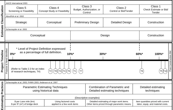
Construction estimates are prepared at multiple times within a project’s lifecycle. Few details are known at the beginning of this cycle, making accurate construction estimating difficult. The Cost Estimate Classification System developed by AACE International (2003) asserts that the degree of project definition should be “the primary characteristic to categorize estimate classes.” As a project progresses through its lifecycle, more information becomes available and the degree of project definition increases [AACE International 2003]. The additional information allows for refined construction estimates. The timeline of Figure 2.3 aims to illustrate when, along the project definition spectrum, innovative techniques could be applied.
Figure 2.3 contains three horizontal bands representing estimate classification (top), project timeline with definition levels (center), and typical estimating practices within the transportation industry (bottom).
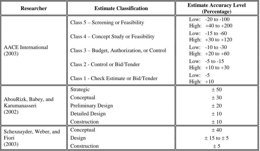
The naming convention and number of estimate classes vary between researchers. Similarly, the anticipated level of estimating accuracy for each researcher’s classification varies. Table 2.2 provides a comparative summary of the estimate classifications and corresponding accuracy levels. The multiple classification systems are included in Figure 2.3 to frame the estimating techniques identified.
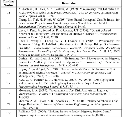
The center band of Figure 2.3 shows the level of project definition (as a percentage of total project definition) along the estimate timeline. Associating project definition levels with estimate classifications is subjective. However, for all classification schemes, project definition increases to the right along the timeline. Oval markers, labeled T1 through T10, are positioned along the timeline. Each marker represents a research technique developed to improve construction cost estimating. Table 2.3 lists each technique shown on the timeline. The position of the marker along the timeline addresses the quantity and quality of input information needed for each technique. All techniques aim to improve the accuracy of construction estimates. Section 2.3.3 provides further details on the techniques identified.
Figure 2.3 Timeline of Construction Cost Estimates for Transportation Projects
(Refer to Table 2.1 for indexof research techniques, T#) T2
Parametric Estimating Techniques using historical data
$ per Lane mile (km) $ per ft2 (m2) of bridge deck
Using factored costs applied to a few work items
Combination of Parametric and Detailed estimating techniques
Detailed estimating techniques
Detailed estimating of major work items. Other items priced through parametric means.
Item quantities priced with current labor, equip, and material costs. Schexnayder et al. 2003; FHWA 2003; Anderson et al. 2007
E s ti m a te C la s s if ic a ti o n P ro je c t T im e li n e E s ti m a ti n g P ra c ti c e s Class 5 Screening or Feasibility
Class 4
Concept Study or Feasibility
Class 3 Budget, Authorization, or
Control
Class 2 Control or Bid/Tender
Class 1 Check Estimate or Bid/
Tender AACE International 2003
Conceptual Design Construction
Schexnayder et al. 2003
Strategic Conceptual Preliminary Design Detailed Design Construction
AbouRizk et al. 2002
0%* 30%* 100%*
T8 T3 T1 T7 T9 T5T10
(Descriptive examples) T4 T6
60%* 10%*
* Level of Project Definition expressed as a percentage of full definition.
P u rp o s e & N e e d I d e n ti fi e d P o s t C o n s tr u c ti o n B id
Table 2.2 Estimate Classifications and Associated Accuracy Levels
Researcher Estimate Classification Estimate Accuracy Level
(Percentage)
AACE International (2003)
Class 5 – Screening or Feasibility Low: -20 to -100 High: +40 to +200
Class 4 – Concept Study or Feasibility Low: -15 to -60 High: +30 to +120
Class 3 – Budget, Authorization, or Control Low: -10 to -30 High: +20 to +60
Class 2 - Control or Bid/Tender Low: -5 to -15 High: +10 to +30
Class 1 - Check Estimate or Bid/Tender Low: -5 High: +10
AbouRizk, Babey, and Karumanasseri (2002)
Strategic ± 50
Conceptual ± 30
Preliminary Design ± 20
Detailed Design ± 10
Construction ± 10
Schexnayder, Weber, and Fiori
(2003)
Conceptual ± 40
Design ± 15 to ± 5
Construction ± 5
2.3.2 Estimating Practices in the Transportation Industry
DOT personnel perform project estimating for most highway projects. Approximately half of the DOTs organize their estimators into a unit dedicated to estimating. Others accomplish estimating tasks using personnel assigned to design or contract administration units. In two-thirds of the DOTs, estimators have a minimum of ten years of experience. In 42 states where external consultants prepare cost estimates, DOT personnel review those estimates in detail [Schexnayder et al. 2003].
DOTs use three general approaches to estimating [FHWA 2003, Schexnayder et al. 2003]: • Parametric estimating using historical cost figures.
• Detailed estimating using quantity takeoff techniques and pricing of labor, equipment, and materials.
• A combination of parametric and detailed techniques.
The level of project definition, as referenced along the estimating timeline, influences which estimating approach is used. Parametric estimating can be used when scoping information is very limited (project definition level is less than 5 percent). For example, if only location, length, and number of lanes are known, parametric estimating is effective [Anderson et al. 2007]. Parametric estimates rely on historical cost databases and defined relationships between cost items. Many DOTs use Trns*port, an AASHTO sponsored software package [FHWA 2003]. Trns*port’s Cost Estimating System module streamlines parametric estimating [Anderson et al. 2007]. When projects are fully scoped and detail design efforts are underway (project definition level exceeds 50 percent), detailed estimating techniques are commonly used. Detail estimating of scope line items use quantity takeoffs with material, labor, and equipment pricing. Schexnayder et al. (2003) found DOTs performing detailed estimates do so only for the major work items that account for 65 to 80 percent of project costs. The remaining work items are estimated using parametric tools [Schexnayder et al. 2003].
2.3.3 Research Efforts on Construction Estimating Techniques
Table 2.3 Listing of Innovative Techniques for Improving Construction Costs Estimates
Timeline
Marker Researcher
T1
Al-Tabtabai, H., Alex, A. P., Tantash, M. (1999). “Preliminary Cost Estimation of Highway Construction using Neural Networks.” Cost Engineering (Morgantown, West Virginia), 41(3), 19-24.
T2
Cheng, M., Tsai, H., Hsieh, W. (2008) “Web-Based Conceptual Cost Estimates for Construction Projects using Evolutionary Fuzzy Neural Inference Model.”
Automation in Construction, In Press, Corrected Proof.
T3
Chou, J., Peng, M., Persad, K. R., O'Connor, J. T. (2006). “Quantity-Based Approach to Preliminary Cost Estimates for Highway Projects.” Transportation Research Record, (1946), 22-30.
T4
Chou, J., Wang, L., Chong, W. K., O'Connor, J. T. (2005). “Preliminary Cost Estimates Using Probabilistic Simulation for Highway Bridge Replacement Projects.” Proceedings, Construction Research Congress 2005: Broadening Perspectives - Proceedings of the Congress, San Diego, CA. April 5-7, 2005. American Society of Civil Engineers, 939-948.
T5
Gkritza, K., and Labi, S. (2008). “Estimating Cost Discrepancies in Highway Contracts: Multistep Econometric Approach.” Journal of Construction Engineering and Management, 134(12), 953-962.
T6
Hegazy, T., and Ayed, A. (1998). “Neural Network Model for Parametric Cost Estimation of Highway Projects.” Journal of Construction Engineering and Management, 124(3), p. 210-218.
T7
Kyte, C. A., Perfater, M. A., Haynes, S., Lee, H. W. (2004). “Developing and Validating a Tool to Estimate Highway Construction Project Costs.”
Transportation Research Record, (1885), 35-41.
T8
Molenaar, K. R. (2005). “Programmatic Cost Risk Analysis for Highway Megaprojects.” Journal of Construction Engineering and Management, 131(3), 343-353.
T9
Shaheen, A. A., Fayek, A. R., AbouRizk, S. M. (2007). “Fuzzy Numbers in Cost Range Estimating.” Journal of Construction Engineering and Management, 133(4), 325-334.
T10 Williams, T. P. (2005). “Bidding Ratios to Predict Highway Project Costs.”
Engineering, Construction and Architectural Management, 12(1), 38-51.
2.3.4 NCDOT Construction Cost Estimating Practices
Concurrence points are defined by NCDOT (2008c) as: • CP1 Purpose and need, and study area defined • CP2 Detailed study alternatives carried forward • CP2A Bridging decisions and alignment review
• CP3 Least environmentally damaging preferred alternative (LEDPA) selection • CP4A Avoidance and mitigation
• CP4B Thirty percent hydraulic review • CP4C Permit drawings review
Figure 2.4 NCDOT Estimating Timeline
NCDOT prepares five types of construction cost estimates throughout the project’s development [Lane et al. 2008]. The oval markers positioned below the estimate timeline correlate estimate type with concurrence points and project definition level. NCDOT utilizes a detailed estimating technique for major work elements when preparing estimates. As project definition increases, the uncertainty in major work items decreases. Thus, each estimate type has different contingency percentages to account for uncertainty in the roadway work items and the structure work items. Table 2.4 summarizes these contingency rates for the five estimate types. NCDOT construction estimates are generally within five percent of bid amounts [Lane et al. 2008].
N C D O T T im e li n e 30%* At ROW
* Level of Project Definition expressed as a percentage of full definition.
N e e d & P u rp o s e I d e n ti fi e d P o s t C o n s tr u c ti o n B id C la s s if ic a ti o n CP1 Feasibility
CP2 CP2A CP3 CP4A CP4B
Functional Preliminary Preliminary Preliminary Final Prelim
0%* 60%* 100%*
Preliminary
CP4C LET
Strategic Conceptual Preliminary Design Detailed Design Construction AbouRizk et al. 2002
Type CP#
Concurrence Point Milestone NCDOT Estimate Description
Table 2.4 NCDOT Estimate Types and Associated Contingencies [Lane et al. 2008]
Construction Estimate Description
Contingency Applied to Roadway Portion
Contingency Applied to Structure Portion
Feasibility +55% +15%
Functional +45% +15%
Preliminary +35% +10%
At ROW +25% +10%
Final Preliminary +15% +5%
2.4 Applicable Statistical Analysis Techniques
Literature related to applications of multiple linear regression and hierarchical linear models is reviewed in the following section.
2.4.1 Regression Modeling
Regression techniques have often been used to predict construction-related costs. Lowe et al. (2006) utilized multiple linear regression to predict the building construction costs using data from 286 buildings constructed in the United Kingdom. The authors aimed for a predictive model that users could employ during the early stages of construction cost estimation before the detailed design has been completed. Lowe et al. identified 41 possible input variables for use in the regression model, categorized as either strategic, site related, or design. Lowe et al. concluded that the linear drivers of cost were predominately design specific. The coefficient of determination (R2) and mean absolute percentage error (MAPE) was used to judge model performance. Lowe et al. reported that their model yielded a R2 of 0.928 and a MAPE of 19.3 percent for predicting the cost of building construction but that the predictive model resulted in underestimation of very expensive projects and overestimation of very inexpensive projects.
concluded that the building projects analyzed tended to finish nearly on schedule, but over budget. Using four variables (job type, project area, project budgeted cost, planned duration) Abu Hammad et al. utilized regression techniques to find that project budgeted cost was the only significant variable in predicting final project cost, thereby concluding that the contractor was the primary driver of project cost due to underbidding practices and use of change orders. Using the same four variables, Abu Hammad et al. also predicted project duration through regression, finding that planned duration was the only significant variable on predicted duration, concluding that project duration performance is driven by the owner and engineer based on their selected contract duration and project delivery system. The regression models achieved R2 values of 99.9% for cost prediction and 93.6% for duration prediction with prediction error of -0.119 percent for cost and -0.021 for duration respectively [Abu Hammad et al. 2010].
Odeck (2003) used nonlinear multiple regression to identify project factors associated with construction cost overruns for 620 Norwegian road projects. Odeck sought to determine if cost overruns depended on the magnitude of the project cost, project delay, and/or project duration. Odeck’s regression model explained about 20 percent of the variation in cost overruns (adjusted R2 value of 0.21). Other project factors, not identified in the regression model, likely influenced the variation in cost overruns. From his model’s partial regression coefficients, Odeck concluded that estimated cost overruns decreased with increased project costs, increased with increased project duration up to a point and then decreased, and varied with geographic region. Odeck concluded that cost overruns were more predominate among smaller road projects.
2.4.2 Multilevel Hierarchical Modeling
since the power of the model is largely unaffected by the number of units in the lower or lowest level [Snijders 2005].
Steenbergen and Jones (2002) state that the goal of multilevel analysis to account for variance in a dependent variable that is measured in the lower level of analysis by considering the information from all levels of analysis. Doing so allows researchers to combine multiple levels into a single comprehensive model. Multiple levels of analysis allow the model to be more specific than a single level model. Multilevel models also allow checking of cross level interactions and make it possible to determine whether causal variables are singular or vary within the levels. Multilevel models allow for better comparative studies dealing specifically with different time periods or variables of different time periods. As mentioned in previous studies carried out by Geddes (1990) and King et al. (1994), case selection problems that are a bane to comparative research can be overcome by the use of multilevel models since the causal heterogeneity can be determined.
2.5 Summary
Table 2.5 Summary Table of Relevant Research
Researcher (Sample Size) [Industry]
Cost Focus Model Factor
Selection
Findings Significant to Proposed Research
PE R ight of W ay C ons tr uc ti on L in ear No n -L in ear F o rw ard B ack w ar d S te p w is e
AbouRizk et al. 2002
(n=213) [Infrastructure]
Accuracy of estimates was determined at 4 stages of projects’ life cycle.
Gransberg et al. 2007
(n=31) [Transportation]
Design costs inversely related to construction cost growth. Average construction cost growth = 9.65%. Design costs as percent of construction cost: Roads-2%; Bridges-7.6% Kyte et al. 2004a, 2004b
(nroads=135; nbridges = 23)
[Transportation]
PE range 8-20% of construction costs for roads. PE costs inversely related to construction costs. Consultant design
costs = 1.5(In-house design costs). Lowe et al. 2006
(n=286) [Buildings]
Log transformation of cost used. Key drivers of cost are design specific.
Nassar et al. 2005
(n=59) [Transportation] Log transformation of cost used.
Odeck 2003
(n=620) [Transportation]
Cost overruns are inversely related to project cost. Overruns are more predominate in smaller projects.
Turochy et al. 2001
(n=9) [Transportation] PE range 5-20% of construction costs
Wilmont et al. 1999
(n=37) [Transportation] In-house design costs = 80% (consultant costs). WSDOT 2002
(n=25) [Transportation]
3.0 BRIDGE PROJECTS: PE COST ANALYSES
Infrastructure funding is currently a subject of significant debate and disagreement. Funding for our future infrastructure is critical. One component of that infrastructure is bridges. As the Nation’s infrastructure ages, replacement of bridges will occur. The collapse of the MN I-35W Mississippi River Bridge [Saulny and Steinhauer 2007] highlighted the need to do so in a timely manner. This chapter looks at one of the costs of bridge projects – the cost of doing the preliminary engineering (PE) work.
Typically, PE costs are determined as a percentage of construction costs disregarding other project-specific parameters. By analyzing 461 NCDOT bridge projects let between 2001 through 2009, the research team developed statistical models linking variation in PE costs with distinctive project parameters. Modeling strategies included multiple linear regression (MLR) and hierarchical linear models (HLM). Through correlation analyses and ANOVA, twenty-eight independent variables were identified. Project parameters represented by independent variables included project scope classification (widening or new location); dimensional variables (project length, structure length, detour length, and number of spans); geographic region; and estimated costs for construction and right of way. Mean absolute percentage error (MAPE) was used to rank predictive performance when each candidate model was applied to a validation set.
These models found that bridge projects exhibited a mean PE cost ratio of 28%. This result is significantly higher than the 10.3% typically reported as the national average [WSDOT 2002]. However, the reported average did not distinguish between project type – bridges or roadways. This chapter investigates data sources, develops a model to predict PE cost, and assesses the performance of the model.
3.1 Methodology
3.1.1 Bridge Database Compilation
The research team obtained project descriptive data, cost estimates, and actual cost expenditures for bridge projects let for construction from NCDOT. The project identification number established in the STIP served as the key field linking all data sources and identifying all projects. Because preconstruction project data are housed in several independent databases maintained by different NCDOT units data collection required a significant effort.
The ten data sources used to populate the bridge project database are listed below.
1. Online Bid Tabulations & Annual Bid Averages Summary
2. Pre-2002 Project Management Data System (obsolete mainframe system) 3. Post-2002 Project Management Data System (SAP based)
4. 12-Month Projected Letting List
5. National Bridge Inventory System Data (NBIS) 6. State Transportation Improvement Plan (STIP)
7. Trns*port© Program Modification - Project Type Coding 8. Online Construction Plans
9. Board of Transportation Minutes and Funding Authorizations 10. North Carolina State Publications Clearinghouse
We accessed NCDOT’s online Bid Tabulations and Annual Bid Averages Summary to create our own study database of bridge projects let for construction during January 1, 2001 through June 30, 2009. We queried NCDOT’s project management systems to acquire actual PE costs. Projects having complete letting data and PE cost data were considered candidate projects for the bridge database. We used the additional seven data sources to fully populate the database for each candidate project. NCDOT’s data for the National Bridge Inventory System (NBIS) provided values for fourteen independent variables. The data set yielded 461 bridges for which sufficient data was available for all variables. The bridge database is detailed in Appendix B, Table A.6.
clearance, located in rural areas crossing water features. Rehabilitation of existing bridges outnumbered new location projects by three to one. The typical design was a concrete cast in place structure with three main spans on average. The mean construction cost was $1.2 million with a median cost of $910 thousand.
The ratio of actual PE costs to estimated STIP construction costs was selected as the dependent variable for cost regression analyses for all 461 bridge projects. This ratio is referred to as the project’s PE cost ratio. Using a cost ratio rather than actual cost values allowed modeling across all levels of construction costs and eliminated conversion of cost values to a common base year to account for inflation. Each project’s PE costs and estimated STIP construction costs were assumed to be from the same time period.
Column 3 of Table 3.1 displays the mean PE cost ratio for bridge projects let each calendar year. The total mean PE cost ratio for the 461 projects was 27.8 percent. The 95th percent confidence interval (CI) for total mean PE cost ratio was 26.0 to 29.6 percent. The PE cost ratio among the 461 bridge projects varied widely, ranging from 0.8 percent to 152 percent of estimated construction costs.
Table 3.1 Bridge Projects Database
Calendar Year of Letting
Number of Bridge Projects
Mean PE Cost Ratio
2001 44 25.6%
2002 62 27.7%
2003 50 25.6%
2004 69 20.9%
2005 48 20.0%
2006 31 9.2%
2007 43 47.1%
2008 98 31.4%
2009 (Jan – Jun) 16 40.3%
Total 461 27.8%
3.1.2 Validation Sampling
Each candidate regression model predicted the response variable. The prediction was then compared to the actual value associated with each validation project. This comparison quantified prediction error indicating bias in the model’s prediction capability. Bias is the tendency of a model to systematically under- or over-predict the response variable. The average absolute error (AAE) and mean absolute percent error (MAPE) were used to quantify prediction precision. A model with lower values in both bias and precision is preferred over another candidate model [Sheiner and Beal 1981]. 3.1.3 Dependent Variable
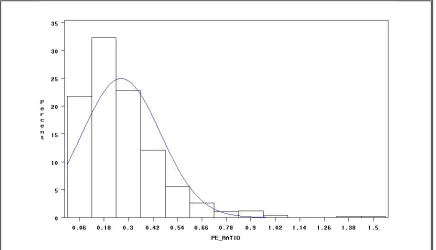
A project’s PE cost ratio is the ratio of actual PE cost to the estimated STIP construction cost. We calculated this ratio for all 461 bridge projects and investigated the distribution of PE cost ratio values. Figure 3.1 shows these results. The horizontal axis of Figure 3.1 reflects the range of actual PE cost ratio values which range from a minimum of 0.008 (0.8%) to a maximum of 1.522 (152%). The vertical axis indicates the number of projects (as a percentage of the total 461 projects) exhibiting a PE cost ratio within a 0.12 range along the x-axis. Figure 3.1 shows that the PE cost ratio distribution for the 461 bridge projects is left-skewed, exhibiting a non-normal shape.
Figure 3.1 Distribution of PE Cost Ratio for Bridge Projects
Since a power transformation was applied to normalize the response variable (cubed root of PE cost ratio), a back transformation is necessary to report prediction results in terms of the original response variable (PE cost ratio). Equations 1, 2, and 3 [Taylor 1986] describes the back transformation computation for the cubed root transformation.
[Eq. 1] Estimated Median Response = (Predicted Cubed Root of Response)3
[Eq. 2] Transformation Correction Factor = 1 +
(
(variance)(1 - ⅓))
2(Pred. Cubed Root of Response)2[Eq. 3] Estimated Mean Response = (Est. Median Response)(Transf. Corr. Factor)
Applying this back transformation requires the variance of the predicted response variable. The variance was 0.0229 for the bridge database.
3.2 Independent Variables for Prediction
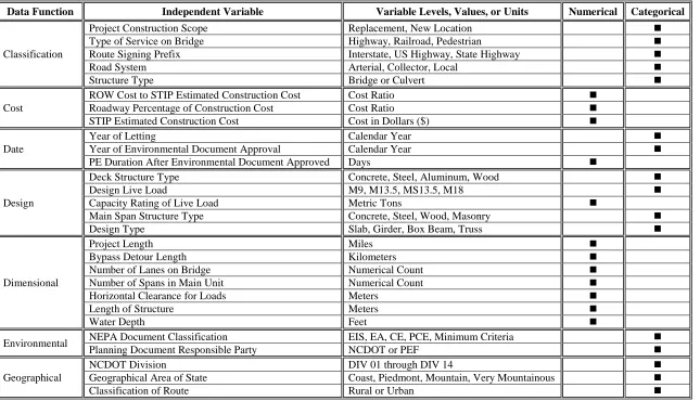
Prior to analysis, the acquired data for all bridge projects were grouped by data function: classification, cost, date, design, dimensional, environmental, and geographical. Correlation and sensitivity analyses followed to assess statistically each candidate variable, resulting in identification of 28 independent variables. These 28 variables describe project-specific parameters. Table 3.2 lists the 28 independent variables used in model development. Twelve of the 28 are numerical. The remaining 16 are categorical.
Table 3.2 Bridge Independent Variables Considered
Data Function Independent Variable Variable Levels, Values, or Units Numerical Categorical
Classification
Project Construction Scope Replacement, New Location
Type of Service on Bridge Highway, Railroad, Pedestrian
Route Signing Prefix Interstate, US Highway, State Highway
Road System Arterial, Collector, Local
Structure Type Bridge or Culvert
Cost
ROW Cost to STIP Estimated Construction Cost Cost Ratio
Roadway Percentage of Construction Cost Cost Ratio
STIP Estimated Construction Cost Cost in Dollars ($)
Date
Year of Letting Calendar Year
Year of Environmental Document Approval Calendar Year
PE Duration After Environmental Document Approved Days
Design
Deck Structure Type Concrete, Steel, Aluminum, Wood
Design Live Load M9, M13.5, MS13.5, M18
Capacity Rating of Live Load Metric Tons
Main Span Structure Type Concrete, Steel, Wood, Masonry
Design Type Slab, Girder, Box Beam, Truss
Dimensional
Project Length Miles
Bypass Detour Length Kilometers
Number of Lanes on Bridge Numerical Count
Number of Spans in Main Unit Numerical Count
Horizontal Clearance for Loads Meters
Length of Structure Meters
Water Depth Feet
Environmental NEPA Document Classification EIS, EA, CE, PCE, Minimum Criteria
Planning Document Responsible Party NCDOT or PEF
Geographical
NCDOT Division DIV 01 through DIV 14
Geographical Area of State Coast, Piedmont, Mountain, Very Mountainous
3.2.1 Variable Sensitivity
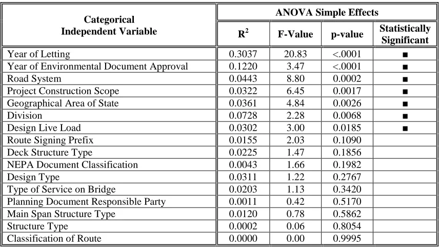
For each of the 16 categorical variables, we performed a one-way ANOVA to determine if differences between levels were significant. ANOVA also provided the coefficient of determination (R2) explaining the proportion of the variation in the response variable explained by changes in each independent, categorical variable. This is comparable to simple linear regression between two variables when the levels of all other independent variables are held constant.
Table 3.3 displays the ANOVA results for the 16 categorical variables including R2, F-value, and p-values. The p-values were used to identify the categorical variables having statistically significant differences in project values assigned for each categorical variable. Bullets in the right column indicate the seven variables with significant differences in levels. Among these seven, the R2 values were reviewed to determine the level of influence each variable had on the cubed root of PE cost ratio when all other variables are held constant. The R2 values range from 0.03 to 0.30. The two variables having the largest R2 values were date related: year of letting and year of environmental document approval. The other five variables exhibited considerably lower R2 values.
Table 3.3 Categorical Variables: Influence on Cubed Root of PE Cost Ratio
Categorical Independent Variable
ANOVA Simple Effects
R2 F-Value p-value Statistically
Significant
Year of Letting 0.3037 20.83 <.0001 ■
Year of Environmental Document Approval 0.1220 3.47 <.0001 ■
Road System 0.0443 8.80 0.0002 ■
Project Construction Scope 0.0322 6.45 0.0017 ■
Geographical Area of State 0.0361 4.84 0.0026 ■
Division 0.0728 2.28 0.0068 ■
Design Live Load 0.0302 3.00 0.0185 ■
Route Signing Prefix 0.0155 2.03 0.1090
Deck Structure Type 0.0225 1.47 0.1856
NEPA Document Classification 0.0043 1.66 0.1982
Design Type 0.0311 1.22 0.2767
Type of Service on Bridge 0.0203 1.13 0.3420
Planning Document Responsible Party 0.0011 0.42 0.5170
Main Span Structure Type 0.0120 0.78 0.5862
Structure Type 0.0002 0.06 0.8054
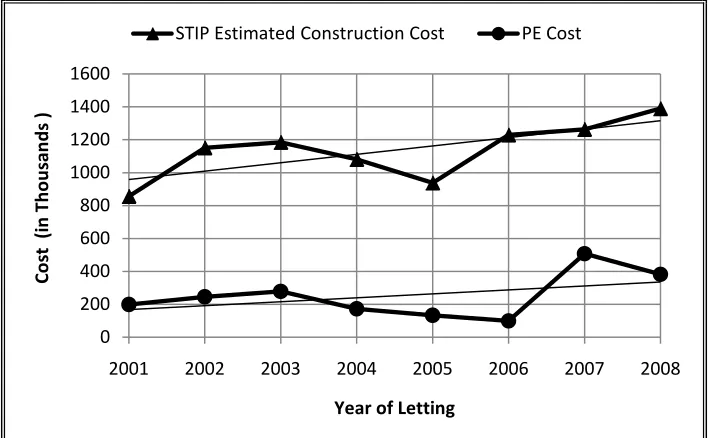
The initial expectation was that the year of letting would aid in project identification only. From an investigation of cost trends between 2001 and 2008, we discovered that both STIP estimated construction costs and PE costs exhibited a positively sloped trend line. Figure 3.3 displays this finding; STIP estimated construction costs are graphed on the upper line and PE costs are graphed on the lower line. The characteristic of both costs are similar except for the year 2006. PE costs continued to decrease between 2005 and 2006 when construction costs began increasing; then PE costs increased sharply in 2007.
The comparative change in PE costs between 2006 and 2007 does not match the comparative change in STIP estimated construction costs for the same time period. Unfortunately, discussions with NCDOT personnel did not aid in discovering the cause of this anomaly. No changes in design standards, environmental regulations, or administrative processes could be linked to the sharp PE cost increase. We hypothesized that any longitudinal trend in PE costs would mirror the longitudinal trend in construction costs. Under this assumption, date-based variables with historical levels would not be effective predictor variables during future time periods. There would be no meaningful way to assign past dates (such as year of letting) to represent a future trend. Therefore, the three variables designated in Table 3.2 as date related were rejected as predictor variables.
Figure 3.3 Comparison of Cost Trends of Bridge Projects 0
200 400 600 800 1000 1200 1400 1600
2001 2002 2003 2004 2005 2006 2007 2008
Co
st
(
in
T
ho
us
an
ds
)
Year of Letting
3.2.2 Variable Correlations
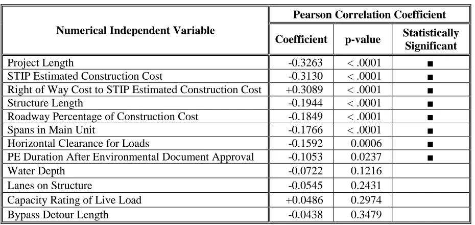
For numerical variables, correlation coefficients indicate the degree of linear association between variables. Correlation coefficients for the 12 numerical independent variables and the response variable are provided in Table 3.4. Correlation coefficients can range from -1 to +1. Larger coefficient values, either positive or negative, indicate a stronger linear association between variables. Coefficient values of zero indicate no linear association between variables. Positive coefficients indicate that the independent variable and response variable move together (positive sloped line); negative coefficients indicate the independent variable and response variable move in opposite directions (negative sloped line).
Table 3.4 reports the Pearson correlation coefficient and accompanying p-value for each numerical variable. Eight statistically significant variables (based on p-values) are indicated by bullet entries in the right column. For these eight variables, the coefficient values range from 0.10 to 0.30 indicating a weak linear association with the response variable. The three variables with highest coefficients are project length, STIP estimated construction cost, and right of way cost to STIP estimated construction cost with values of -0.33, -0.31, and +0.31 respectively.
Table 3.4 Numerical Variables: Correlation with Cubed Root of PE Cost Ratio
Numerical Independent Variable
Pearson Correlation Coefficient
Coefficient p-value Statistically Significant
Project Length -0.3263 < .0001 ■
STIP Estimated Construction Cost -0.3130 < .0001 ■
Right of Way Cost to STIP Estimated Construction Cost +0.3089 < .0001 ■
Structure Length -0.1944 < .0001 ■
Roadway Percentage of Construction Cost -0.1849 < .0001 ■
Spans in Main Unit -0.1766 < .0001 ■
Horizontal Clearance for Loads -0.1592 0.0006 ■
PE Duration After Environmental Document Approval -0.1053 0.0237 ■
Water Depth -0.0722 0.1216
Lanes on Structure -0.0545 0.2431
Capacity Rating of Live Load +0.0486 0.2974
The project team also determined the correlations between independent numerical variables. This analysis identified the independent variables that were linearly related to each other and would perform the same function in the regression model. For example, lanes on structure and horizontal clearance for loads have a Pearson correlation coefficient of 0.597. Only one of the two variables should be used in a regression model, since there is a moderately high linear association between the two variables. Table 3.4 shows the linear relationship between lanes on structure and the response variable to be statistically insignificant, while the correlation coefficient for horizontal clearance for loads and the response variable is significant. Horizontal clearance for loads is the better independent variable for model building.
3.3 Multiple Linear Regression
Selecting the “best” model using multiple linear regression (MLR) can be difficult if there are a large number of independent variables. Common variable selection techniques involve forward-, backward-, and stepwise-selection methods. To assist in model selection, we utilized the GLMSLECT procedure within the SAS statistical software package. In addition to forward-, backward-, and stepwise-selection, GLMSELECT provides two additional variable selection methods: least angle regression (LAR) and least absolute shrinkage and selector operator (LASSO). The GLMSELECT procedure provides an efficient starting point for model selection. Model refinement can then follow using intuitive insights gained from data familiarity [Cohen 2006].
Recall that the bridge database was divided into a modeling set (391 projects) and a validation set (70 projects). The modeling set was used for constructing regression models.
We considered both numerical and categorical variables when utilizing the GLMSELECT procedure for variable selection. Initially, all seven categorical variables identified as statistically significant in Table 3.3 were considered. Based on input from NCDOT staff, two environmental variables continued to hold interest and were included even though Table 3.3 reports both as statistically insignificant: NEPA document classification and planning document responsible party.
GLMSELECT iterations to assess model fit. The best MLR model achieved an adjusted R2 of 0.698 utilizing five categorical and three numerical variables with first level interactions. Appendix Table A.1 displays the complete regression parameters for the intercept, each significant variable, and each significant interaction for the full model. However, this full model MLR contained the year of letting as a predictor variable. Since we rejected all date-related variables as predictors, the GLMSELECT procedure was repeated with year of letting omitted as a candidate variable.
The reduced MLR model selected achieved an adjusted R2 of 0.2745 utilizing eight variables: four numerical (N) and four categorical (C) with first level interactions between variables. The selected variables are listed below:
• Right of Way Cost to STIP Estimated Construction Cost (N) • Roadway Percentage of Construction Cost (N)
• STIP Estimated Construction Cost (N) • Bypass Detour Length (N)
• Project Construction Scope (C) • NCDOT Division (C)
• Geographical Area of State (C)
• Planning Document Responsible Party (C)
Table 3.7 (presented in of the Results section of this chapter) lists all the regression parameters for the reduced MLR model.
3.4 Hierarchical Linear Modeling