Development of a regression model to predict preliminary engineering costs

(1)

Development of a Regression Model to Predict Preliminary

Engineering Costs

Donna Hollar, Ingrid Arocho, Joseph Hummer, Min Liu, William Rasdorf

Preliminary engineering (PE) for a highway project encompasses two efforts: planning to minimize the physical, social, and human environmental impacts of projects and engineering design to deliver the best solution. PE efforts begin years in advance of the project’s actual construction operations, often five years or more. An efficient and accurate method to estimate PE costs would benefit transportation departments by facilitating funding allocation projections. Lacking an effective tool to estimate PE cost based on project characteristics, departments of transportation typically estimate PE costs as a fixed percentage of estimated construction costs disregarding other project-specific parameters.

By analyzing 505 North Carolina Department of Transportation (NCDOT) bridge projects awarded for construction from 1999 through 2008, a multiple linear regression model was developed to link variation in PE costs to a set of distinctive project data. Published bid summaries, bridge inventory and assessment reports, NCDOT’s project management system, and published environmental reports were used as sources of project data. The model explained approximately 60 percent of the PE cost variation between projects. Results indicate that right-of-way costs, regional location, and scope delineators are among the project-specific parameters that most influence PE costs of bridge projects. By considering numerous parameters (expressed as independent variables) a more accurate prediction for future projects’ PE costs can be developed.

INTRODUCTION

For this study, preliminary engineering (PE) is defined as the planning and design of a highway project for construction. PE begins when a specific highway project first receives funding authorization for planning and/or design activities. The delivery of the construction documents used for solicitation of construction contract bids (known as project letting) marks the end of PE. Consistent with other investigators’ definitions, PE in this study does not include right of way (ROW) acquisition or construction activities [Turochy et al. 2001; WSDOT 2002].

In stark contrast to the amount of research aimed at improving construction estimates, minimal research directed at PE estimation, especially in the transportation field, exists. Investigators Knight and Fayek (2002) noted the lack of predictive tools to estimate design costs when studying preconstruction project management.

(2)

responsibility through improved budgeting and accounting accuracy. PE costs comprise a significant portion (on the order of 10 percent) of total project costs, but current budgeting processes often do not consider the unique characteristics of each project.

PE estimates are frequently based on estimated project construction costs. As part of a comparative analysis of construction costs, Washington State DOT [WSDOT 2002] collected information from twenty-five DOTs whose members served on the AASHTO Subcommittee on Design. Survey participants were asked to identify their typical project PE cost as a percentage of construction cost. PE was defined as “the work that goes into preparing a project for construction.” The average PE cost among respondents was 10.3 percent of construction costs and the range of costs reported was between 4 and 20 percent. This study indicates that continuing to estimate PE costs using a fixed percentage method is inefficient over the project cycle. On a project by project basis, this results in under-allocation or over-allocation of PE funding, which, in turn, necessitates management actions to redistribute PE funds. Avoiding such redistributions improves total project cost control and aids in reducing financial risk for current and future projects.

The Virginia Transportation Research Council (VTRC) assisted Virginia DOT (VDOT) during 2004 to find and implement a construction estimating tool. The estimating tool selected for statewide implementation was based on an existing spreadsheet application developed by the Fredericksburg District of VDOT. With this tool, PE costs can be estimated separately for roadways and bridges. If necessary, they can then be combined to provide a total PE estimate. For roadways, a cost curve, relating PE costs to construction costs, was derived using data from 30 completed VDOT roadway projects. The resulting ratio of PE costs to construction costs ranged from 8 to 20 percent. To verify that the tool’s PE cost curve was applicable for statewide use, an additional 135 completed VDOT roadway projects were analyzed and a modified PE cost curve was derived. For bridges, a similar PE cost curve was derived and confirmed using data from 23 completed bridge projects [Kyte et al. 2004a, 2004b].

Regression techniques have been used to predict construction-related costs. When more than one independent variable is used to predict the response variable, the technique is termed mulitple regression. If the relationship between the independent variables and the response variable is assumed to be linear, the technique is multiple linear regression (MLR). Nonlinear regression techniques do not rely on a linear relationship between variables.

(3)

Odeck (2003) used nonlinear multiple regression to identify project factors associated with construction cost overruns for 620 Norwegian road projects. Odeck sought to determine if the impact on cost overrun depended on the magnitude of project cost, project delay, and project duration. Odeck’s regression model only explained about 20 percent of the variation in cost overruns (adjusted R2 value of 0.21). Other project factors, not identified in the regression model, influenced the variation in cost overruns. From his model’s partial regression coefficients, Odeck concluded that estimated cost overruns decreased with increased project costs, increased with increased project duration up to a point and then decreased, and varied with geographic region. Odeck concluded that cost overruns were more predominate among smaller road projects in Norway [Odeck 2003].

MODEL DEVELOPMENT PLAN

This paper presents the development of a multiple linear regression model, consisting of four stages. A brief description of each stage follows.

1. Seek descriptive project data to populate predictive variables. 2. Apply statistical analyses to filter predictive variables.

3. Develop a multiple linear regression model using significant predictor variables. 4. Test and validate the model for predictive purposes.

To obtain data, information was requested from NCDOT for bridge projects let for construction. Requested data included project descriptive data, cost estimates, and actual cost expenditures. The initial acquisition strategy sought out as many electronic data sources as possible. The project identification number established in the State Transportation Improvement Plan (STIP) served as the key field linking all data sources and identifying all projects. Preconstruction project data is housed in several independent databases maintained by NCDOT units. Complete preconstruction data does not fully migrate to the construction database maintained after construction contracts are awarded. The construction database proved more accessible electronically, due to online posting of construction data on NCDOT’s public webpage.

(4)

Data from 505 bridge projects were used to build a multiple linear regression (MLR) model. Scatter and box plots were used to visualize the relationship between the 28 predictor variables and PE percentage (the response variable). Through iterative variable selection techniques (using SAS statistical software), a MLR model was fit using the adjusted R2 value as fit criteria. The adjusted R2 value expresses how much of the response variation is captured by the model. It is preferred over R2 alone because it is adjusted for the number of variables included. Whereas R2 continues to increase with each additional variable added to the model, adjusted R2 identifies the fewest variables needed to optimize fit, yielding a parsimonious model. A higher adjusted R2 value indicates a better model fit. Of the 28 predictor variables considered, two variations of the MLR model was developed, the first containing 8 predictor variables, and the second containing 14 variables. Selection of the final MLR model will be dependent on the model’s prediction performance as described below.

The two variations of the MLR model will be applied to 121 bridge projects not used for model building. Each project’s predicted PE percentage will be compared to its recorded PE percentage. This comparison will yield the prediction error. The mean prediction error indicates bias in the model’s prediction capability. Bias is a model’s tendency to systematically under or over predict PE percentage. The prediction error may be positive (overestimated PE percentage) or negative (underestimated PE percentage). Squaring the prediction errors provides a measure of absolute error. The mean of the squared prediction errors quantifies prediction precision. Confidence intervals for both prediction bias and precision will be computed. Predictive capability will be assessed by reviewing the bias and precision. A model with lower values in both bias and precision is preferred over another candidate model [Sheiner and Beal 1981]. DATA COLLECTION AND ANALYSIS

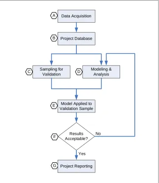
This section describes the strategy employed to develop a multiple linear regression model to predict the PE percentage for bridge projects. Figure 1 summarizes the strategy graphically. The tasks labeled A, B, and C are complete and are reported on herein. The initial performance of Task D is also complete, but model revisions are anticipated after the validation results of Task E have been completed.

Data Sources Utilized for Data Acquisition (Figure 1, Task A)

Ten data sources were investigated and project data were successfully extracted from eight of the ten sources. The sources consisted of the following:

1. NCDOT Online Bid Tabulations & Annual Bid Averages Summary

2. NCDOT Pre-2002 Project Management Data System (obsolete mainframe system) 3. NCDOT Post-2002 Project Management Data System (SAP based)

4. NCDOT 12-Month Projected Letting List

5. NCDOT National Bridge Inventory System Data (NBIS) 6. NCDOT State Transportation Improvement Plan (STIP) 7. North Carolina State Publications Clearinghouse

(5)

9. NCDOT Online Construction Plans (not used for extraction)

10.NCDOT Board of Transportation Agendas and Meeting Minutes (not used for extraction) Project data were not obtained from online construction plans (source 9) because plans were not available for all 505 bridge projects. Online plans became available starting with projects let in August 2004. Projects dating back to January 1999 were used in model building. Online Board of Transportation meeting agendas and minutes (source 10) were available in a PDF format. However, the PDF document format did not support efficient searching (utilizing multiple criteria) to extract specific project data.

Project data from the remaining eight sources were grouped by data function: classification, cost, date, design, dimensional, environmental, and geographical. Table 1 lists the 28 independent variables (grouped by category) identified for each bridge project.

Values for the 28 independent variables shown in Table 1 were acquired from the first eight sources mentioned above for 505 North Carolina bridge projects let for construction between January 1, 1999 and June 30, 2008.

Figure 1. Regression Modeling Flowchart

Data Acquisition

Project Database

Sampling for Validation

Modeling & Analysis

Model Applied to Validation Sample A

C

B

D

E

F

G Project Reporting Results Acceptable?

No

(6)

Table 1. Independent Variables (28) for Bridge Data Analysis

Category Independent Variable Variable Levels or Values

Project Construction Scope New Location, Replacement, Culvert

Number of Lanes on Bridge Numerical Count

Type of Service on Bridge Highway, Railroad, Pedestrian

Route Signing Prefix Interstate, US Hwy, State Hwy

Capacity Rating of Live Load Metric Tons

Road System Arterial, Collector, Local

Classification

Structure Type Bridge or Culvert

ROW Cost to STIP Estimated Construction Cost Cost Ratio

Roadway Percentage of Construction Cost Cost Ratio Cost

STIP Estimated Construction Cost Cost in Dollars ($)

Year of Letting Calendar Year

Year of Environmental Document Approval Calendar Year Date

PE Duration After Environmental Doc Days

Deck Structure Type Concrete, Steel, Aluminum, Wood

Design Live Load M9, M13.5, MS13.5, M18

Main Span Structure Type Concrete, Steel, Wood, Masonry

Design

Design Type Slab, Girder, Box Beam, Truss

Project Length Feet

Bypass Detour Length Kilometers

Number of Spans in Main Unit Numerical Count

Horizontal Clearance for Loads Meters

Length of Structure Meters

Dimensional

Water Depth Feet

NEPA Document Classification EIS, EA, CE, PCE, Min Criteria

Environmental

Planning Document Responsible Party NCDOT or PEF

NCDOT Division DIV 01 through DIV 14

Geographical Area of State Coast, Piedmont, Mountains

Geographical

Classification of Route Rural or Urban

Database Adjustments for the Preferred Response Variable (Figure 1, Task B)

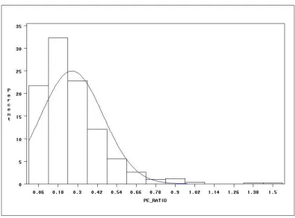
For the 505 bridge projects database, a ratio of PE costs to construction costs was desired as the response (dependent) variable. Using a cost ratio rather than actual cost values allows comparisons to be made among projects having differing construction costs. The ratio of actual PE cost to the estimated STIP construction cost was tabulated for all 505 projects. This ratio is referred to as the project’s PE Ratio.

(7)

distribution would have a center interval as the peak with decreasing intervals symmetrically located both left and right of the peak.

Figure 2. Distribution of Response Variable “PE Ratio”

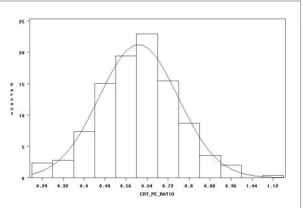
Power transformations were applied to the response variable, PE Ratio, to improve normality. The response variable was raised to an exponential power resulting in a transformed variable. Applying the Box-Cox statistical procedure to the nonnormal response distribution identified the optimal normalized distribution as the cube root of PE Ratio, (PE Ratio)1/3. Figure 3 shows the distribution for the transformed response variable, Cube Root of PE Ratio; the distribution is normal. Subsequent regression analyses use Cube Root of PE Ratio as the response (dependent) variable.

Normality of the response variable is sought to satisfy multiple linear regression assumptions. Those assumptions are that regression errors are independent, exhibit a constant variance, and be normally distributed. The requirement that error is normally distributed is interpreted to mean that the response variable is normally distributed at all values of the predictor variables. Thus, a normal distribution of the response variable is desired.

Sampling for Validation (Figure 1, Task C)

(8)

set. This set size is 15 percent of the bridge database. The remaining 430 bridge projects were used for model building.

A prediction for a within-sample project is statistically stronger than an out-of-sample project prediction. When using within-sample projects, the full range of values for independent variables have been included in model building. The same is not true with out-of-sample projects. Using past projects (a historically based model) to predict future project performance is considered an out-of-sample prediction. There is no way to know if a future project’s actual independent variable values will fall within the range of historical values used in model building. The intended use of the model is primarily for future project predictions. Out-of-sample validation projects were included to strengthen the validation process.

An additional out-of-sample validation set was created from 46 bridge projects not included in the original 505 bridge projects database. These 46 projects satisfy three criteria:

• Projects let for construction since July 1, 2008

• Projects included in NCDOT’s Structure Inventory and Assessment (NBIS) database

• Projects with identified PE costs

The within-sample projects (75) and out-of-sample projects (46) were combined to form a complete validation data set containing 121 bridge projects. Thus, the model was built using 430 bridge projects and will be validated using 121 projects.

(9)

Model Selection Techniques (Figure 1, Task D)

Simple linear regression (SLR) offers a mechanism to determine the linear relationship between one independent variable and the response (dependent) variable. However, SLR has only limited use because all of the other independent variables and the interrelationships between them are ignored. Multiple linear regression (MLR) overcomes the limitations of SLR. However, selecting the “best” model using MLR can be difficult if there are a large number of independent variables. Common model selection techniques involve forward, backward, and stepwise variable selection methods. To assist in model selection, the GLMSLECT procedure within SAS statistical software was utilized. In addition to forward, backward, and stepwise, GLMSELECT provides two additional variable selection methods: least angle regression (LAR) and least absolute shrinkage and selector operator (LASSO). The GLMSELECT procedure provides an efficient starting point for model selection. Model refinement can then follow using intuitive insights gained from data familiarity. [Cohen 2006]

FINDINGS

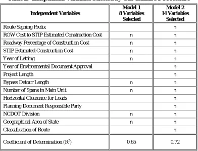
Using the GLMSELECT procedure with SAS statistical software, two candidate models containing eight and fourteen independent variables were selected. Table 2 identifies the independent variables in each model.

Table 2. Independent Variables Selected by GLMSELECT Procedure

Independent Variables

Model 1 8 Variables

Selected

Model 2 14 Variables

Selected

Route Signing Prefix n

ROW Cost to STIP Estimated Construction Cost n n

Roadway Percentage of Construction Cost n n

STIP Estimated Construction Cost n n

Year of Letting n n

Year of Environmental Document Approval n

Project Length n

Bypass Detour Length n n

Number of Spans in Main Unit n n

Horizontal Clearance for Loads n

Planning Document Responsible Party n

NCDOT Division n n

Geographical Area of State n n

Classification of Route n

Coefficient of Determination (R2) 0.65 0.72

(10)

CONCLUSIONS

Although the validation process has yet to be completed, the resulting R2 values obtained indicate that regression modeling has potential as a prediction tool for PE costs. By considering numerous individual project factors (expressed as independent variables) a more accurate prediction for project PE costs can be developed. Multiple linear regression modeling shows promise as a tool to support improvement in PE estimate preparation and cost budgeting. With more accurate PE costs, combined with ROW and construction costs, state transportation agencies can better allocate funding resources to capital projects.

CONTINUING WORK

The regression model described has yet to be validated as illustrated in Figure 1, Task E. Once validation is completed, using the 121 bridge projects comprising the validation set, the model can be finalized (Task F). The optimal model will maximize the coefficient of determination values, R2 and Adjusted R2, while minimizing prediction error expressed by mean square error (MSE). After finalization, a user-friendly interface could be developed to provide a software tool to readily determine PE costs. In the meantime, additional work should be done with the model. Key remaining questions are what are the fewest number of parameters that are needed to obtain a good R2 value, and thus, a good prediction and what is the optimum number of parameters?

Advanced statistical techniques such artificial neural networks and fuzzy logic can be used to overcome the assumptions that are necessary when using multiple linear regression, most notably that the predictors and response be linearly related. Other potential advantages include the ability to address complex interactions between predictors, and modeling the subjective nature of predictors when deterministic data are unavailable. We are continuing to study whether or not use of such alternate techniques yields an improved prediction model for PE costs of bridge projects.

ACKNOWLEDGEMENTS

The authors acknowledge the project support provided by the NCDOT Research and Development Unit. Key NCDOT units providing guidance include the Program Development Branch (Calvin Leggett and Majed Al-Ghandour), the Structure Inventory and Appraisal Unit (Cary Clemmons), and the Schedule Management Office (Kim So, Rose Simson, and Anna Twohig). Many additional NCDOT personnel have provided suggestions and insights. Their contributions continue to influence this research effort in a positive manner. The authors also thank the Southeastern Transportation Center whose early support was instrumental in transitioning this research topic into a funded project.

(11)

REFERENCES

Cohen, R. A. (2006). “Introducing the GLMSELECT PROCEDURE for Model Selection.” Proceedings of the Thirty-first Annual SAS Users Group International Conference, SAS Institute Inc., Cary, NC. Paper 207-31. <http://www2.sas.com/proceedings/sugi31/207-31.pdf>

Knight, K. and Fayek, A. R. (2002). “Use of Fuzzy Logic for Predicting Design Cost Overruns on Building Projects.” Journal of Construction Engineering and Management, American Society of Civil Engineers, Reston, VA. 128(6), 503-512.

Kyte, C. A., Perfater, M. A., Haynes, S., and Lee, H. W. (2004a). “Developing and Validating a Highway Construction Project Cost Estimation Tool.” Virginia Transportation Research Council, Report 05-R1, Charlottesville, VA. <http://vtrc.virginiadot.org/PUBDetails.aspx? Id=296398>

Kyte, C. A., Perfater, M. A., Haynes, S., and Lee, H. W. (2004b). “Developing and Validating a Tool to Estimate Highway Construction Project Costs.” Transportation Research Record,

Transportation Research Board of the National Academies, Washington, DC. (1885), 35-41. Lowe, D. J., Emsley, M. W., Harding, A. (2006). “Predicting Construction Cost using Multiple Regression Techniques.” Journal of Construction Engineering and Management, American Society of Civil Engineers, Reston, VA. 132(7), 750-758.

Odeck, J. (2003). “Cost Overruns in Road Construction – What are Their Sizes and Determinants?” Transport Policy, World Conference on Transport Research Society, Lyon, France. 11(2004), 43-53.

Sheiner, L. B. and Beal, S. L. (1981). “Some Suggestions for Measuring Predictive Performance.” Journal of Pharmacokinetics and Biopharmaceutics, Springer Healthcare Communications Ltd, New York, NY. 9(4), 503-512.

Turochy, R. E., Hoel, L. A., and Doty, R. S. (2001). “Highway Project Cost Estimating Methods used in the Planning Stage of Project Development.” Virginia Transportation Research Council, Technical Assistance Report 02-TAR3, Charlottesville, VA. <http://vtrc.virginiadot.org/ PUBDetails.aspx?Id=296547>

(12)

AUTHOR CONTACT INFORMATION

Donna A. Hollar Teaching Instructor East Carolina University

Department of Construction Management Rawl Building, Room 329

Greenville, NC 27858-4353 Phone 252-328-6968 Fax 252-328-1165 Email [email protected]

Ingrid Arocho PhD Student

North Carolina State University Department of Civil Engineering Campus Box 7908

Raleigh, NC 27695-7908 Fax 919-515-7908 Email [email protected]

Joseph Hummer Professor

Raleigh, NC 27695-7908 Phone 919-515-7733 Fax 919-515-7908 Email [email protected]

Min Liu

Assistant Professor