On vortex/wave interactions. Part 1. Non-symmetrical input and cross-flow in boundary layers

Journal of Fluid Mechanics

http://journals.cambridge.org/FLM

Additional services for Journal of Fluid Mechanics:

Email alerts: Click here Subscriptions: Click here Commercial reprints: Click here Terms of use : Click here

On vortex/wave interactions. Part 1. Non­symmetrical input 

and cross­flow in boundary layers

S. N. Brown and F. T. Smith

Journal of Fluid Mechanics / Volume 307 / January 1996, pp 101 ­ 133 DOI: 10.1017/S0022112096000067, Published online: 26 April 2006

Link to this article: http://journals.cambridge.org/abstract_S0022112096000067

How to cite this article:

S. N. Brown and F. T. Smith (1996). On vortex/wave interactions. Part 1. Non­symmetrical input and  cross­flow in boundary layers. Journal of Fluid Mechanics, 307, pp 101­133 doi:10.1017/

S0022112096000067

Request Permissions : Click here

J. Fluid Mech. (1996), vol. 307, pp. 101-133

Copyright 0 1996 Cambridge University Press

101

On vortex/wave interactions. Part

1.

Non-symmetrical input and cross-flow in

boundary layers

By S. N. BROWN A N D F. T. SMITH

Department of Mathematics, University College, Gower Street, London WClE 6BT, UK

(Received 5 September 1994 and in revised form 1 1 August 1995)

The paper studies certain effects of non-symmetry on vortex/wave interactions, for inviscid inflexional waves interacting nonlinearly with the vortex component of the mean flow in boundary-layer transition at large Reynolds number. Two types of non- symmetry are investigated, namely for unequal input wave amplitudes and for small cross-flows. These lead to coupled integro-differential equations for spatial de- velopment of the wave amplitudes, which are examined in an essentially equivalent differential form for various degrees of the non-symmetry present. Each type of non- symmetry can have a significant influence on the nonlinear interaction properties. Special emphasis is given to bounded solutions, and numerous interesting new flow responses are found analytically and computationally. The theory provides a basis for tackling enhanced non-symmetry in the input or stronger cross-flows.

1. Introduction

Vortex/wave interactions in boundary layers, channel flows and related motions have attracted considerable attention recently with regard to transitions from laminar flow. These nonlinear interactions arise in various forms, principally with viscous- inviscid Tollmien-Schlichting waves or with inviscid inflexional Rayleigh waves as in Hall & Smith (1988, 1989, 1990, 1991), Walton & Smith (1992), Blennerhassett &

Smith (1992), Stewart & Smith (1992), Smith & Bowles (1992), Walton, Bowles &

Smith (1994), Benney & Chow (1989), Goldstein & Choi (1989), Brown et al. (1993), Smith, Brown & Brown (1993, referred to herein as SBB), Wu (1993a), Wu, Lee &

Cowley (1993) and Khokhlov (1994) in different flow regimes. They all have the common feature, however, that at high Reynolds numbers small-amplitude three- dimensional waves are coupled nonlinearly with the mean flow via its unknown longitudinal vortex component. The remarkable smallness of the waves involved, especially in SBB, is in fact one reason on both practical and theoretical grounds for the attention devoted above to vortex/wave interactions, in comparison with the somewhat higher amplitudes connected with nonlinear triple-deck interactions and the still higher amplitudes in Euler-scale interactions. More detailed comparisons are made by Hall & Smith (1991), Walton & Smith (1992), SBB and Timoshin & Smith (1995). A second reason for the theoretical focus on vortex/wave interactions surrounds the qualitative and quantitative links with experiments on transition described by Hall &

102 S. N . Brown and F. T. Smith

Nishioka, Asai & Iida (1979) and computationally by Wray & Hussaini (1984), Spalart

& Yang (1987), Kleiser & Zang (1991), Sandham & Kleiser (1992), Rempfer & Fasel (1994) (and many references therein) for example. Third, and perhaps from a narrower perspective, vortex/wave interactions yield a wide range of interesting new analytical/ computational problems in transitional fluid dynamics.

The concern of this paper is with the effect of non-symmetry on vortex/wave interactions in the presence of inflexional disturbances, as opposed to the symmetric configurations studied by SBB and in the papers referenced in the preceding paragraph. The non-symmetry discussed in the present paper, Part 1, is due either to non- symmetrical input waves, or to cross-flow in the incident boundary layer. (Part 2, Brown & Smith 1996, is concerned with the effect of swirl in a jet flow) or both. The effects produced can be substantial in certain parameter regimes. Even quite small cross-flow or swirl for instance is found to have an important influence on the interactions, which is a significant practical point since in reality most incident boundary layers are likely to be three-dimensional to a greater or lesser extent, especially on swept wings, near wing-body junctions or in atmospheric boundary layers (see, for example, Reed & Saric 1989; Kohama, Saric & Noos 1991); similar considerations apply to swirling jets and similar flows with their possibility of inducing vortex breakdown. Along with that there is also the need to discover more about the impact of small non-symmetrical disturbances and cross-flow or swirl as well as input frequencies, wavenumbers and disturbance amplitudes, in devices intended to promote or delay transition efficiently.

The theoretical approach used is based on that developed in SBB. A predominantly two-dimensional inflexional boundary layer flowing in the streamwise direction x, but with a small amount of cross-flow in the spanwise direction z, approaches the neutral station x = 0 at which small inviscid three-dimensional Rayleigh waves are initiated and interact nonlinearly with the induced three-dimensional mean flow. The waves are of relatively short length and time scales whereas the induced vortex is relatively long and quasi-steady. The small cross-flow and the input non-symmetry are such as to affect the local nonlinear interaction substantially. In due course a study of much stronger cross-flows would be desirable, bringing in full cross-flow modes nonlinearly, cf. Stuart (1963), Hall (1986), Stewart & Smith (1987), Bassom & Gajjar (1988), Gajjar (1995) and the strong cross-flows accommodated in Davis & Smith (1994) for longitudinal vortex interaction with viscous-inviscid waves, but the above approach seems to provide a helpful starting point. The local cross-flow structure then is multi- zoned in the direction normal to the solid surface or wall y = 0, as in SBB, with a thin critical layer and two slightly less thin buffer layers lying in the middle of the boundary- layer core of the motion. The resulting nonlinear vortex/wave interaction involves interplay between properties in all the above zones.

On vortex/wave interactions. Part 1 103 general periodic forms are derived; in 99 forward-marching results are described for moderate values of L, N , where the parameter L is the ratio of the real and imaginary parts of a coefficient in the amplitude equations. Further comments are provided in

0

10.

2. The structure of the flow

The physical background of the problem is exactly as in SBB. The basic equations are the incompressible Navier-Stokes equations in non-dimensional form. With a representative length L* and representative speed U * , we write the starred dimensional Cartesian coordinates (x*, y*, z*), velocity components (u*, v*,

w*),

pressure/density ratio p*/p* and time t* as

(x*, y*, z*) = L*(x, y , z), (u*, v*,

w*)

= U*(u,

v,

w),l

p*/p* = u*zp, t* = U*t/L*.

J

(2.1)

The Reynolds number R defined as

R = U*L*/v*, (2.2) where v* is the kinematic viscosity of the fluid, will be taken as large throughout.

As in both Brown et al. (1993) and SBB and the earlier paper of Hall & Smith (1991), the boundary layer of width O(R-9 develops on a streamwise length scale O(R-b)

where 6

>

max(0, b). The transverse development is on a scale O(R-7 and it is convenient to write

x = R-bX, y = R-$i, z = R-". (2.3) A two-dimensional boundary layer, for example a classical boundary layer for which b = 0 and

S

=

+

in (2.3) or an interactive boundary layer with b =

&

S

=

i,

is assumed to attain the station

x

= 0 with a velocity profile U,,(p) that has a point of inflexion at

p

=

a,.

This neutrally stable profile initiates the three-dimensional nonlinear development of the flow, a development termed vortex/Rayleigh-wave interaction. Downstream of

x

= 0 a critical layer is present, consisting of a (unknown a priori) surface

p

=Ax,

3

of which the leading edge is the straight line X = 0,

p

= 8,. Both in SBB and the present work we are concerned with the immediate neighbourhood of the station

x

= 0 and we define

x

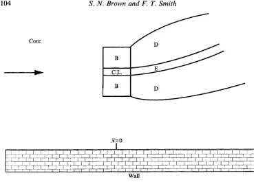
= e3x1, where e = R-(S-b)/6, (2.4) so that x , = 0(1) in what follows. The asymptotic structure of the flow is exactly as in SBB and is illustrated in figure 1. The core flows have

p

= 0(1), while in the buffer layers and critical layer the appropriate scalings are

p-AX,

3

= €3/2

r,,

F - f l X , F) = Y (2.5)

respectively. There is also a passive viscous layer on the wall of thickness O(s3), the effect of which is easily incorporated.

The final important scalings define fast variables in time and in the streamwise direction by

with the notation E reserved for the exponential

T = R3'-'-lt, a, X = R6-b a($ dX (2.6)

(2.7) In (2.6) and (2.7),

D

is a prescribed real frequency and the real wavenumber a($ is to be determined as part of the solution. The component of the solution that has a factor

s

104 S. N . Brown and F. T. Smith

Core

____)

x=

0 I

Wall

FIGURE 1. Sketch of the short-scale vortex/wave interaction region. The buffer layers B and the critical layer C.L. are in the region X = O(2); regions D and E represent their continuation into

x

= O(1).

E (or products of its powers and inverses that do not make a zero exponent) is known as the wave, while the E-independent component is termed the vortex. In SBB the leading-order wave pressure, i.e. that of the input wave, was taken to be of the form

r(xl)

P&y)

E C O ~ , ~ ~ Z + C . C . , (2.8) where Po($ is an eigensolution of Rayleigh’s equation and /lo is a prescribed constant wavenumber in the ,%-direction. The result of the investigation was an integro- differential equation (of cubic nonlinearity) for the amplitude r(xl). In the present study we replace (2.8) by

gpO(y) E{r+(xl) eijoz+ r-(xl) e-iPoz}

+

C.C.

If we regard (2.8) as typifying a pair of waves at angles +/3,/a0 to the mainstream direction with equal amplitude r(xl), then correspondingly the pair of waves in (2.9) have the possibility of unequal amplitudes r+(xl) and r-(xl).

In the following section we describe the amendments that must be made to the integro-differential equation of SBB, firstly due to the input wave (2.9) and secondly due to a small z-independent transverse cross-flow component to the oncoming boundary layer.

On vortexlwave interactions. Part 1 105

O(e3), contribution in the z-direction to the oncoming two-dimensional boundary layer. The reason for the choice of order of magnitude of this contribution is that it affects the core flow at the same level in the series expansion as does the non-parallelism of the basic flow. The corresponding effect on the buffer and critical layer is discussed after (3.13).

The equation obtained and analysed in SBB is

where the constants which comprise the coefficients are as follows:

C, = U,(a,), b, = Uh(a,), b, = U;(Z,), y: =

a:+P:.

(3

4

Also, G i - G;, G i - G; are integrals of the basic flow, and Q; is the contribution from the wall layer. The definitions are

and Q; = - ?:

P,(O)

(- ia, cO)-'I2. (3.4)

a(x) = a,

+

e3a2 X ,

+

0(e3) ₍₃ * 5) and x , U, is the O(e3) correction to the mainstream in the core region.

In (3.1) the linear terms would arise if there were no vortex-wave interaction. The nonlinear term results from the discontinuity across the critical layer in the transverse shear stress in the buffer region, and its coefficient ( A say) is obtained by solving the equations that are valid in the neighbourhood of the critical layer. In SBB it was necessary to select the coefficient of cos

Po

z in

In (3.3a), a2 is the coefficient of x , in the expansion of a(x) in (2.6) as

where

and

T,(x,,g =

r1

J,(s,ads J -00

(3.7)

Here p"o(x1,23 = cos P o

z

(3-9)

and J,(s,

mentioned above.

we must now select the coefficients of e+igor in (3.6) with

is the jump across the critical layer in the transverse shear stress that was

In the new study, in which (2.9) replaces (2.Q to obtain the two equations for r+(xl) -

(3.10)

106 S. N , Brown and F. T. Smith

The linear terms in equation (3.1) have r(xl) replaced by r+(xl) respectively while the nonlinear terms become, again respectively for the ekipoz contributions,

(3.11)

where the asterisk denotes a complex conjugate.

We now assume that the body is yawed to the oncoming boundary layer so that there is a ,%direction component, e3W0(7), for the mainstream velocity. The effect of this modification on the flow in the core is to replace a. x, U, by a, x, U,

k

Po

W,

for the two equations respectively, so that the right-hand side of (3.1) is augmented by a term

where (cf. (3.3)) (3.12)

(3.13)

In the buffer regions and the critical layer, the only property of Wo that is relevant is its value at the critical layer, W(a0) = go say. In both regions the operator

c0a,.

is replaced by c, 3%’ +go

az

which is equivalent to co dZl f iPo go when applied to the terms displayed in (3.10). The first term in (3.1) is a phase-jump contribution to the buffer layer and we must replace co r’,(x,) here by co r’,(xl) f @,go r+(xl). The integral in the nonlinear term results from the inversion of a Fourier transform with respect to x1 obtained as a solution of the buffer-layer equation for the leading contribution to the vortex, namely

(c,

a,.,

+go

a 3

wo = WOY,Y,* (3.14a) Equation (3.14a) is to be solved, as in SBB where go = 0, with wo + 0 as x, + - co and as

q,

the buffer-layer normal coordinate, tends to infinity. Also the jump (3.8) forced by the critical layer leads to a discontinuity Jo(xl,$ in

waul

across = 0. Since it follows from (3.8) that wo is a linear combination of terms in exp ( f 2iP0

3,

(3.14a) may easily be solved and (3.11) is now replaced by

(3.14 b)

as the nonlinear contribution.

Equation (3.14a) may be recognized as equation (3.7) of Part 2 with ro 0 identified with rand 6, withg,. Indeed the analysis of the buffer and critical layers, presented here as a straightforward extension of SBB, may be deduced from the more intricate calculation of Part 2 in the limit ro+co with n/r, fixed.

Finally we make the transformations

(3.15)

so that the appropriate analogues of (3.1) are

Ct’,(x,)+At,(x,) t+(s) t*,(s)ds+(Bxl+F+)t+(xl) - - = 0, (3.16)

which may be compared with (6.1) of SBB. The constants A , B, C have the same values as in SBB where A was real and C complex. In SBB the value of B was taken to be real as there the discussion was restricted to profiles such that the solution in the region

On vortexlwave interactions. Part 1 107 under consideration had the possibility of a match with the initiation of the Hall-Smith vortex/wave interaction as analysed in BBST. If this restriction is removed and a more general class of downstream development is examined, as it will be here and also was in SBB, then the requirement of a downstream limit with a regular critical layer for a match with the Hall-Smith solution is no longer necessary. The result is that Bin (3.16) can be complex. A complex B makes no difference to the analysis of the solutions of the amplitude equation that were carried out in SBB. Also in (3.16)

(3.17) Here

D,

G are real

(D

by a change of origin of x,). In addition A , B,

C,

D

are functions of /3: as are G i , G', and hence it is only the real parts of F+ - that differ in the constants in the two equations (3.16).

Integro-differential equations resembling (3.16) arise in discussions of the nonlinear evolution of instability modes in laminar boundary layers and shear flows in many of the references cited early in the introduction. The motivation behind the derivation of the corresponding equation of SBB, to which (3.16) reduces in the equal-amplitude case t, = t- with

F+

=

E ,

was to analyse the development of the amplitude t+(x,) on a streamwise length scale that permitted a match downstream with the small-x solution of the Hall-Smith vortex/wave-interaction equations which hold when x of (2.3) is O( 1). In the Hall-Smith structure it is anticipated that the coupled reaction between the oblique Rayleigh waves and the developing mean-flow results in an evolving regular viscous critical layer of equilibrium type, and that the self-sustaining interaction will persist to large distances downstream. In SBB, of which the present study is a generalization to unequal amplitudes of the input waves and to cross-flow, the shorter lengthscale x = O(e3), i.e. x1 = O( l), is considered, and critical-layer interaction, again of a viscous equilibrium type, between two oblique waves of amplitude O(e7) forces a spanwise-dependent (vortex) contribution of smaller order O(e8). In addition to the Hall-Smith limit the equation of SBB generates three other possible solution paths of interest in their own right.

By contrast the integro-differential equation of Wu et al. (1993) involves multiple integrations, a more complicated kernel, but no non-parallel term. These authors study oblique input waves of equal amplitude in an analogous problem of an unsteady shear layer but work on a shorter length scale (there a time scale) equivalent to x = O(e4)

here. In their situation the critical layer is of non-equilibrium type, since the streamwise gradients are larger, the buffer layer is absorbed into the critical layer, and the spanwise-dependent mean flow is induced at the same order, O(e6), as the input wave. The inviscid limit of these authors' amplitude equation reduces to that of Goldstein &

Choi (1989), and in a discussion of the relation between their approach and the Hall-Smith vortex/wave interaction theory, they demonstrate that in a certain viscous limit it can be reconciled with that of SBB without the non-parallel term. Further explanation of the various length (time) scales involved is given by Wu & Cowley (1995). The same shorter x-scale and non-equilibrium critical layer is involved in the resonant-triad studies of, for example, Wu (1995).

Most studies to date have been confined to symmetrical situations, i.e. the oblique waves make equal angles with the direction of the undisturbed mainstream and are of equal amplitude. An example without these restrictions is that of Wu (19933) which, although an examination of the development of a triad of Tollmien-Schlichting waves rather than Rayleigh waves as considered here, leads to a pair of equations of the form (3.16) together with one for the two-dimensional wave. His equations effectively have C purely imaginary, and his numerical solutions show that interaction with the two-

108 S. N . Brown and I;. T . Smith

dimensional wave can result in two oblique waves of unequal input amplitude evolving to an equal-amplitude state. Equations (3.16) have complex constants and a non- parallel term and hence a very rich solution space. For any non-zero cross-flow, i.e. non-zero G in (3.17), equal amplitudes will not be a possibility here.

The following sections are devoted to a study of equations (3.16) with emphasis on parameter values that will result in solutions that are expected to persist at large distances downstream, and on the effects of the cross-flow.

4. The governing ordinary differential equations

In this section we rewrite equations (3.16) as differential equations for the modulus and phase oft, by eliminating the integrals and separating the resultant equations into their real and imaginary parts. We define successively

and for the constants appearing in (3.16) we let

C

= h

+

ip, B = a

+

i7 and define L, M ,

N by

L2 = h2/p2, M = (ha+p7)/(h2 +p2), N = Gh/(h2 +p2). (4.3)

The equations for the phases 8, - are then

4ApR+

e+

= h2T'-p2S'+2(Dp+ Gh) S+2x1(hnT-p7S), 4hpR-

6"

= - h 2 T ' - ~ 2 S ' + 2 ( D p - G h ) S - 2 x 1 ( h ~ T + p ~ S ) .

The change of origin

(hV +p7) X , - Dp = (ha +p7) X _(4.5) enables the constant D to be eliminated from the modulus equations. With a final transformation

these equations are S(X) = ~ , ( x ) e - ~ ~ ' ,

~(x)

= ~ , ( x ) e - ~ ~ * (4.6)

- - ~ h e - ~ ~ ~ ( s f - T ; ) ~ / ( A ~ +p2), ( 4 . 7 ~ ) ( S

;

- T ;) Sy = S,( S;Z

+

L2 Ti2)

+

4NS,{L2S, T i

+

q

S ;

+

N( 1

+

L2) Sf}

(Sf- Tf) T i = - T,(Ti2 +L-'S?)+ 2N{(1 -LP2) Tf Si

- ( 1 + C 2 ) Sf Si -2S1

q

T ; -2N(1+ L-') Sf

T }

(4.7b)

with the parameters L, M , N, Ah/(h2 + p 2 ) remaining.

In SBB, all the solutions of equations (4.7) were found in the special case of N = 0 with also = 0. This is the completely symmetric situation with zero cross-flow, and two waves of equal amplitude equally inclined to the mainstream direction. With N =

T = 0 the behaviour of the solutions depended only on the signs of M and Ah. With M

>

0 and Ah

<

0 there were four possibilities. The first, in which the solution terminates at a saddle point in the phase plane as

x

+co with a non-zero constant limit for S (not for S,), is that which matches with the initiation solution of the Hall-Smith

(1991) wave/vortex equations as discussed in Brown et al. (1993). This solution is unique. The other solutions for S either decay both as x + k c o , exist between two algebraic singularities, or decay at one end and terminate at a finite value of

x

at the other. With A4

>

0, but Ah

>

0, only the decaying solutions are possible. If M

<

0 and

On vortex/wave interactions. Part 1 109

were the subject of extensive discussion in SBB as it was believed that the resulting self- sustaining waves on a flow which is nevertheless changing structure would be applicable to the early phases of laminar-turbulent transition.

Equations (4.7) may be regarded as replacing equations (3.16). In addition, however, because of the differentiation of (3.16) involved above, there are constraints on the appropriate starting conditions for (4.7); these correspond to requiring Ct; = - (Bx,

+

F+) t , at the start of the interaction where nonlinear effects are negligible. It may be shown that this reduces to

as a starting requirement. Further reference to (4.8) is made in the following section. In the following section we submit the governing equations (4.7) to a further simplification with a view to computing and analysing solutions of a periodic or self- perpetuating form.

Si+2NT, = 0, T ; + 2 N S l = 0 (4.8)

5. A limiting form of the governing equations

The solutions of equations (4.7) discussed in SBB that persisted on a large stream- wise scale were (with N = T = 0) the periodic solutions for S. These, at large values of the typical amplitude, exhibited long regions of predominantly vortex flow interrupted by rapid vortex/wave interactions which continually moderated the vortex flow. The first of these is a non-parallel phenomenon while the second is a short-scale quasi- parallel readjustment. For this interpretation of the solution it was necessary first to consider x p 1, and then to have M

<

0 and Ah

>

0 so that the periodicity conditions were satisfied. We now discuss equations (4.7) under similar conditions. We assume that x remains within an O(1) (or less) distance of X , where X ,

>>

1, change the origin to X,, and replace the factor

cMX2

multiplying the quartic terms in (4.7) by e-MX:

.

Because of the scaling properties of (4.7) it is then sufficient to replace

Ah e-MXi/(h2 +p2) by f 1 and, by analogy with SBB since this produced the solutions of greatest interest, we choose the positive sign. Although this argument can be carried through regardless of the sign of M , the resulting solutions are expected to be of most significance when M < 0 because if M > 0 it is likely, (see (4.6)), that S, T will be exponentially small. Negative M was required for the periodic solutions of SBB.

With Ah e-Mz2/(h2 +p2) replaced by unity, as explained above, (4.7) can, by addition and subtraction, be put in the form

M W

-

ABA“ = @2(A”’ -

2

) 2

+

(A”’

+

2 ) 2 ] [( 1 - L-2)

A”+

(1

+

L-2)

B”]

- A”zB”2 +;N{(A”’-B)(L2(A”+B”)2-A”2+B”2)

+

(A”’

+

2)

( 2 -

B2

- 22B”- L-2(2

+

@))}

+;N2(A”+ip{(I +L2)(A”+B”)-(1 +L-2)(2-B”)}, (5.1 a)

--

-

A B B =

Q[L2(A”’-B”’)2+(A”I+B”’)2][(1+L-2)A”+(1-L-2)B”]-J2B”2

+;N{(A”I--) (L2(A”+B”)2+A”2-B”2)

+;N2(A”+B”)j2{(1 +L2)(A”+B”)+(1 +L-2)(A”-ii)}, (5.1 b)

+

(A”’

+

2)

(A”” -

9

+

2 2 8

+

L-2(22

+

P))}

containing the two parameters L, N, where

A”=

s,.tT,,

B”=

s,-T,.

(5.2)

110 S. N . Brown and F. T. Smith

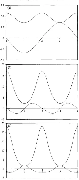
(5.2) is associated with extreme conditions such as large typical amplitudes, input far upstream, large-amplitude input, and/or extreme values of A , M in (4.7), these conditions are in fact very interesting physically, particularly the applications to increased amplitudes. This point is made in SBB. As there, and as indicated in the previous paragraph, we would expect a non-parallel-flow effect to re-enter, from (4.7), even further downstream probably on the longer O(X,,) scale in x. Finally, the starting requirements (4.8) are not expected to impose any great restrictions on the current solution. Some of the solutions of (5.1) that we shall obtain satisfy them automatically in the region under consideration (see for example figure 3 (a, c) for which N = 0 and Sl, and T i repeatedly have common zeros). Those solutions that do not satisfy (4.8) in the present region of interest are assumed to correspond to wave profiles that have evolved in an upstream region where the requirements were satisfied.

Although equations (5.1) appear complicated it is possible to gain from them some feeling, by inspection, of the effect of the cross-flow parameter N . With N = 0, there is, for all L, a non-trivial solution with

A"

=

B

and non-constant. This is the solution of SBB with = 0. When cross-flow is present Land

B"

are not interchangeable unless the sign of N , or alternatively that of x, is also changed. If we recall that

x,

B"

represent amplitudes of imposed waves that are equally inclined to the x-axis, whereas the presence of the cross-flow implies a bias towards the direction of one or other of these waves, then the skew-symmetry is not unexpected. We note here, and it will be of interest in $9 below, the existence of the simple symmetric solution

A"

=

B"

= 4( 1

+

L2) N 2 .

In the following section we demonstrate analytically the existence of periodic solutions of (5.1) by asymptotic methods in which the asymptotically small parameter chose, B say, is a measure of the distance between the functions

A"

and

B".

It will, in addition, for the consistency of the analysis, be necessary to assume that N = O(3. The resulting period is asymptotically large.

6. Solutions for small cross-flow with amplitudes

A"

and equal

(5.1) have the solution

approximately

When A"and Bare taken to be equal and the cross-flow N set equal to zero, equations

% - a'lZ

A = B = asech2--((x-b),

d2

where a, b are arbitrary constants. This solution can, by suitable interpretation of the constants a, b, be recognized as that obtained in $7 of SBB when the periodic solutions of large amplitude were examined for x

+

1. It corresponds to a region of rapid vortex/wave interaction and is followed in that study by a long region of non-parallel predominantly vortex flow with negligible wave action. The cycle is then repeated because in the situation considered there (which has

3

= N = 0 in (4.7)) all solutions of (5.1) with Ah

>

0 are periodic functions of x. Our aim in this section is to show that the symmetric solution (6.1) can be used to construct non-symmetric solutions of (5.1) that are periodic functions of

x.

We shall find that there are also solutions of (5.1) that are not periodic functions.

The structure of the solutions of (5.1) that have

A"

z

B

is as follows. There are humps in which the sech2 solution of (6.1) is appropriate separated by troughs in which

A"

and

On vortexlwave interactions. Part 1 111 any constant a, so for simplicity we shall take a = 1 in (6.1) so that the maximum height in a hump is unity. It emerges that the matching requires the same value of a for each hump.

(a) The solutions in the humps

We let the successive humps have their maxima at x = 0, s,, s,,

...,

with, for the nth (6.2a) hump

&,) - B(s,) = 7,

F,

(6.2b)

where

F

acts as a book-keeping parameter measuring the distance between Land

B.

We assume 0 <

F

4 1. At present y n and 6, are at our disposal.

&,)

+

B ( S , ) = 2, A”’(s,)

+

B’(s,) = 0,

&s,) - B’(s,) = 6,

F,

The solution in the nth hump is thus

(6.3) 1

A”(x)

+

j(x)

= 2 sech2 __ (x - s,)

d 2 from (6.1) with a = 1, and from (5.1) on linearization

where X(x) - B(x) = FC(x),

-

2 1

-

1 1

C”(x)+-tanh2--(x-ss,) _{L d 2} C(x) = fisech2--(x-s,) _{d 2} tanh-(x-s,) _{d 2} (6.5)

N = 2-5/2 aV/(i

+

r2).

C(s,) =

Yn,

Cys,)

= 6, (6.7)

(6.6) if we set

The boundary conditions on (6.5) are that

to satisfy (6.2b). The solution of (6.5) may be written down by variation of parameters in terms of the solutions of the homogeneous equation. We denote these by $o(x), $,(x) where $o(s,) = 1, $;(s,) = 0, and $,(s,) = 0, $;(s,) = 1. To match with the solutions in the troughs we shall require the asymptotic forms of $o(x), $,(x) when Ix-s,I 9 1, which are

where yo, y,, q, r are constants depending on the value of L and are easily found numerically. It is not difficult to ascertain their asymptotic forms when L 9 1 and

L

<

1 and this is undertaken in the Appendix.

The solution of (6.5) that satisfies (6.7) is

z‘<x> = -$,(XI

Ln

H$, dx,

+

$,(XI

[

H$o dx, + 7% $,(4

+

6, $,(XI, (6.9)

where we have written H for the right-hand side of (6.5). It follows from (6.8) that for

Sn

x-s,

+

1,

(,’,

y,) (6.10)

-

rsinz

3-

C(x) z (7, -Il) q

but for x-s, 4 - 1,

-

C(x)

w

-(6,+Io)rsinz( L - z - y l ) . (6.11)

Here

112 S. N . Brown and F. T. Smith

and the facts that r$o is an even function of x -s, whereas r$l, Hare odd, have been used. The expressions (6. lo), (6.11) will be required for the match to the solutions in the troughs on each side of the hump centred on x = s,.

(b) The solution in the troughs

To leading order the solution in the troughs is obtained by ignoring the cross-flow terms proportional to N in (5.1) and the nonlinear terms

A”zB“z

on the grounds that they are smaller by a factor E“. The general solution of the resulting equations is, in the nth (6.13)

trough,

- -

A

+

B = p, cash (A,(x - t,)),

(6.14)

with four arbitrary constants An, p,, t,, h,. We now match the solutions (6.13), (6.14) to those in the hump, with suffix n say, behind this nth trough, and to those in the hump in front of it with suffix (n+ 1).

Matching

A”+B”

of (6.13) as x - & + - a with the solution (6.3) as x-s,+co first shows that A, = 2/2 and then gives a relation between p,, the minimum value of

A”+

B”

in the nth trough, and the difference between the x-coordinates of this minimum and the top of the previous hump. A similar relation is obtained by matching with (6.3), with n

+

1 replacing n, as x- t,+co and X-S,+~ -+ -

co,

s,+~ now being the position of the top of the succeeding hump. The two relations are

pu,/16 = exp[-2/2(t,-s,)l = ex~[-2/2(sn+,-tt,)l- (6.15) From (6.15) we first deduce that the trough is symmetrically between the two humps, and that the distance between the lowest point of the trough and the highest point of the hump is large, since (6.13) was derived on the assumption that p, =

O(9.

Further relations are found by the match of

A”-

B”.

As the nth hume is exited on the right, i.e. as x-ss,+0o, it follows that the asymptotic form of (A”-B)/E is exactly as given by the expression for c(x) in (6.10). However, as the (n

+

1)th hump is exited on the left, i.e. as x - s, --f - 00, the asymptotic form of

(2-

&)/B is given by the expression

in (6.1 1) with (n+ 1) for n. Both these asymptotic forms must match with

A”-B”

in (6.14). The match of the amplitudes leads to

(7% - 11)2q2

+

(6,

+

1olZr2

+

2(Y, - 11) (6,

+

10) qr cos 8

(6.16) Because of the simple sinusoidal form of

A”-B”

in the trough (see (6.14)) the phases of the asymptotic forms as the humps are exited must also be identical. The result of the (6.17) where

r:,

r;+,

are defined by

On vortexlwave interactions. Part

I

113 The interpretation of (6.15t(6.18) is as follows. If the conditions (6.2) are given at the hump x = s,, i.e. Eyn, E6, are given, then the position of the next hump,

x

= s,+~ and the corresponding values Y,+~, 6,+, may be obtained in terms of them. First, note that, since p, is known in terms of yn,, 6, from (6.16), (6.15) leads to

s,+1 -s, = d 2 log (16/p,). (6.19)

If we then write (6.17) as an equation for

Ti,,,

in terms of

Ti

which is known from (6.18a), and successively calculate sin

Ti+,,

cos

Ti,,,

equation (6.18b) may be solved as a pair of linear equations for Y,+~,

S,,,.

The procedure may be repeated from hump to hump. In the following section we examine solutions of this system of recurrence relations, showing that it has both periodic and non-periodic solutions. Subsequently we use the periodic solutions to construct periodic solutions of the system (5.1) of differential equations.

To complete the solution in the trough we require the constant h, in (6.14). Since the sinusoidal form of

A"-

B"

persists from the nth to the (n

+

1)th hump right throush the nth trough it is only necessary to match the phase of

A"-B"

to that given by C(x) in (6.10) as X-S,+OO on leaving the nth hump. The result of the match is that

h, = -(t,-s,)-Ti. 1.12 (6.20)

L

Here tn-s, is given by (6.15) and the match with the succeeding hump follows automatically on use of (6.17).

7. The recurrence relations

The system (6.18) is simpler in appearance if we write Eqy, = y , Eqyn+, = $7L Er(6,

+

Z,)

= 6, EI(&,+~ +Io) =

s",

p, = p, EqZ, = I so that, upon solving (6.18 b) for $7, 6 as suggested at the end of the preceding section, we obtain

2 L

(y -Z) sin- ( y o +yl - s)

+

6 ( y o - y,), (7.1 a)

2 2

L L

(y - I ) sin- (2y0 - s)

+

6sin- ( y o + y l -s) ( y o -yl). (7.1 b)

Here s = l0g(l6/p) (7.2)

and, from (6.16),

(7.34 2

L

p2 = (y - I ) 2 + 6'

+

2(y - I ) GCOS - (yo - y J ,

2 L

= ($7

+

Z)Z

+

8-

2($7

+

I ) s"C0S - (yo -yl). (7.3 b)

Given ( 7 . 3 ~ ) then (7.3b) is not independent of (7.1).

It is now clear that, given y, 6 we may calculate p from (7.3a), s from (7.2) and then

114

0

-1

-2

12

8

4

0

-4

- 8

- 12

1.5

1

.o

0.5

0

-0.5

S. N . Brown and F. T. Smith

On vortex/wave interactions. Part 1 115

12

8

4

0

-4

8

4

0

-4

-8

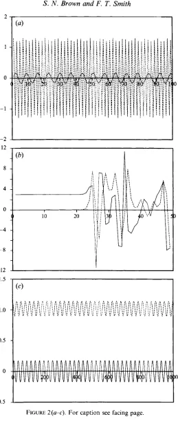
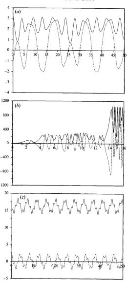
FIGURE 2. Solutions of the recurrence relations (7.1k(7.3) with initial conditions in the neighbourhood of those for a periodic solution (y continuous line, 8 dashed line): (a) stable with I = 0, L = 1 ; (b)

unstable with Z = 0, L = 1 ; (c) stable with I = 0.2728, L = 10; ( d ) unstable with Z = 0.5382, L = 10;

(e) unstable with Z = 2.9722, L = 1 .

(a) Periodic solutions

Although it is easy to compute successive

7,

$from (7.1)-(7.3) the system of recurrence relations is nonlinear, and as such may have unpredictable behaviour. We first examine the possibility of periodic solutions. It is not clear what the definition of periodicity should be but, initially at least, we shall consider periodic solutions for which the distance 4 2 s between successive humps is always the same. There is of course no reason why this distance itself should not be a periodic rather than a constant function. With ,u a constant it is not difficult to analyse the periodic solutions of (7.1)-(7.3).

At any stage the point

(7,8)

must lie on the ellipse (7.3b), and, when we update for the next stage it must also lie on (7.3 a). Thus the (up to four) points of intersection of these ellipses determine the periodic solutions with equally spaced humps. When I = 0 the

116 S. N . Brown and F. T. Smith

verified that (7.1)-(7.3) have the solution y = 0, 6 = p,

7

= 0,

s”=

p if (s-2yl)/L = pn for any integer p . Since p is asymptotically small, and hence s asymptotically large, for this theory to hold, strictlyp should be a large integer. In all there are four distinct possibilities, listed below, for periodic solutions with equal distances between humps. These are, where in each case p may be replaced by -p,

(i) y = 0, S = p,

7

= 0,

6

= (- l)pp with (s-2yl)/L =p77/2; (ii) y = p , S = O , ~ = ( - l ) p + l , u , s ” = O with (s-2y0)/L=p7r/2; (iii) y = 0, 6 = p,

7

= (- l)”+’p,

s”

= 0 with ( s - y O - y l ) / L = p77/2; (iv) y = p, S = 0,

7

= 0,

s”=

(- l)p,u with (s-yo-yl)/L =pn/2.

Case (i) with

-

p even and case (ii) with p odd are obviously immediately periodic (i.e. y = f , 8 = 8) with period d 2 s . If p is odd in case (i) and even in case (ii) then two applications are required before y, 6 return to their original values and the period is

23/2s. Cases (iii) and (iv) must be applied successively as a pair and the resulting period is 25’2s.

When I, which we recall is proportional to the cross-flow, is non-zero the original equations (5.1) and hence the recurrence relations (7.1) lose their upstream/ downstream symmetry. However, if purely periodic solutions are sought it is sufficient to restrict attention to positive I only because a change of sign of Nin (5.1) is equivalent to a change of sign of x. If I is sufficiently small the ellipses again intersect in four points, namely (0, S,), (0, S J ,

(7,

g),

(-

7,g)

where

-

.

(7.4)

I

(7-5)

L

-

L

r2

= ,u2-12tan2-((yo--y,), _L 6 = Zsec-(y,-y,) L and S,, S, are the roots of

2 L

= p2 - I 2 sin2 - ( y o - yJ.

Cases corresponding to (i)-(iv) of (7.4) are no longer all possible. One that does lead to a consistent eigenrelation for p is that corresponding to (i) with p even, i.e. y =

7

= 0, S =

s”

= CY,,~. The eigenrelation for this is found from (7.1) to be

1 2

p2 sin2 - (2y, - s) = I’ sin2 - ( y o - y,)

L L

with the corresponding

4 1

sin - (2yo - s)

sin - (2y, - s)

L

1 L S = I

(7.7)

(7.8)

Other combinations which might have been thought to have sufficient symmetry, for example y =

7

= 0 with 6 = S,,

s”=

S, or y =

7

=

-7

with

6

=

8=

s”

fail. The first clearly does not satisfy (7.3), while in the second the consequence of the lack of upstream/downstream symmetry is that although

7

may be followed by

-7

at the successive hump, it is not possible for the resulting

-7

to be followed by

7.

If 111

<

1, equation (7.7) reduces to

1 I 2

,(s-2yl) M m7c+-exp(2y1 16 +m7c)sin-(y0-y,) L

and (7.8) to

6 M f 16exp(-2y1-mn)

(7.9)

On vortex/wave interactions. Part 1 117 for integral m, both of which, as I+O, reduce to case (i) of (7.4) with p even. When L % 1, equation (7.7) requires IIL1 4 1 and ,u M IL/log(l6/IL) with, from (7.8), 6 M ,a.

To deduce these results, the asymptotic forms of yo, y1 in (AI) have been used. Although (7.7) has solutions for s, and consequently for y, when 111 % 1, in such a situation y = O(I) and although the recurrence relations have perfectly acceptable solutions in this regime these cannot be related to the solution of the original differential eguations for which it was assumed that 4 2 s is the distance between two maxima of A

+

B”

and thus essentially positive. Hence, from (7.2), it follows that no solution with y

>

16 is of direct interest; strictly the validity of the analysis is y -4 1. It is simple to examine the linear stability of the periodic solutions (iF(iv) in (7.4) with I = 0 and of the periodic solution given by (7.7), (7.8) for non-zero I. If in (7.lF(7.3) we write

y = y0+e1, 6 = 6 , + E 2 , y = yo+6y, s = so+6s, (7.11) where el, e2, Sy, 6s are small perturbations then, by linearization from (7.2), (7.3a), (7.1) successively we obtain

6s = - ~ y / y o , yo6y = ( 3 / 0 - ~ ) ~ , + ~ 0 ~ 2 + ( ( y , - I ) s 2 + 6 0 ~ 1 ) C O S ( Y , -

71,

(7.12a, b) Elsin(Y,-

Y,)

= elsin(&+ Y,)+e2sin2Y,

2 8,u

LPO

+--((yo - I ) cos

(Y,

+

Y,)

+

6, cos 2

Y,)),

(7.13 a)

E2sin(Y,-

Y,)

= elsin2Y,+e2sin(Y,+

Y,)

+--((yo 2 SP - I ) cos 2

Y,

+

6, cos

(Y,

+

Y,)).

(7.13 b) LPO

- *

Here jj = jjo

+

El, 6 = 6,

+

E2,

Y,

= (2y, -so)/&

Y,

= (2y1 -so)/L and we must substitute for S,u/,uo from (7.12b).

Equations (7.13) are linear recurrence relations with constant coefficients which may be solved exactly. If we write them as

(7.14)

u,+~ = au,

+

bv,, v,+~ = cu,

+

dv, then the condition for stability is that (hl

<

1 where h satisfies

h2-(a+d)h+ad-be = 0. (7.15)

It may be shown that each of cases (i)-(iv) of (7.4) leads to ad-bc = 1 so that if the roots are real then one has modulus greater than unity. If the roots are complex they both have modulus unity, and the perturbation, if initially of sufficiently small amplitude, will oscillate about zero. In cases (iii) and (iv) the roots of (7.15) are real for all yo, yl, so the situations are unstable. In case (i) the roots are complex if

cos(Y,- Y,)(cos(Y,- Y,)+Lsin(Y,- Yl))

<

0, (7.16) while in case (ii) the condition is

118 S. N . Brown and F, T. Smith

with even larger initial perturbations. However, an example of case (ii), again with

p = 1, is unstable owing to rounding error only; the instability is marked as can be seen in figure 2(b).

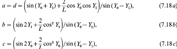
The values of a, b, c, din (7.14) for the periodic situation described by (7.7), (7.8) for non-zero I m a y be shown to be

2 L

sin(&+ Y,)+-cos &cos

Y,

(7.18 a)

(7.18 b)

(7.1 8 c)

Again ad-bc = 1 and the condition for the quadratic for h to have complex roots is now

(7.19)

1 1

L L

sin &sin Y,+-sin(&+ Y,)+,cos &cos

Y,

which reduces to (7.16), as it should, when so is given by case (i) of (7.4) with p even. It does not seem worthwhile to undertake an examination of the regions of the (I, L)- plane in which (7.19) is satisfied. When L % 1, however, (7.19) reduces to

(2-s,)(s,- 1)

<

0, (7.20)

a condition which is easily checked.

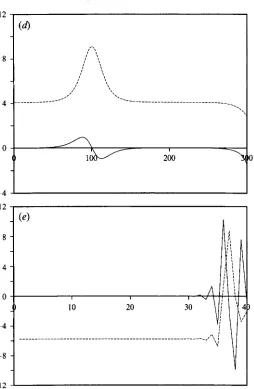
Illustrations of the stability of the periodic solutions with I =# 0 and L = 10 are shown in figure (2 c, d). The values of so are 4 log 2 and 2 log 2 respectively, of which the former satisfies (7.20). The corresponding values of Iare, from (7.7), 0.2728 and 0.5382 and in figure 2 (c) the initial values were taken as y = 0.1, S = 6,

+

0.1, but in figure 2 (d) they were y = 0.001, 8 = 8, +0.001, for the appropriate 8, from (7.8) in each case. The oscillations in figure 2(c) persist to large values of n but in figure 2 ( d ) , where (7.20) is violated, the solution does not oscillate about the appropriate values even though the initial perturbations are far smaller. A similar picture to that in figure 2(c) is obtained with so = log2, I = 0.5142, a situation in which (7.20) is again satisfied.

Figure 2(e) illustrates an example with a smaller value of L, namely L = 1. Here

so = log 2, I = 2.9722 but the inequality (7.19) is not satisfied; here the instability is due to rounding errors only. However, if so = 2log2 so that I = 2.0221, the inequality is satisfied and extremely stable oscillations (not illustrated) are obtained.

Some comment may now be made on the effect of the parameters L and I on the stability of the periodic solutions of the recurrence relations. When I = 0, only one type is stable and this requires L

>

0.6. Increasing L seems to increase the degree of stability. However, when I =k 0 this is not necessarily so as illustrated by the examples of figure 2. This is because of the complexity of condition (7.19). Increasing I does not necessarily decrease the degree of stability either, although, as stated after (7.19), there are fewer periodic solutions as only those corresponding to case (i) of (7.4) with p even are now possible.

(b) Non-periodic solutions

On vortexlwave interactions. Part 1 119 after replacing y, S by the newly calculated

7, 8.

If, at any stage, the resulting p from (7.3a) has p

>

16, then s

<

0 and the recurrence relations cannot describe a solution of the original differential equations (5.1). Indeed all solutions computed (except those that were a perturbation of case (i) in (7.4) above or of a stable situation with I =+ 0) sooner or later reached this stage and it seemed pointless to pursue them further.

The purpose of this section was to gain some feeling for what may be expected from the solutions of the differential equations (5.1). These equations have

A”=

B”

as a solution, with a sech2 profile as in (6.1). In 96 we used this solution as a basis to construct symmetric solutions in which the difference between

A”

and

B”

is small. Such solutions consist of an infinite number of humps and troughs, strictly an asymptotically large distance apart, and matching from hump to hump leads to difference equations for the relative heights and slopes of

b

and B at the top of successive humps. These equations depend on two parameters, L and N . We have analysed the periodic solutions of these difference equations, i.e. those solutions that are periodic in that they lead to equidistantly spaced humps, and have examined the stability of these solutions. We have shown that, in the case of zero cross-flow, only in one type of these periodic solutions will perturbations remain in its neighbourhood when L is sufficiently large, the other three types being unstable. With non-zero cross-flow there is one type of periodic solution, described by (7.7), (7.8) and its stability depends on both L and N .

When L 9 1 but s / L = 0(1), the difference equations may be replaced by differential equations the solutions of which suggest that in this limit all solutions of the difference equations are periodic but not with constant s. Successive values of s vary with n but after a sufficiently large n, which can be estimated from the solution of the differential equations, the sequence of values of s is repeated.

In the following section we return to the differential equations (5.1), and seek solutions in which

(b-

j ) is not necessarily small. We use the results of this section to lead to solutions in which

A”

and

B”

are periodic functions, predictions of the period being possible from the results of the asymptotic analysis.

8. Periodic solutions of equations (5.1)

The asymptotic analysis of the preceding sections with

12-

B”(

<

1 shows that in this limit periodic solutions of (5.1) exist both when the cross-flow parameter N is zero (as in (7.4)) and when it is small but non-zero (as in (7.7), L7.8)). It is reasonable to suppose that periodic solutions of (5.1) exist even when Id-BI is of order unity, and we now show, by obtaining such solutions explicitly by numerical means, that this is indeed so. These solutions are obtained by using the analytic results for small

IA”-B”I

as an initial guess, for the unknown period for example. All solutions sought will have similar symmetry to those found in 996, 7 and there is no suggestion that the study is ex- haustive. For purposes of illustration we shall usually take L = 1 except where L

+

1 is of particular interest.

We first consider the analogue of cases (i) and (ii) of (7.4). From (6.15), (6.17) and (6.19) we find that, for each, (520) reduces to h, = pn/2. Examination of (6.14) then shows that, if p is even,

A”

= B at x = t,, the base of the trough, but if p is odd then

A - B = &p, cos (h,(x- t,)/L) which, together with (6.13), implies that either

A”

or

B”

vanishes at x = t,. In cases (iii) and (iv) we obtain h, = $pn & ( y o -y,)/L respectively. In both cases (i) and (ii)

A”+

B”

is even about the trough and the hump; if p is even then

A”-

B”

is odd about the trough but is even when p is odd. Case (i) has

b-

odd about the humps while in case (ii) it is even. Cases (iii) and (iv) do not have so much symmetry although

A”+B”

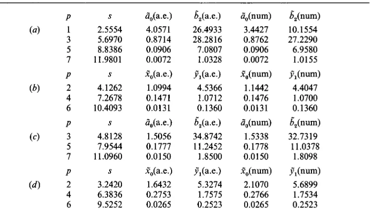
is even about both trough and hump.

120 S. N. Brown and F. T. Smith S 2.5554 5.6970 8.8386 1 1.9801 S 4.1262 7.2678 10.4093 S 4.8128 7.9544 1 1.0960 S 3.2420 6.3836 9.5252 a",,(a.e.) 4.0571 0.8714 0.0906 0.0072 Zo(a. e .)

1.0994 0.1471 0.0131 a",(a.e.) 1 SO56 0.1777 0.0150 Z,(a.e.) 1.6432 0.2753 0.0265 b,(a.e.) 26.4933 28.2816 7.0807 1.0328 y"Sa.e.) 4.5366 1.0712 0.1360 b,(a.e.) 34.8742 1 1.2452 1.8500 y",(a.e.) 5.3274 1.7575 0.2523 a",(num) 3.4427 0.8762 0.0906 0.0072 Z,(num) 1.1442 0.1476 0.0131 a",(num) 1.5338 0.1778 0.0150 fO("Um) 2.1070 0.2766 0.0265

b , ( n W 10.1554 27.2290 6.9580 1.0155 Y,(num) 4.4047 1.0700 0.1360 &(num) 32.7319 1 1.0378 1.8098 y"AnUn-4 5.6899 1.7534 0.2523

TABLE 1 (a). Case (i), p odd: predicted (cols. 3, 4) and calculated (cols. 5, 6) values of a",,

6,.

(b) Case (i)p even: predicted (cols. 3,4) and calculated (cols. 5,6) values of Z,, y",. (c) Case (ii)p odd: predicted and calculated values of a",, b,. ( d ) Case (ii) p even: predicted and calculated values of Z,,, y",.

We aim to compute the lowest modes corresponding to cases (i) and (ii) of (7.4). The eigenvalue is 2/2'/'s, the distance between the humps, and first approximations to s are given by (7.4) although strictly the formulae there hold only for s 9 1. It emerges that the lowest possible s in each situation leads to the simplest form of eigenfunction with the fewest oscillations in

2-B".

The most awkward cases to compute are those of (i) and (ii) with p odd, since then either

A"

or

B"

vanishes at the base of the trough so that (5.1) have a regular singular point. To compute the periodic solutions we first scale the equations so that the distance between trough and succeeding hump is unity. The scaling that takes the interval (0, 2-ll2s) into (0,l) and leaves (5.1) unaltered when N = 0, but replaces N by 2-l/,sN otherwise, is

(x,

2,

B",

N ) -+ (2-1/2sX, 2sP22, ~ s - ~ J , 2'/'s-'fl). _(8.1)

Integration is then initiated from the lowest point of the trough (2 = 0 say) with a target to be attained at the hump

X

= 1. The target vector is of length 2 and there are two free parameters at

X

= 0. Specifically these are, for the respective cases,

(i) target: 2(1) = J ( l ) , 2 ( 1 ) + 3 ( 1 ) = 0; (8.2a)

(ii) target:

A"'(

1) =

B(

1) = 0. (8.2b)

In both cases (i) and (ii)

2 + j

is even about the hump and in case (i)

2-3

is odd but i%eve_n in case (ii). The free parameters of

X

=-0 fQllow from the fact that in all cases

A

+

B is even about the trough, but if p is-odd

6-

is even, and conversely. If, when p

is odd, we denote the free parameters A"(O), &(O) by io,

6,

(on the assumption that it is

B"

that vanishes at the trough) then when L = 1, for small

X

-

-

121

7.5

5.0

2.5

0

-2.5

-5.0 20

15

10

5

0

-5

25

20

15 10

5

0

-5

On vortexlwave interactions. Part 1

122 S . N . Brown and F. T. Smith

1 2 3

-5

'

123

60

45

30

15

0

-15

-30

-45

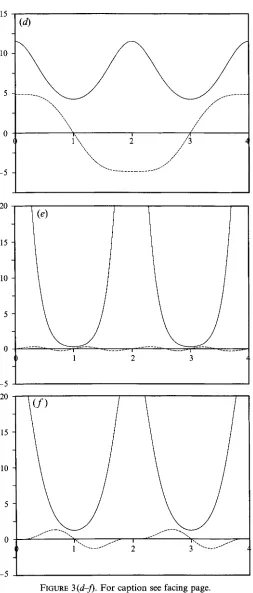
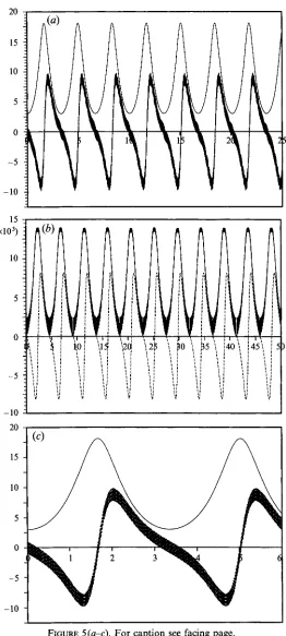
FICURF~ 3. (uk(d). The low_est periodic mode of table 1 (a-d) respectively

(I+

;continuous line,

2-3

dashed line, abs_cissa

a).

N = 0, L = 1. (e) The second periodic mode of table 1 (b) on the same scale as figu_re 3 (b). N = 0, L = 1. (f) The change from a mode of the first type to one of the second type near N = 0.075. Again L = 1. (g) An additional periodic mode with N = 0, L = 1 .

When p is even the free parameters are X,, y”, where

w w % w

2, = A”(0) (= B(0)) and y”, = A”’(0) (= (F(0)).

With L = 1 we have from tables 3 and 4 that yo = 0.0502, y1 = 0.4923. We now use cases (i) and (ii) of (7.4) to predict the values of s for the first few values ofp. This will enable the values of a“,,

h2,

X,, y”, to be predicted as initial guesses for the Newton iteration for the target in the respective cases. The predictions arcmade as follows. Once s is known, ,u follows from (7.2), and then A”(0) = ps2/2 and p(0) = p 4 / 2 from (6.13), (6.14) giving a“, and

h2

in the cases whenp is odd. Whenp is even, it follows from (6.13), (6.14) that 2, = p 2 / 4 and y”, = ,us3/4. In table 1 (a-d) we give the first few values of s, a“,,

h2,

X,, y”, as predicted by the asymptotic formulae and by the Runge-Kutta Newtonian method. Table 1 (a, b) shows case (i) with p odd and even respectively and table 1 (c, d ) shows case (ii) analogously.

We see from the table that the asymptotic formulae increase dramatically in accuracy with p and s, and %re Gseful pzedictors even at the low values of p considered here. Figure 3 (a-d) shows

A”+

B”

and A -

B”

for the smallest value of p in each of tables 1 (a)-1 (d). For convenience we have chosen to plot the figure so that 2 = 0, 2, 4 correspond to humps of the asymptotic theory while 2 = 1, 3 correspond to troughs. In figure 3 (b, c) the period is 2, and in 3 (a, d ) it is 4. The higher modes increasingly resemble the asymptotic expansion. With a period scaled to be of order unity the heights of the humps increase as s2 (see (8.1)) and theyresemble more closely sech2 profiles; in addition the number of oscillations of A - B between hump and trough increases. As an illustration of this in figure 3 (e) we plot the second mode of table 1 (b)

03 the same scale as the first mode in figure 3(b). It contains ,an

extra

oscillation of

A”-B”

between hump and trough and the maximum value of

A”+B”

is approximately 52.8.

124 S. N. Brown and F. T. Smith

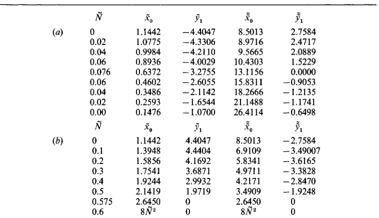
IA"-B"I

and N are small. This corresponds to type (i) with p even of (7.4), and (7.9) shows that for non-zero N there are two such solutions. In table 2(a) we illustrate the periodic solutions obtained from perturbing the leading mode in table l(b) but with

p,

= -4.407. We see that as go decreases,

fi

reaches a maximum (of 0.076) and decreases again to zero at which valug the second mode of table 1 (b) is attained. The quantities

?o,

j ,

denote the values of A and of

A",

at the hump. The change from a mode of the first type to that of the second type is illustrated in figure 3 0 in which

fi

= 0.075. This may be compared with figures 3(b) and 3(e).

A bound to

fi

is also obtained if the leading mode of table 1 (b) with

9,

= 4.4047 is perturbed. The results of so doing are shown in table 2 (b). As

8

increases 2, increases and Jl decreases until the periodic solution degenerates to

A"

=

B"

=

8fi2,

the exact solution of (5.1) noted in $5. This happens at N = 0.575. If To is increased beyond

a

value of 2.645, the hump and the trough are interchanged and

fi

decreases to zero again. The value of

fi

at which the maximum occurs can be calculated by linearly perturbing the constant solution of (5.1). The perturbations are proportional to ekiAflz where h2 = 16(1

+ad\/),

and thus are of period 2, as are those solutions we have been seeking of the nonlinear equations, when

IAIfi

is a multiple of

x.

The lowest value of

fi

from this argument is 0.57495 and at this value the solutions of the nonlinear equations reduce to linear perturbations of the constant solutions. The constant solutions exist for all values of

fi

=k 0 (and L) and can be shown to be neutrally stable, but in general the periods of the oscillations are not equal to 2. The significance of the higher values of N at which the period of small oscillations is 2 has not been investigated.

The cut-off values of

fi

evident in table 2 do not imply that periodic solutions do not exist at larger values of

fi.

The scaling properties of (5.1) result in the equivalence of a value No of

fi

and a period of 2, and a value Mo of

fi

and a period 2N0/M0. Thus as I? increases the period decreases and the amplitudes of the eigenfunctions increase

The development of the higher modes in table 2(b) as

fi

increases has not been pursued, nor is it suggested that all periodic solutions with

fi

=l= 0 may be obtained by perturbing those of case (i) of (7.4) with p even as in (7.9). The reason for success in this situation is that (5.1) are invariant under a change of sign of x provided

A"

and

B"

are also interchanged so a symmetric cross-over with

2-2

odd about both hump and trough is acceptable. The other cases of (7.4) do not have this property,

In each of tables 1 (akl (d) successive modes have an exsra zero of

A"-;

between trough and hump. 'Higher' modes also exist in which

A"+

B has a9diQonal statiogary points between trough and hump. Figure 3 (g) for example, hcs A-- B odd and A

+

B"

even about both trougb an$ hump with no additional zero of

A"-

B"

than in figure 3 (b) but a more complex A + B . In a sense it appears to be a 'second' mode, but clearly differs from that of figure 3(b). We have no analytic formula for the predictions of modes such as those of figure 3 (g) but their development with

fi

could be examined, although we shall not do so here.

The periodic solutions computed here with L = 1 may be traced as L varies. Some such solutions have been obtained in the case of N = 0. In most cases it was found that the solutions persisted as L increased but some disappeared as L decreased. For example, the simglest periodic solution, that with one oscillation of

A"-

B"

between the maxima of

A"+

B, came to an end at L2 =

$.

This phenomenon indicated the presence of multiple 'lowest mode' solutions for L2

>

+

and indeed such were found. However we shall not pursue this question of non-uniqueness.