Estimating Ocean Vector Winds and Currents Using a
Ka-band Pencil-Beam Doppler Scatterometer
Ernesto Rodríguez1*ID0000-0003-3315-4578, Alexander Wineteer1, Dragana Perkovic-Martin1,
Tamás Gál1, Bryan Stiles1, Noppasin Niamsuwan1, and Raquel Rodriguez Monje1
1 Jet Propulsion Laboratory, California Institute of Technology
* Correspondence: [email protected]; Tel.: +1-818-354-5668
Abstract: Ocean surface currents and winds are tightly coupled essential climate variables, and, 1
given their short time scales, observing them at the same time and resolution is of great interest. 2
DopplerScatt is an airborne Ka-band scatterometer that has been developed under NASA’s Instrument 3
Incubator Program (IIP) to provide a proof of concept of the feasability of measuring these variables 4
using pencil-beam scanning Doppler scatterometry. In the first half of this paper, we present 5
the Doppler scatterometer measurement and processing principles, paying particular attention 6
to deriving a complete measurement error budget. Although Doppler radars have been used for the 7
estimation of surface currents, pencil-beam Doppler Scatterometry offers challenges and opportunities 8
that require separate treatment. The calibration of the Doppler measurement to remove platform and 9
instrument biases has been a traditional challenge for Doppler systems, and we introduce several new 10
techniques to mitigate these errors when conical scanning is used. The use of Ka-band for airborne 11
Doppler scatterometry measurements is also new, and, in the second half of the paper, we examine the 12
phenomenology of the mapping from radar cross section and radial velocity measurements to winds 13
and surface currents. To this end, we present new Ka-band Geophysical Model Functions (GMF’s) 14
for winds and surface currents obtained from multiple airborne campaigns. We find that the wind 15
Ka-band GMF exhibits similar dependence to wind speed as that for Ku-band scatterometers, such as 16
QuikSCAT, albeit with much greater upwind-crosswind modulation. The surface current GMF at 17
Ka-band is significantly different from that at C-band, and, above 4.5 m/s has a weak dependence 18
on wind speed, although still dependent on wind direction. We examine the effects of Bragg-wave 19
modulation by long waves through a Modululation Transfer Function (MTF), and show that the 20
observed surface current dependence on winds is consistent with past Ka-band MTF observations. 21
Finally, we provide a preliminary validation of our geophysical retrievals, which will be expanded in 22
subsequent publications. Our results indicate that Ka-band Doppler scatterometry could be a feasible 23
method for wide-swath simultaneous measurements of winds and currents from space. 24
Keywords:surface currents; ocean vector winds; scatterometry; Doppler. 25
1. Introduction 26
The two-way interaction between ocean surface currents and ocean winds is an important 27
component of the ocean-atmosphere system. Surface winds drive currents, but are, in their turn, 28
modulated by currents since the forcing wind stress is relative to the current’s moving reference 29
frame [1]. In addition, surface currents advect warm or cold water, and the resulting temperature 30
gradients modulate the winds (e.g., [2]), possibly causing a change in the structure of mesoscale and 31
sub-mesoscale circulation (e.g., [3]). At small space and time scales, the interaction of winds and 32
surface currents becomes tighter as winds can drive inertial oscillations or aid in the formation of 33
mesoscale fronts (e.g., [4]), where significant vertical ocean motion can occur, leading to enhanced 34
mixing. For these reasons, it is very desirable to be able to obtainsimultaneoussynoptic measurements 35
of ocean surface currents and winds. 36
Measurements of ocean vector winds have a long heritage with radar scatterometers using either 37
Ku-band rotating pencil beam scatterometry (e.g. NASA’s QuikSCAT and RapidScat, ISRO’s OSCAT 38
and ScatSat) or multiple beam C-band scatterometry (e.g., EUMETSAT’s ASCAT series). The possibility 39
of measuring surface currents using radar along-track interferometry was first suggested by Goldstein 40
et al. [5,6] and an airborne vector measurement was demonstrated by [7]. Implementing a dual 41
beam along-track interferometer from space is challenging. Chapron et al. [8], with colleagues from 42
IFREMER and elsewhere, suggested that single-antenna SAR Doppler centroid measurements could 43
be used instead, albeit potentially at lower resolution and accuracy. Rodríguez (Ocean Vector Winds 44
Science Team Meeting, 2012) suggested that a slight modification of the pencil beam scatterometer 45
to include Doppler measurements could produce wide-swath vector surface current measurements, 46
and Bao et al. [9] subsequently published an analysis of the performance of a Doppler scatterometer 47
spaceborne system. Fois et al. [10] showed that a Doppler system amenable to the ASCAT architecture 48
could also be implemented by correlating the Doppler shift from opposite sense chirps. 49
Given the scientific potential for simultaneous measurements of winds and currents, NASA 50
funded the development of a Ka-band Doppler scatterometer system, called DopplerScatt, under 51
the NASA Instrument Incubator Program (IIP). Here, we present the Ka-band measurement 52
phenomenology, the processing and calibration algorithms, and the detailed detailed measurement 53
error budget for the DopplerScatt wind and current measurements. These measurements are then 54
validated using data collected in several field campaigns. 55
The DopplerScatt instrument design is presented in Section2.1. We then present a review of the 56
measurement principles and an overview of the processing in Section2.2. The measurement principles 57
are examined further in AppendixA, which extends the work of Bao et al. [9] to include several 58
additional effects. One aspect where pencil-beam Doppler centroid systems differ from side-looking 59
SAR systems is in the variation of Doppler bandwidth with scan angle [11]. This variation allows the 60
estimation of the Doppler centroid using phases from multiple bursts in order to reduce the noise of 61
the estimate. We present detailed algorithms for the estimation of the Doppler centroid that extend the 62
classical work of Madsen [12] to multiple bursts in Section2.5. We derive a new analytical estimate for 63
the radial velocity and validate it using DopplerScatt field measurements. 64
In Sections2.4-2.6, we present the description of the end-to-end processing algorithms. Given 65
the novelty of the pencil-bean Doppler measurements, we pay attention to the sensitivity equations 66
for the velocity, and validate the DopplerScatt random error performance by comparing theoretical 67
predictions and estimates obtained from campaign data. 68
DopplerScatt also differs from spaceborne scatterometers in having only one polarization and 69
one antenna beam. In traditional scatterometry, this limitation would lead to unacceptable azimuth 70
ambiguities, but we show in Section2.6that, following the spirit of Mouche et al. [13], the surface 71
current radial velocity information can be used to obtain unambiguous wind directions. 72
A critical part of the radial velocity measurement (and one of the primary limitations for 73
spaceborne SAR systems to date) is calibrating the antenna position so that the look vector is known 74
to sufficient accuracy. In Section2.8, we show that it is possible to use measurements over multiple 75
scan cycles of the pencil-beam antenna to determine angular biases and illustrate with results from 76
DopplerScatt. These results illustrate the system’s stability over multile campaigns. 77
After laying down the theoretical and processing framework, we examine in Section3 the 78
geophysical results obtained during multiple flights conducted by the DopplerScatt instrument during 79
2016 and 2017. These results include estimates of the ocean correlation times at Ka-band (Section3.1); 80
estimates of the geophysical model function (GMF) relatingσ0and winds for vertical-polarization,
81
moderate incidence angle Ka-band data (Section3.2); the separation of the ocean surface currents into 82
two components: one directly proportional to the local wind, representing the sum of Bragg wave 83
motion, Stokes and wind drift, and coupling of surface waves orbital velocities; and another one 84
corresponding to the deeper current that does not respond immedialte to the local wind (Section3.4). 85
against availablein situdata. Given the complexity of comparing radar surface velocities within
87
situmeasurements conducted by various methods, we will give a more detailed accounting of this 88
subject elsewhere. The mechanims that generate the surface current GMF through modulation of 89
Bragg waves by long ocean waves is discussed in Section4. Finally, in Sections4-5, we compare our 90
findings with similar findings obtained at different frequencies or by different measurements, and 91
assess the prospects for Ka-band Doppler scatterometry. 92
2. Materials and Methods 93
2.1. The DopplerScatt Instrument
94
DopplerScatt is a vertically polarized single-beam Ka-band coherent scatterometer using a rotating 95
pencil-beam antenna to illuminate circular regions that can be built into a continuous swath, similar 96
to the principle of the NASA’s Seawinds Instrument on QuikSCAT [14]. The 12 RPM rotation rate of 97
the antenna is set so that, for a given range, every point in the swath is observed from at least two 98
different directions, resulting in the observation geometry shown in Figure1. The data are recorded 99
coherently onboard and processed on the ground to estimate radial velocities, by using pulse-pair 100
phase differences, and normalized radar backscatter cross sections,σ0. The azimuth diversity of the
101
measurements allows for inversion of both vector surface velocities and winds, as will be explained 102
below. The antenna beam boresight is set at a nominal incidence angle of 56◦, which, at a nominal 103
flight altitude of 8.53 km, results in a ground scan radius,R, of approximately 12.5 km, for a total 104
observation swath of about 25 km. The system is highly configurable in terms of the inter-pulse period, 105
the burst repetition interval, and the system bandwidth, allowing for operation at multiple altitudes. 106
Table1presents the configuration that was used to obtain the results used in this paper. 107
f
x
f
y
R
`
ˆ
+R
`
ˆ
'
'+
Figure 1.Geometry, viewed from above, for the inversion of vector surface velocities and winds. The platform flies along thex-direction, and the cross-track distance is given byy. For a given range, the footprint scans along a circle of radiusRcentered at the radar position (indicated by a dark circle). For this simple geometry, any given point in the swath is mapped twice, with a plane-projected look vector in the forward (backward) direction given by ˆ`+k (ˆ`−k). The angleφ=arctan(2y/D) =ϕ+is the angle between the forward look and platform directions andDis the platform separation. It is related to the backward look angle byϕ− =π−φ.
A 3D model of DopplerScatt is presented in Figure2. A 5 MHz chirp signal is generated digitally, 108
upconverted, and amplified using a commercial Ka-band solid state amplifier (SSPA), built by QuinStar 109
Technology, to achieve a peak transmit power of 100 W. The signal is transmitted and received by a 110
rotating, 3◦one-way beamwidth, vertically-polarized, waveguide slotted array antenna, base-banded 111
by the RF receiver, and digitized at high rate by a commercial digital receiver built by Remote Sensing 112
Solutions. The processing of the complex data from the digital receiver will be described below. For 113
the nominal system parameters in Table1, the system achieves a noise-equivalentσ0of about -37 dB,
114
Figure 2. 3D model of the DopplerScatt system prior to integration into the radome and mounting plate installed in the belly of a King Air B200 airplane.
Although the system pulse repetition frequency allows for SAR processing, the achievable azimuth 116
resolution using SAR will vary significantly with azimuth angle, and, at this point, we have decided 117
to process the data in real-aperture mode to obtain more uniform sampling characteristics. This 118
leads to a two-way azimuth footprint size of approximately 600 m. In the range direction, the chirp 119
bandwidth results in a ground sample spacing of 36 m. The achievable ground resolution when 120
combining multiple looks for different directions will vary across the swath, but can lead to significant 121
improvements in the resolution cell size, especially in the swath “sweet-spots” between the nadir track 122
and the far-swath [15]. 123
Pulsed pair Doppler processing is achieved by cross-correlating bursts which are transmitted at a 124
burst repetition frequency of 4.5 kHz, Nyquist oversampling the Doppler bandwidth for all azimuth 125
angles. The system’s phase and power stability is monitored a using an internal calibration loop which 126
includes the transmit and receive paths, excluding the rotating antenna. Intensive laboratory testing 127
prior to deployment, and subsequent calibration field data, showed that the pulse-pair difference 128
timing stability is insensitive to temperature and introduces radial velocity errors much smaller than 129
1 cm/s. The system delay showed some sensitivity to temperature, but drifts were much smaller than 130
the inverse bandwidth of the system. The system gain exhibited variations with temperature and these 131
were calibrated using loop-back calibration and corrected during the processing to obtainσ0.
132
The instrument position and attitude are obtained using a GPS receiver coupled with an 133
Applanix POS AV-610 Internal Motion Unit (IMU). The IMU manufacturer specifications1relevant to 134
DopplerScatt’s performance are given in Table2, assuming Precise Point Positioning (PPP)2processing. 135
The rotation angle is obtained by means of an encoder, which has a nominal resolution of 88 mdeg, but 136
has an unknown mounting offset that needs to be obtained from calibration. The nominal antenna 137
pattern was obtained using near-range field measurements. The nominal boresight was obtained by 138
combining mechanical measurements of the antenna location together with IMU attitudes and the 139
azimuth encoder measurement. 140
2.2. Current Measurement Principle
141
DopplerScatt measures two basic quantities, pulse-pair phase differences and return power, which 142
are then converted to surface radial velocities,vrS, and normalized backscatter cross section,σ0. The
143
use ofσ0for vector wind retrieval using a pencil-beam scatterometer is well known (e.g., [16]), and we
144
Table 1.DopplerScatt nominal parameters.
Parameter Value
Peak Power 100 W
3 dB Azimuth Beamwidth 3◦ 3 dB Azimuth Footprint 600 m 3 dB Elevation Beamwidth 3◦
3 dB Elevation Footprint 1.4 km Nominal boresight angle 56◦ Burst Repetition Frequency 4.5 kHz
Inter-pulse Period 18.4µsec Chirp length 6.4µsec Pulses per burst 4 Pulse Bandwidth 5 MHz
Azimuth Looks 100
Range Resolution 30 m Resolution in Elevation 36.2 m
Resolution in Azimuth 485 m Nominal Platform Altitude 8.53 km
Nominal Swath 25 km
Scan Rate 12 RPM
Noise Equivalentσ0 -37 dB
Table 2.Applanix POS AV 610 performance specifications.
Parameter Accuracy True Heading 5 mdeg
Roll & Pitch 2.5 mdeg Attitude Drift <0.01 deg/hr
Velocity 0.5 cm/s Horizontal Position <10 cm
Vertical Position <20 cm
refer the reader to the literature for a review of the principles. The principles of using a pencil-beam 145
system to measure surface currents was presented by Bao et al. [9]. In this paper, we extend their 146
derivation to include various effects not accounted for in their first order approximation and also 147
examine the algorithm for radial velocity in detail. 148
In AppendixA, we present a detailed measurement model and find that the complex correlation 149
coefficient,γ(τ), for a pulse pair separated by a timeτis given by 150
hE1E∗2i r
D
|E1|2E D|E2|2E
≡γ(τ) =exp[−iΦ(τ)]γNγT(τ)|γD(τ)| (1)
Φ 2kτ =
ˆ
`·
vp−
vW+
δσ0
σ0
ˆ
`·δvW
W
−vrG−vrA (2)
whereEi is the complex return signal,Φis the pulse-pair phase difference, 2kτ =4πτ/λ, ˆ`is 151
the look vector from the platform to the scattering cell3,vpis the platform velocity vector, andvW
152
is the velocity vector for the surface scatterers averaged over the resolution cell. Equation (2) shows 153
that the normalized pulse-pair phase is proportional to the radial velocity along the look direction, 154
ˆ
`· vp−vW, as in [9], but also includes three additional terms.
155
The first term,Dδσ0 σ0
ˆ
`·δvW
E
W, represents the correlation betweenσ0andvWfluctuations within
156
the resolution cell, reflects the modulation of the resolution cell Doppler centroid by changes in 157
σ0. Thus, if velocity and back scatter modulations are correlated (by hydrodynamic, tilt, or other
158
modulations), the radial velocity contributing to the Doppler will not be ˆ`·vW, but will be shifted
159
towards the velocities in the brighter parts of the long waves and may cause a net Doppler shift even 160
when the average wave orbital velocity is negligible. The presence of this coupling was first shown by 161
Chapron et al. [8], and has been incorporated subsequently into the DopRIM model [17–19]. This type 162
of modulation has been shown to be important at C-band [8,18] and X-band [20], and to introduce a 163
significant wind component which is a function of both wind speed and direction, with theory being 164
in general good agreement with observations. At Ka-band, there is a much smaller literature, although 165
recently Yurovsky and colleagues [21,22] have shown empirical and theoretical evidence for a wind 166
induced component, which will be discussed in greater detail below. 167
The second term, vrG, is due to shifts in the Doppler centroid caused by non-random (i.e.,
168
non-wave-related) variations in the backscatter cross section over the resolution cell, such as those 169
due to a gradient in wind speed, or aσ0variation due to surfactants. A detailed derivation of the
170
magnitude of this term is given in AppendixA. When the antenna pattern is well approximated by a 171
Gaussian, as is the case for DopplerScatt, the term is well approximated by 172
vrG =
∆
σ0
σ0
σφa
vpsinφ (3)
where∆σ0is the change inσ0over the footprint, σφa ≈ 0.02 is the standard deviation of the
173
azimuth beamwidth, andφis the azimuth angle relative to the velocity direction. For a 0.1 dB variation 174
over the ∼ 600 m azimuth footprint, corresponding roughly to a 10 cm/s change, and a nominal 175
platform velocity of 130 m/s, this corresponds to a maximum error of about 6 cm/s at broadside, while 176
the average error over the swath is significantly smaller. This error can increase substantially in the 177
presence of sharpσ0discontinuities, and must be corrected in the processing if the discontinuity is
178
large enough using the measuredσ0data.
179
The final term, vrA, is due to shifts in Doppler centroid due to asymmetry in the antenna
180
pattern, and, if large enough, must be corrected in the processing by using antenna pattern calibration 181
measurements. 182
The magnitude of the pulse-pair correlation,γ, determines the noise in the estimated pulse-pair 183
phase difference and contains contributions from three distinct mechanisms. The first term, γN =
184
SNR/(1+SNR), whereSNRis the system signal to noise ratio, is the use term induced by the presence 185
of random thermal noise. Given the small noise-equivalentσ0for DopplerScatt, it only plays a role
186
for very low wind speeds. The next term,γT, is due to changes in scatterer phase due to surface
187
motion between the pulses used to form the pulse-pair phase. This temporal correlation is the product 188
ofγTS, due to the finite lifetime of surface scatterers, andγTW, due to scatterer motion induced by
189
long-wavelength surface waves 190
γTW(τ) =exp " − τ TW 2# (4)
TW=
√
2kσWr
−1
(5)
whereTWis the correlation time due to wave motion, andσWris the standard deviation of the
191
wave orbital velocity along the radial direction. Although an upgrade is planned, DopplerScatt does 192
not have the capability to resolve surfaces waves currently, so an estimate of the orbital radial velocity 193
variance cannot be obtained from the data itself, but it can be obtained usingin situknowledge of the 194
surface wave spectrum or by assuming that its is purely wind-driven and has reached equilibrium 195
with the wind. The termγTSis due to non-linear dissipation of resonant scatterers or wave breaking,
Figure 3. Observed (solid lines) and modeled (dashed lines) pulse-pair correlations for pulse-pair separationsτ =nτ0,τ0 = 0.22 msec, as a function ofφ, the azimuth angle relative to the platform velocity.
for which we do not have appropriate models at this time. However, the temporal correlation term can 197
be estimated from the data itself, as we will show below. 198
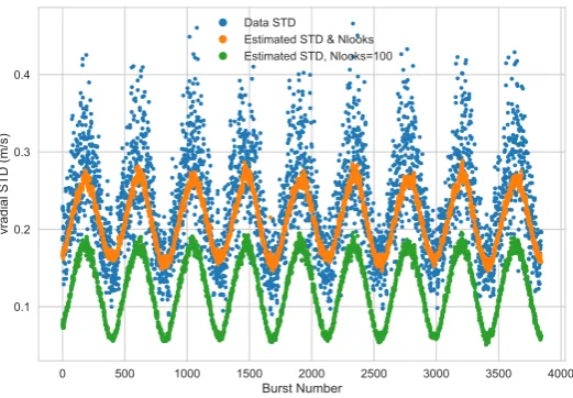
The final term contribution to signal decorrelation,γD, is due to the variation of the Doppler shifts
199
within the resolution cell, and is given by the Fourier transform of the resolution cell illumination 200
at the Doppler shift spatial fringe rate, equation (A27). For a Gaussian antenna pattern and range 201
resolution that is small compared to the changes in Doppler in the range direction, this term can be 202
approximated by 203
γD ≈exp
" −
τ
TD
2 sin2φ
#
(6)
TD =
√
2kvpσφa −1
(7)
whereTDis the Doppler decorrelation time at broadside, which is on the order of 0.35 msec.γD
204
reaches a maximum in the fore and aft directions, and a minimum at broadside. Notice thatTD/TW =
205
σWr/vpσφa1, since we find in Section3that the typical ocean correlation timeTW &2 msec. The
206
Doppler term dominates the correlation for about 80% of the swath, but, due to the sin2φterm, the 207
surface temporal correlation is dominant for the inner 20%. 208
To test the validity of the correlation model, we estimate the pulse-pair correlations as a function 209
ofτandφfrom collected data correlations and compare against predictions for the DopplerScatt 210
parameters assuming a Gaussian antenna pattern. A typical result is shown in Figure3, where observed 211
correlations (solid lines) estimated using 100 pulse pairs for a 200 km line of data are plotted against 212
the theoretical prediction in equation (6) for three different pulse-pair separations given byτ=nτ0for
213
n=1, 2, 3 and burst-repetition intervalτ0= (4.5 kHz)−1≈0.22 msec. Since the temporal correlation
214
is unknown, it is fit for each pulse-pair interval by making the theoretical and observed curves match 215
in the aft direction,φ = 0. These estimates will be used to estimate ocean correlation times in the 216
results section below. 217
Several features of the DopplerScatt signal are apparent from Figure3, in addition to the good 218
agreement between theory and observations (the deviations for low correlation values are due to biases 219
in the correlation estimator, and the two curves agree for moderate to large values ofγ). As expected, 220
the correlation is inversely proportional to the Doppler bandwidth, withγD≈1 in the fore (φ=π) 221
and aft (φ = 0), while the correlation is minimized at broadside (φ = ±π/2). Thus, it is expected 222
fore and aft. The second lesson from this figure is that temporal correlation of the signal can be a 224
significant contributor to signal decorrelation. The variability of the ocean temporal correlation times 225
as a function of environmental conditions will be examined below. 226
2.3. Estimation of Pulse-Pair Phase
227
Traditionally, the estimation of phase differences for Doppler centroids [12] and radar 228
interferometry [23], for pulses separated byjτB(j≥1 is an integer), whereτBis the burst repetition
229
interval, has been done by using the phase of the pulse-pair interferogram 230
ˆ Φj =
1
j arg
"Np
∑
n=1
D
En(t)E∗n+j(t+jτB)
E #
(8)
where the indexnlabels subsequent pulses in the received pulse train. Following Madsen [12], 231
in SAR applications j = 1, since typically pulses separated by more than one can be regarded as 232
uncorrelated. This can be shown to be the maximum likelihood estimator (MLE) for the interferometric 233
phase when usingindependentpulse pairs, but not when the pulses are not independent. As can be seen 234
from Figure3, pulses in the DopplerScatt return may have significant correlation across many transmit 235
events and a natural question arises on what the best combination of pulse pairs should be used to 236
estimate the pulse-pair phase. In AppendixB, we present the derivation of the MLE estimator for 237
the pulse-pair phase difference, as well as the Crámer-Rao asymptotic lower bound for the estimator 238
variance [24]. Unfortunately, unlike for the independent pulse-pair samples, the MLE equation (A42) 239
does not have an analytic solution, bust must be solved numerically by a one-dimensional search, 240
or by iteration, which has a computational cost. In the low-correlation limit, the estimator can be 241
approximated by the weighted average of the MLE estimator 242
ˆ
Φ=
Nj
∑
j=1
wjΦˆj (9)
wherewjis an approximate inverse variance weight given by equation (A53).
243
For independent pulse pairs with the same correlationγ, the Cramér-Rao bound is given by [23] 244
σΦ2 = 1 2NL
1−γ2
γ2 (10)
whereNL is the number ofindependentpulse pairs used in the estimate. When the pulses are
245
correlated, the Cramér-Rao bound is given by equation (A47), which can be calculated analytically 246
but does not lend itself to a simple expression, except in the low-correlation limit when it is given by 247
equation (A50), which represents a weighted combination of equation (10) accounting for changes in 248
the number of samples and correlations. 249
To assess the relative performances of the estimation algorithms we generated correlated 250
circular-Gaussian samples with the correlation coefficient given by equation (1), using a Gaussian 251
antenna pattern. The temporal correlation function was assumed to be of the form γT =
252
exp[−(τ/Tsc)2]andTscwas varied between 0.5 msec to 4.0 msec, consistent with ocean observations
253
presented below. We examine three estimators: the MLE estimator; and the two estimators obtained 254
by takingNj =1, 3 in equation (9). TheNj =1 case corresponds to the Doppler centroid estimator
255
given by Madsen [12] and has correlations similar to then=1 line in Figure3(although with varying 256
temporal correlation). TheNj =3 estimator uses the three pulses shown in Figure3. For this simulation,
257
we use 100 pulses (as in the processor) and the nominal system parameters in Table1. The results for 258
0.0 0.2 0.4 0.6 0.8 1.0
Normalized Cross-Track Distance
0 10 20 30 40 50
Radial Velocity STD (cm/s)
Madsen Estimator
T
c: 0.5 msecT
c: 1.0 msecT
c: 2.0 msecT
c: 4.0 msec0.0 0.2 0.4 0.6 0.8 1.0
Normalized Cross-Track Distance
0 10 20 30 40 50
Radial Velocity STD (cm/s)
Weighted Madsen, k=3 Estimator
0.0 0.2 0.4 0.6 0.8 1.0
Normalized Cross-Track Distance
0 10 20 30 40 50
Radial Velocity STD (cm/s)
MLE Estimator
Figure 4.Performance of three pulse-pair estimators described in the text as a function of cross-track distance divided by the swath radius=|sinφ|. Solid lines correspond to the Cramér-Rao bound given by equation (A47). Circles correspond to the simulation results as a function of correlation time forTc of 0.5 msec (blue), 1.0 msec (green), 2.0 msec (red), and 4.0 msec (purple).
Figure4shows the radial velocity error increasing with cross-track distance for all estimators, and 260
decreasing with increasing correlation time. Surprisingly, the best estimator is the Madsen estimator 261
(Nj=1), while taking additional samples (Nj =3) increases the noise, as does using the MLE solution
262
(possibly due to errors in the numerical search). These characteristics hold for high SNR data where 263
reducing thermal noise variability is not important, while lower SNR results (not shown), that will be 264
more representative of spaceborne data, do show the benefit of using multiple samples in the retrievals. 265
The reason the Madsen-type estimators do not conform to the approximate Cramér-Rao bounds is 266
that they utilize the number of pulses used to form the interferogram,Np, as the number of independent
267
looks,NL, in equation (10). This is appropriate only in the limit when pulse-to-pulse correlation is
268
low, as derived in AppendixB. However, when pulse-to-pulse correlation is high,NL Np. A better
269
total correlation time,NL=NpτB/Tc,Tcis determined by solving|γ(Tc)|=1/e. From equations (4)
271
and (6),Tcis given by
272
Tc=T
q
1+log(γN) (11)
T−2=hTW−2+TD−2sin2φ i
(12)
SinceTD TW, for about 80% of the swathT−1varies sinusoidally with azimuth angle (or
273
linearly with cross-track distance), but approaches a fixed value determined by the ocean correlation 274
time in the nadir portion of the swath. For logγN >−1, the equivalent number of looks can be written
275
as 276
NL =min
NpτB
q
TW−2+TD−2sin2φ p
1+log(γN)
,Np
(13)
In the high-correlation limit, 1−γ1, which applies in most situations for DopplerScatt, one 277
can use the Cramér-Rao bound to derive a simple formula for the radial velocity error variance 278
σvr2 =
1 2kτB
2 1 2NL
1−γ2
γ2 (14)
≈
1 2kτB
2 τB
Np
q
TW−2+TD−2sin2φ (15)
which shows that for about 80% of the swath, the radial velocityvariancewill varylinearlywith 279
cross-track distance and approach a fixed value for the center swath. If the effect of the equivalent 280
number of looks were not taken into account, the prediction would be that the radial velocity variance 281
would exhibit aquadraticbehavior with cross-track distance, in the high correlation limit. This equation 282
also shows thatσvr2 ∼τB−1, rather than theτB−2behavior that would be expected if the phase variance 283
were independent of the pulse-pair separation. 284
In Figure5, we show the expected random error performance as a function of SNR and ocean 285
temporal correlation using the exact correlations and estimated number of looks. For SNR greater 286
than 20 dB, the high correlation behavior described above applies, but the performance across the 287
swath flattens out significantly as the SNR becomes smaller, since the performance is dominated by 288
the thermal noise and not the Doppler correlation. The impact of ocean correlation time is only evident 289
in the nadir part of the swath and for lower SNRs. 290
In Figure6, we compare the estimated noise in the radial velocity (blue), against predictions using 291
equation (10) with the estimatedγusing either the naïve Cramér-Rao bound (NL = Np) (green), or
292
the version whereNLis estimated from the total correlation time (orange). The estimates of the radial
293
velocity random error (blue) were obtained for each pulse-pair by removing a trend in range for the 294
radial velocity and computing the standard deviation of the resulting signal: this is a conservative 295
estimate since there will be some natural variability due to waves and currents. Since the ocean 296
surface correlation time is unknowna priori, we estimate theγN and Tc by fitting a quadratic in
297
time for multiple pulse separations to the logarithm of the correlation function and averaging the 298
estimates for each range line for the same samples used to estimate the random error (additional results 299
regarding the temporal correlation function are given in Section3.1). Both measured and predicted 300
random errors show periodic variations with azimuth due to the changes to predicted the Doppler 301
correlation in equation (6), with minimum errors occurring in the fore and aft directions, and maxima 302
at broadside. The figure shows that the naïve estimator underestimates the observed error significantly, 303
while the Cramér-Rao bound withNLdetermined by the correlation time is in good agreement with
Figure 5. Random component of the radial velocity for SNRs of 5 dB (blue), 10 dB (orange), 20 dB (green) and 30 dB (red) and radial velocity standard deviations (0.2 m/s (solid), 0.4 m/s (dashed), and 0.6 m/s (dot-dashed) for a platform velocity of 130 m/s and assuming thatNp=100 andτ≈0.2 msec. The cross-track distance is divided by the distance from the nadir track to the outer swath.
the observations. The fact that the naïve estimator underestimates the error significantly explains 305
the degraded performance when multiple pulses are used in combination using equation (9): the 306
estimation weightswjare too large for the larger pulse-pair separations, resulting in the introduction
307
of additional noise. One can improve the multi-pulse estimator in equation (9) by using the predicted 308
variances which incorporate the effective number of looks into the weights,wj, but we have found that
309
this modification has only small effect on the estimation, due to the larger errors for greater pulse-pair 310
separation. At this point, we do not have a simple explanation why the MLE estimator performs so 311
poorly against the pulse-pair interferogram phase. 312
2.4. Processing toσ0and radial velocities
313
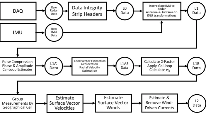
Figure7presents an overview of the DopplerScatt data processing, which, following the usual 314
NASA conventions, produces data at three different levels: Level-0 (L0) data transformed from 315
raw digital subsystem (DAQ) and IMU data into quality-assessed engineering radar and IMU 316
data in physical units; Level-1 (L1) data produces geolocated estimates of σ0 and residual radial
317
velocity, after subtracting platform motion effects, obtained by combining 100 transmit pulses; 318
Level-2 (L2) data contains geolocated estimates for surface vector winds and currents sampled along 319
individual observations swaths. Level-3 gridded data is obtained by combining multiple swaths 320
and requires accounting for temporal differences between different swaths, which typically requires 321
some assumption about dynamics, and is not an official product at this point given uncertainties in 322
the dynamics at DopplerScatt resolution scales. Below, we describe the general interest L1 and L2 323
processing algorithms, as L0 processing is hardware specific. 324
The DopplerScatt instrument uses four different coordinate systems to go from raw measurements 325
to geolocated data: a system intrinsic to the antenna; a system fixed relative to the instrument mounting 326
plate; a system relative to the aircraft; and, finally, the East-North-Up (ENU) geolocated coordinate 327
system. In the early part of L1 processing, GPS/IMU data are merged with the time-tagged radar 328
data and transformation matrices between the coordinate systems are derived. The down-converted 329
0 500 1000 1500 2000 2500 3000 3500 4000
Burst Number
0.1 0.2 0.3 0.4
vradial STD (m/s)
Data STD
Estimated STD & Nlooks Estimated STD, Nlooks=100
Figure 6. Estimates of radial velocity random error obtained from observations (blue), using equation (10) (divided by 2kτ) withNL=Np(green), and using the same equation but estimatingNL from the correlation timeTc(orange). The data shown corresponds to 4.5 revolutions of the antenna. Note the variations in random error as a function of azimuth due to the variations inγD(φ), with error maxima appearing at broadside, as predicted by equation (6).
convolution using a weighted reference chirp, to reduce range sidelobes. Estimates of both the phase 331
and amplitude of the loop-back chirps are calculated and stored for data processing. 332
A critical part of the processing is in the estimation of ˆ`, the vector along the look direction, which 333
is given in the ENU system by 334
ˆ
`=sinθ[nˆcosα+eˆsinα]−uˆcosθ (16)
where ˆn, ˆe, ˆuare unit vectors pointing north, east and up, respectively;θis the look angle; andα 335
is the azimuth angle measured clock-wise relative to north. 336
Assuming a local spherical Earth approximation with radius of curvatureRE, the look angle to
337
the center of the range pixel can be written in terms of the range,r, the height of the platform above 338
the WGS84 ellipsoid from the GPS measurements,h, and the surface height,η, which is assumed to be 339
constant over the resolution cell: 340
cosθ= h−η
r +
(r/(RE+η))2−((h−η)/(RE+η))2
2(r/(RE+η)) (1+ ((h−η)/(RE+η))) (17) The range term has precision comparable to the system timing, which is much better than the 341
precision in the height above the surfaceη, obtained using the CNES-CLS11 mean sea surface [25]. 342
Neglecting curvature terms, the error in the look angle is given by 343
δθ≈ δ(h−η)
rsinθ (18)
Using the nominal DopplerScatt parameters, and assuming that the coupled IMU-GPS and 344
knowledge of the ocean surface are known to within 10 cm, the error in the look angle will be on 345
the order of 6.6µrad ∼ 4×10⁻⁴deg, which will cause minimal errors on velocity estimation and 346
DAQ IMU Raw Radar Data Raw IMU Data Data Integrity
Strip Headers DataL0
Interpolate IMU to Radar Antenna & Airframe to
ENU transformations
L1 Data
Pulse Compression Phase & Amplitude Cal-Loop Estimates
L1A’ Data
Look Vector Estimation Geolocation Radial Velocity Estimation L1AS Data Calculate X-Factor Apply Cal-loop
Calculate s0
L1B Data Group Measurements by Geographical Cell L2 Data Estimate Surface Vector Velocities Estimate Surface Vector Winds Estimate & Remove Wind-Driven Currents
Figure 7.End-to-end flow of the DopplerScatt processor.
Following AppendixA, the azimuth angle must be estimated as the mean value over the footprint 348
weighted by the antenna pattern and brightness. We assume constant brightness over the footprint 349
and compute the mean value as 350
α=
R
dα0G2(θ,α0)α0
R
dα0G2(θ,α0) (19)
whereG2is the two-way gain mapped into elevation and azimuth coordinates, and, given the
351
small angular size of the range pixel, integrate along an iso-θcut in the elevation direction. αcan 352
be in error due to errors in the measured antenna pattern or due to coupling between the odd parts 353
of the antenna pattern and brightness gradients. These effects are much smaller in practice than the 354
errors that can be caused by a systematic offset,δα, between the antenna azimuth encoder and the 355
IMU. Below, we discuss how this mounting offset can be estimated during the calibration process. 356
Once the look vector is estimated, the scatterer position,S,is determined in the ENU coordinate 357
system usingS=P+r`ˆ, whereP is the nominal radar phase center position from the GPS/IMU. 358
Geolocation into latitude and longitude from ENU is then performed for each pulse. 359
To estimate the surface velocity, pulse-pair phase differences are computed using 100 contiguous 360
bursts, and the platform motion effects are removed by multiplying by a term exph2ikjτ`ˆ0·v0p i
, 361
where ˆ`0 andv0
p are the estimated look vector and IMU/GPS platform velocity, respectively. This
362
process of interferogram flattening also ensures that the residual phase does not suffer from phase-wrap 363
ambiguities. After estimating the flattened interferometric phase,δΦˆ, using the estimator in equation (9) 364
(Nj=1 or 3 are both kept), the raw surface-projected radial velocity,v0rS, is estimated using the equation
365
v0rS=
1 sinθ
δΦˆ 2kτ =
1 sinθ
Φˆ
2kτ− ˆ
`0·v0 p
(20)
At this point, the radial velocity contains potential calibration errors, as well as contributions from 366
not only surface currents but also the velocity of the scatterers due to Bragg wave motion, differential 367
brightness due to long-wave modulation, Stokes and wind drift effects. The final radial velocity, 368
vrS, removes these effects by subtracting a calibration term,FC, and (optionally) a surface current
369
geophysical model function (GMF) termFS
370
Section2.7discussesFC, whileFSis discussed in Section3. We refer to the radial velocity without
371
FScorrection as theuncorrectedradial velocity.
372
The backscatter cross sectionσ0is computed from the multi-looked received power,Pr, by using
373
the equation 374
Pr =Ptσ0LX (22)
X(r) = λ
2
(4π)3
∆r r3
Z
dα0G2 θ,α0 (23)
wherePtis the transmit power,Lis the system loss outside the calibration loop, and∆ris the
375
range resolution. In the equation for theX−factor, we have assumed that the integral along the range 376
direction of the range point target response,χ2, is given by∆r=R dr0χ2(r0−r). The same 100 pulses 377
are used for computing the multi-looked power as the for the interferograms. 378
2.5. Estimating the Surface Velocities and Errors
379
The DopplerScatt rotating pencil-beam illuminates a swath of width 2R=2hsinθ(see Figure1), 380
where h is the platform height above the surface and θ is the look angle. For a given range (or 381
look angle), every point in the swath is imaged twice, looking forward and back, respectively. Using 382
equation (21), estimates forv+/rS −, the radial velocities projected on the horizontal plane can be obtained 383
after removing the platform velocity contribution to the pulse pair phase. The radial velocities are 384
defined by 385
v+/rS −=vS·`ˆ+/k −= vS·
ˆ
`+/−
sinθ (24)
where ˆ`+/−is the look vector from the radar to the scattering point; they are related tovx/y, the
386
surface velocities along thex/ydirections, respectively, by 387
cosφ sinφ −cosφ sinφ
!
vx
vy
!
= v
+
rS
v−rS
!
sinφ= y
R
whereφ = ϕ+ is the forward-look azimuth angle shown in Figure1. It is related to ϕ−, the 388
back-look azimuth angle, byϕ−=π−φ. 389
Separating explicitly the measured radial velocities and the velocity GMF, this equation can be 390
inverted 391
vx
vy
!
= 1
sin 2φ
sinφ −sinφ cosφ cosφ
!
vrS0+−FS+ vrS0−−FS−
!
(25)
so that the surface components can be retrieved everywhere, with the exception of along the nadir 392
path (φ=0) for they-component, or at the edge of the swath (φ=π/2) for thex-component, when the 393
inverse matrix is singular. 394
In practice, due to the finite beamwidth of the antenna and finite cell size of the retrieval, a given 395
point in the ground can be imaged multiple times, and the surface currents are inverted by weighted 396
least-squares inversion. However, for the purpose of calculating the measurement sensitivities, these 397
simplified equations are sufficient to illustrate the nature and magnitude of the errors, provided random 398
measurement errors are adjusted for the appropriate number of looks. The sensitivity equations are 399
δvx=
δv0rS+−δv0rS− 2 cosφ −
δ FS+−FS−
2 cosφ (26)
δvy=
δv0rS++δv0rS− 2 sinφ −
δ FS++FS−
2 sinφ (27)
These equations show that the surface velocity errors are a function of cross-track distance,y, 401
but not of the along-track coordinate,x, with unbounded errors at the nadir and far swath. They 402
also indicate that we can expect the along-track error to be large at the edges of the swath, while the 403
cross-track errors will grow in the nadir direction. Finally, they show that, if the radial velocity errors 404
are symmetric with respect to look direction (i.e.,δv+rS =δv−rS), then the along-track velocity errors 405
cancel, whereas, if they are antisymmetric (i.e.,δv+rS=−δvrS−), the cross-track errors cancel. 406
Aside from geophysical effects inFS, the DopplerScatt surface velocity error budget is dominated
407
by two types of errors: random noise which is caused by thermal noise, speckle, and temporal 408
decorrelation; and errors due to incorrect removal of the platform Doppler velocity from the radial 409
velocity. Assuming that the fore and aft random velocity errors are not correlated, the random error 410
standard deviations will be given by 411
σvx = q
σvrS2 ++σvrS2 −
2 cosφ ≈
σvrS
√ 2 cosφ
(28)
σvy = q
σvrS2 ++σvrS2 −
2 sinφ ≈
σvrS
√ 2 sinφ
(29)
where σvrS2 +/− is the radial velocity random variance for the fore/aft directions using 412
equations (14). The last approximation follows in the high SNR limit, when theσ0variations due to
413
different azimuth look angles can be ignored as a contributor to the total pulse to pulse correlation, so 414
thatσvrS2 +≈σvrS2 −. 415
The previous formulas apply for estimates obtained by combining pairs of radial velocity 416
measurements. In practice, we combine all fore and aft radial velocity measurements whose centers 417
lie in a finite resolution cell small enough so that the azimuth angle can be taken to be constant. This 418
allows us to reduce the random measurement noise by the square root of the number of independent 419
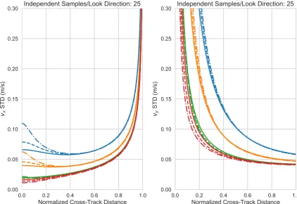
fore and aft measurements that lie within the resolution cell. Figure8shows the theoretical predicted 420
random error performance as a function of SNR and correlation time for a 200 m resolution cell, which 421
corresponds to approximately 25 independent fore and aft radial velocity estimates. Combining 422
multiple radial velocities from similar look directions also allows for an independent estimate of the 423
random component of the error and the associated estimated standard error, as shown in Figure9. 424
Using equations (28) and (29), these standard errors can be propagated to the along and cross-track 425
error estimates (see Figure10), which show good agreement with the theoretical results in Figure8. 426
In addition to the random measurement error, the other major source of instrument-related errors 427
is the subtraction of the platform radial velocity contribution, which can suffer from errors in the 428
estimated platform velocity, as well as look and azimuth angle estimation. Of these, the azimuth angle 429
estimation is dominant for a mechanically scanned antenna, since knowledge of the azimuth angle is 430
dependent on the encoder accuracy of the reported the antenna scan angle. In this case, the associated 431
radial velocity error will be given by 432
ra
d
ia
l
v
e
lo
c
it
y
s
ta
n
d
a
rd
e
rr
o
r
(c
m
/s
)
y
x
2
5
k
m
100 km
20.017.515.0 12.5
10.0 7.5 5.0 2.5 0.0
Figure 9.Estimated standard error of the radial velocity for fore-looking angles (aft-looking results are similar) obtained by dividing the standard deviation of fore-looking radial velocities in 200 m boxes, divided the square root of the number of independent samples (∼25).
where, as shown in Figure1,ϕis the relative angle between the platform velocity and the look 433
direction. Sinceϕ− =π−ϕ+, one will haveδv+rS=δv−rSas long as the azimuth error remains constant 434
between fore and aft observations. Replacing this in equations (26) and (27), one sees that a constant 435
azimuth bias will affect the cross-track surface current, but will have little impact on the along-track 436
component. An error in the along-track component due to a constant azimuth bias will introduce a 437
constant cross-track bias 438
δvy=vpkδϕ (31)
This equation shows the great sensitivity of the cross-track component to azimuth errors. For 439
example, to get to a velocity error of 10 cm/s assuming a platform velocity of 100 m/s, one must 440
require thatδφ≤10−4≈0.006◦, which can present a significant installation challenge. 441
In practice, we expect errors in the azimuth angle to have two main sources: 1) a constant bias 442
due to a mismatch between the antenna spin mechanism coordinate system; and, 2) periodic changes 443
in rotation speed due to changes in friction as the antenna spins. This leads us to assume that azimuth 444
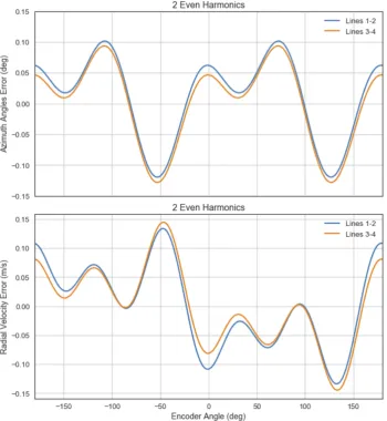
estimation error will be of the form 445
δϕ(η) =δϕ0+
Nh
∑
n=1
[ancos(nη) +bnsin(nη)] (32)
whereηis the antenna encoder angle, which, for nominal flight conditions will be approximately 446
ϕ, but will be offset by a constant when cross-winds induce a difference between the flight direction 447
and the airplane forward direction. Following the previous argument, the cross-track surface velocity 448
component will be most sensitive to terms inδϕwhich do not change sign whenη+ →η−, while the 449
along-track component will be sensitive to those harmonics that do change sign. 450
The final source of surface velocity errors is due to errors in the wind-driven radial velocity 451
contribution,FS. In Section3.4, we show thatFSis well represented by a low-order harmonic expansion
452
FS(ϕ,U10,ϕU) =δvr(U10) + NS
∑
n=1
vrn(U10)cos(n(ϕ−ϕU+δϕ(U10))) (33) whereU10is the neutral wind speed measured at 10 m;ϕUis the wind azimuth direction; andδvr,
453
vrn, andδϕare the wind speed dependent model parameters up to orderNS. In practice, the dominant
454
terms are the first harmonic (n=1) and, to a lesser extent, the constant term. TheFSassociated errors,
455
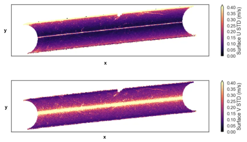
Figure 10.Estimated along-track (upper) and cross-track (lower) surface velocity component errors, obtained by propagating radial velocity standard errors, as in Figure9. Note the agreement with theoretical estimates shown in Figure8for high SNR situations.
δvx=−δ(vr1cosϕU+2vr2sinφsinϕU) (34)
δvy=−δ(δvr+vr2cos 2ϕU)
sinφ −δ(vr1sinϕU−2vr2sinφcos 2ϕU) (35) Then = 1 term in FSis equivalent to a current along the wind direction, and errors result in
457
a two-dimensional current error vector, −δ(vr1cosϕU,vr1sinϕU). As shown in Section3.4,vr1is
458
relatively constant for most of the wind speed range and is about 0.75 m/s, so that, in practice, the 459
major error contribution from the first order term will be through errors in the estimated wind direction, 460
resulting in an error vectorvr1(sinϕU,−cosϕU)δϕU, whose magnitude isvr1δϕU. The effect of a
461
wind direction error will be to add an approximately constant magnitude surface current vector in the 462
directionorthogonalto the wind direction, whose scale of variability will be the spatial scale of wind 463
direction change. Given the magnitude ofvr1, the wind azimuth angle estimation will play a dominant
464
role in the subtraction of the wind-driven surface current components, but not in their derivatives, 465
since the wind direction varies much more slowly than the ocean circulation direction. Thevr1error
466
will introduce a current of magnitudeδvr1parallelto the wind direction. Given the Ka-bandFSrelative
467
insensitivity to wind speed, this error is expected to be an order of magnitude smaller than the wind 468
direction error. This situation should be contrasted to that found a C-band [8,13,26], wherevr1∼aU10
469
(0.05. a. 0.15), and a 1 m/s wind speed error can lead to significant additional surface velocity 470
errors. 471
It is important to note that errors in the even harmonics ofFS(especially the constant term) lead to
472
an error in the cross-track surface velocity component that is inversely proportional to the cross-track 473
distance, switches sign depending on whether the return is from the left or right swaths, and can 474
become significant near the nadir track. These types of errors (which could also be introduced by 475
an instrument pulse-pair phase bias) must be calibrated from the data itself. Note that higher order 476
distance; e.g., errors in then=2 term result in linear distortions across the swath. Given sufficient 478
variability in the current data, so that the mean current contribution is small, these systematic terms 479
can also be calibrated out. 480
2.6. Estimating the Wind Speed and Direction
481
Remote sensing of ocean winds takes advantage of the interaction between the ocean surface 482
and the wind. As wind blows across the surface of the ocean, it promotes the growth of capillary and 483
gravity-capillary waves that scatter energy back to a radar dominantly through the Bragg mechanism 484
(at vertical polarization), wherein only surface waves that have the appropriate wavelength for 485
constructive interference (given the electromagnetic wavelength and local incidence angle) contribute 486
to the scattering [27]. For Ka-band and 56◦incidence, the resonant Bragg waves have a wavelength of 487
∼5 mm, and lie in the part of the spectrum directly responsive to wind inputs. However, resonant 488
Bragg waves can also be generated by straining of longer waves [28,29], and not directly by the wind. 489
Although there is a good general understanding of the mechanisms responsible for generating 490
Bragg waves (see [28,29] [30]), current theory cannot yet predict the high wavenumber spectrum 491
required to predict radar backscatter given the wind and observation vectors. The traditional approach 492
to wind estimation is to use an empirical wind GMF,FW(U10,φU), that maps winds to backscatter. In
493
Section3.2, we see that Ka-band wind GMF, like the Ku-band QuikSCAT GMF, exhibits a power-law 494
dependence on wind speed,U10, and a low-order harmonic dependence on the wind relative azimuth, 495
φU. By observing from different fore and aft azimuth directions (Figure1), one can use traditional
496
scatterometer techniques to estimate the wind speed and azimuth. The first step the wind processor 497
takes is to turn a group ofσ0(and other) measurements into fore and aft looks for each wind vector
498
cell (200x200 meter ground cells in this case). To do this, a k-means centroid estimator is used to find 499
two optimal centroids in antenna azimuth and group (median or mean) measurements into fore and 500
aft looks based on those centroids. With fore and aft measurements, the wind processor performs an 501
optimization of the likelihood function,J(U10,φU), in each wind vector cell to find the wind speed
502
and direction that best match observedσ0for both fore and aft looks.
503
J(U10,φU) = n
∑
i
σ0i−FWi(U10,φU) σi
2
, (36)
whereσ0i is the observed backscatter, and indexi represents fore/aft looks. FWi(U10,φU)is 504
the calculated backscatter from the GMF based on trial wind speeds and directions. σi represents
505
the measured variance in observedσ0. In contrast to QuikSCAT, where vertically and horizontally
506
polarized beams were used to make up to four independent measurements of each ground cell 507
[14], DopplerScatt operates a single vertically polarized beam, making only two independent 508
measurements of each ground cell. Two independent measurements is the theoretical minimum 509
number of measurements required to solve for wind speed and direction, making wind retrieval 510
difficult in the presence of noise since wind direction ambiguities will occur. 511
To overcome this limitation, we use the fact that the Doppler measurement reflects the surface 512
velocity of small waves, which propagate mainly along the wind direction, with (usually) relatively 513
small changes in direction due to refraction by the non-wind driven surface current. As a first guess 514
to the wind direction, we useφdop, the direction of propagation of the total Doppler inferred surface
515
current, uncorrected byFS. A peak finder is used to find optimal wind direction selections along a best
516
speed ridge (the selection of wind speeds for each possible wind direction that optimizes the objective 517
function), and the likelihood peak nearest toφdopis selected. We refer to this direction as the initially
518
selectedσ0direction,φσ0, and note thatφσ0 6=φdopin general. An initially selected speed,Uσ0, is then 519
selected by selecting the wind speed along the best speed ridge whereφ=φσ0. 520
Withφσ0 andUσ0 selected, the wind processor begins to improve wind estimates in areas of 521
reduced wind retrieval skill. An important consideration in scatterometry is that some measurement 522
spot" exists on either side of center-swath, sometimes called "mid-swath" [31]. Conversely, the center 524
and far edges of the swath offer reduced variation between measurements, allowing noise to become 525
a significant issue during wind retrieval. QuikSCAT overcame these issues with spatial filtering of 526
ambiguities using DIRTH [32]. Another consideration is that scatterometers typically receive weak 527
return signal at low wind speeds, often corrupting measurements below a few m/s [33]. 528
First, regions of low wind speeds (and low SNR) are improved by introducingφdopand a spatial
529
median ofφσ0. A weighting function based on wind speed smoothly folds inφdopandφfσ0using, 530
φσ0,dop=w1φσ0+w2φfσ0+w3φdop, (37) where,
531
w1=1− 1
1+eUσ0−4, (38)
w3=w2= 1−W1
2 , (39)
These logistic weightings result in almost no contribution fromφdopandφfσ0 where wind speeds 532
are greater than 7 m/s, and about half weighting onw1at 4 m/s. These weightings were chosen to
533
ensure sufficient weighting at low wind speeds while allowingφσ0 to dominate at moderate and high 534
wind speeds. 535
The second area where scatterometer,φσ0, winds require improvement is at the center of the 536
swath, where measurement geometry does not offer enough variation in azimuth to compute directions 537
accurately. Again, a logistic weighting function is used to foldφdopandφfσ0 into theφσ0,dopestimate 538
made above. 539
φU =w4φσ0,dop+w5φfσ0+w6φdop, (40) wherew5andw6are again equally split in the remainder of 1−w4. A logistic function is used to 540
determinew4such thatw4is nearly 0 at the center of the swath, and increases to about 0.75 near the 541
sweet spot. This allows for a smooth transition across the swath while creating usable wind directions 542
near the center. With the final wind direction,φselected, the original best speed ridge is used to select 543
the wind speed atφ. 544
The technique proposed here should be contrasted to that proposed at C-band by Mouche et 545
al. [13], which uses both the directionand the magnitudeof the Doppler currents to improve wind 546
retrievals from SAR data. This approach makes sense at C-band, where the magnitude of the Doppler 547
current is a strong function of wind speed. This is not the case at Ka-band, as we will see in Section3.4, 548
and we do not use the magnitude of the Doppler current in wind estimation. Another major difference 549
is that, except for regions of low skill, we only use the Doppler current direction to help resolve azimuth 550
ambiguities. This allows us to examine the relative direction between the wind and the wind-driven 551
current, which not the same. 552
Formal error on DopplerScatt winds must consider both the contribution fromσ0variance and
553
Doppler determined surface current error. Due to measurement geometry, we can expect larger errors 554
near the center of the swath and the edges of the swath, which is typical to heritage scatterometers. 555
A formal error propagation was conducted for DopplerScatt using a method similar to the bootstrap 556
method. A randomly selected Gaussian noise was added to σ0 and surface current inputs using
557
estimatedσ0variance and Doppler determined surface current variance, before running the wind
558
processor many times. Results indicate sweet-spot RMS errors of about 0.25 m/s in wind speed and 3◦ 559
in wind direction. Along the center of the swath, RMS errors are about 0.5 m/s in wind speed and 7◦ 560
in direction. These errors are fairly consistent with QuikSCAT simulated errors [32]. While we expect 561
DopplerScatt errors to vary over wind speed, proximity to coast and a relatively small amount of data 562
The wind processor produces two wind versions, both run on the same 200 m grid that surface 564
currents are retrieved on. The first version uses the uncorrected surface current directions as a strong 565
weighting prior, favoring smoothed uncorrected surface current directions over those computed by 566
the wind processor. This first version retrieves wind speeds based onσ0from the GMF and direction
567
heavily weighted towards the surface current direction. The second processing version is that presented 568
above, and blends uncorrected surface current directions intoσ0retrieved directions only at low wind
569
speeds and/or near the center of the swath, where scatterometerσ0based directional skill is typically
570
low. While the second of the two versions is the wind product we present as the DopplerScatt winds, 571
the first wind product produces scientifically interesting results and is worth investigating for that 572
reason. 573
2.7.σ0Calibration
574
DopplerScatt implements an internal calibration loop to measure and remove system instabilities 575
from the majority of the transmit and receive paths. Additionally, temperature sensors throughout the 576
radar are used to help remove component loss characteristics as the instrument heats and cools during 577
operation; however, a heater is used to help maintain the temperature of radar components, which 578
largely negates temperature changes during level flight. The resulting losses typically vary by less 579
than 0.05 dB during operation and are thus not included during processing. 580
Theσ0estimation requires good knowledge of attitude and pointing for accurate calibration,
581
largely due to its dependence on the two-way antenna gain pattern,G2, in equation (23). Ifσ0is
582
to be correctly calculated, the gain pattern of the antenna must be removed fromσ0using X-factor
583
computation. Here, we refer to elevation angle,Θ, as the elevation angle from the center of the antenna 584
bore-sight. This is distinct from the incidence angle,θ. Prior to flight calibration, we found thatσ0
585
was sloped by about -2.5 dB/degree of elevation, indicating a bias in elevation angle knowledge. By 586
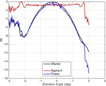
adding an empirically derived constant bias of 0.042◦to the elevation angle and re-computing X-factor, 587
the non-physical slope ofσ0was removed. Figure11shows the average return power,σ0and X-factor
588
after correction and averaging over a large area. We find that, post-correction,σ0remains flat over the
589
main lobe of the antenna, with no significant slope after the initial 0.042◦adjustment. 590
2.8. Radial Velocity Calibration
591
To achieve an error of 10 cm/s, one would require 7.7×10⁻⁴rad, or 4.4×10⁻²degree azimuth 592
angle accuracy, which is not achievable with the DopplerScatt encoder. Thus, it is necessary to calibrate 593
systematic errors in azimuth pointing during flight using the data themselves. In the past, some 594
researchers have used stationary land targets for calibration, but, in the presence of topography, the 595
accuracy of the look angleθis determined by knowledge of the topography, atmospheric delays, and 596
knowledge of the platform position. We do not have access to digital elevation models that meet the 597
accuracy requirements needed for calibration, and so must look for alternate approaches. We have 598
found that a novel approach that involving flying the same calibration lines over the ocean in opposite 599
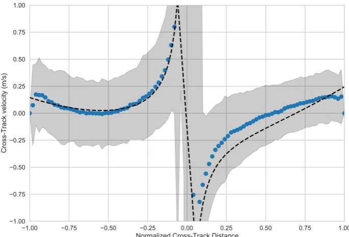
directions provides a feasible means for azimuth angle calibration. 600
The main challenge when using the ocean as a calibration target is the ocean Doppler induced by 601
surface currents. In the presence of a surface current and an azimuth bias, one has 602
vrS=−sin(α−αp)vpkδϕ+vWcos(α−αW) (41)
=−sin(α−αp)vpk
"
δϕ+vWx
vpk
#
+vWacos α−αp (42)
whereαpandαWare the azimuth directions of the platform and surface current, respectively;
603
vpk is the platform horizontal velocity divided by sinθ; and vWaandvWx are the surface current
604