Highlights in the hadron electromagnetic structure
EgleTomasi-Gustafsson1,,SimonePacetti2, andAndreaBianconi3
1IRFU, CEA, Université Paris-Saclay, 91191 Gif-sur-Yvette Cedex, France
2Dipartimento di Fisica e Geologia, and INFN Sezione di Perugia, 06123 Perugia, Italy 3Dipartimento di Ingegneria dell’Informazione, Università di Brescia and
Istituto Nazionale di Fisica Nucleare, via A. Bassi 6, 27100 Pavia, Italy
Abstract. In frame of a general view of proton electromagnetic form factors, two recent findings related to reanalyses of data are presented. Recent experiments in the scattering and in the annihilation region provided us with more precise data and/or extending the kinematical region, allowing a deeper analysis and a common view of these fundamental quantities. We will discuss two issues: the discrepancy between the form factors ex-tracted from unpolarized and polarizedepelastic scattering experiments, in connection with the commonly used dipole parametrization; peculiar oscillations ine+e− → pp¯ (γ) annihilation cross section, that become periodical when plotted as a function of the 3-momentum of the relative motion of the final proton and antiproton, after subtraction of a smooth function.
1 Introduction
Electromagnetic hadron form factors (FFs) are fundamental quantities that describe the internal struc-ture of non-pointlike particles, their charge and magnetic currents. Assuming that the interaction occurs through one photon exchange, FFs can be measured (through electron proton elastic scattering ande+e−↔pp¯ annihilations): in the first case, the transferred photon of virtual massQ2=−q2>0 is space-like, in the second case, the time-like photon has 4-momentum squaredq2>0. FFs are also di-rectly calculated, as they enter in the expression of the electromagnetic current: hadron models, after reproducing the static properties of hadrons, as masses and magnetic moments, should reproduce their dynamical content, parametrized by FFs. Schematically, FFs at large momentum transfer probe the quark structure of the hadrons whereas at low momentum transfer, they probe the size of the hadron.
The analytical properties of FFs justify a common interpretation of scattering and annihilation experiments. It is tempting to have a global definition of FFs, in the space and time-like regions. In [1] the definition of FFs was generalized as follows:
F(q2)=
Dd 4
xeiqμxμρ(x), qμxμ=
q0t−q·x, (1)
whereρ(x)=ρ(r,t) is the space-time distribution of the electric charge in a space-time volumeD.
e+p→ e+p as Fourier transform of a charge density:
F(q2)=δ(q0)F(Q2), Q2=−(q2
0− |q|2)>0, (2)
where the zero energy transfer is implied. In the annihilation channel:
F(q2)=
Ddte
i√q2t
d3rρ(r,t)=
Ddte
i√q2t
Q(t), (3)
whereQ(t) can be interpreted as the time evolution of the charge distribution in the domainD. In [1] a qualitative phenomenological picture of scattering and annihilation processes was presented, and the possibility of an observable dynamical polarization of the formed hadron pair was suggested.
Hadron FFs are investigated since decades, but recent findings and experimental possibilities have renewed interest in this field. High intensity electron beams, with large and stable polarization, to-gether with large acceptance spectrometers and detectors, and the development of hadron polarimetry allowed in particular to apply to the Akhiezer-Rekalo recoil proton polarization method [2, 3], that re-quires to measure the recoil proton(neutron) polarization in the scattering of longitudinally polarized electrons. These experiments, performed at MIT Bates (USA), MAMI (Germany) and JLab (USA) at large momentum transfer, brought very precise information on the ratio of the electric to magnetic FF for protons and neutrons and showed that this ratio is not constant, but decreases for increasing momentum transfer approaching zero at 9 GeV2. It was previously assumed that the electric and magnetic FFs follow a dipole dependence (Q2)−2. Still unpolarizedep scattering measurements seem to confirm such behavior. This discrepancy gave rise to a large number of theoretical papers and new experiments. We reanalyze the unpolarized cross section data in terms of FF ratio and show that the discrepancy between sets of data vanishes if one takes into account, besides effects of radiative corrections and parameter correlations, the effect of relative normalization.
The time-like region is accessible ate+e−colliders, as BABAR (USA), BESIII (China), and VEP-PII (Russia), through the reactione+e−→ pp¯ (γ) and at ¯ppcolliders as LEAR (CERN) and FermiLab (USA). In next future a high energy and high intensity antiprotons beam will be available at PANDA (FAIR, Germany). The presence of oscillating structures in the time-like FF data has been recently highlighted in [4, 5]. In particular the data present a regularity when plotted as a function of the rel-ative momentum of the outgoing hadrons. This pattern is tentrel-atively associated with the interference between two sources, respectively of the quark and of the hadron size, bringing the signature of the first instants of the hadron formation from the excited vacuum.
2 Reanalysis of Rosenbluth data
It has been assumed for long time that the proton electric FF, as well as the magnetic FFs of the proton and neutron, normalized to their magnetic moment, have aQ2-dipole dependence (Qis the four-momentum of the photon):
GD(Q2)=
1+Q 2[GeV]2
0.71
−2 ,
]
2[GeV
2Q
1 −10
1
10
D
σ
/
σ
0.8
0.9
1
1.1
1.2
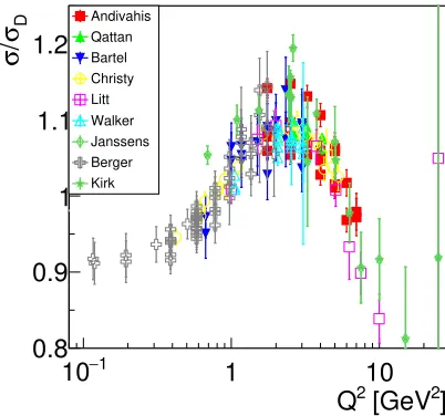
Andivahis Qattan Bartel Christy Litt Walker Janssens Berger KirkFigure 1.Cross section normalized to the dipole cross section,σ/σD, as a function of
Q2for different experiments.
dipole approximation corresponds to an exponential charge distribution. Moreover, from the QCD point of view, as elastic FFs represent the probability that a proton remains in its ground state after that each of its valence quarks has received a momentum squared,Q2, transferred by the virtual pho-ton. Scaling laws predict a (1/Q2)2dependence of the amplitude of the process [6, 7] (corresponding to two gluon exchange, the minimum number of exchanges needed for sharing the momentum among the three valence quarks).
However, several early experiments pointed out a deviation of the elasticep cross section from the (1/Q2)−5 behavior. Quoting a presentation of the data at the highest available transferred mo-menta, from Nobel prize R. Taylor: "There appears to be definite evidence in the data for a significant deviation from the dipole fit" [8]. The dipole normalized cross section
σ σD =
σexp red G2
D(/μ2+τ)
,
beingσexpred the measured reduced cross section, is reported in figure 1 as a function ofQ2, regardless of the value of. Hereτ=Q2/(4M2),M is the proton mass,μis the proton magnetic moment. The Q2 coordinates for the data at different are seen as vertically quasi-aligned symbols. Note that if these points form a cluster with overlapping error bars, it means that they are compatible with the relationGEGM/μGD. If points are not overlapping, then FFs do not follow a dipole behavior. In
general, and particularly at largeQ2, one can see that the dipole fit is not a good representation of the data. The deviation at largeQ2reaches 20-30% on the cross section and has to be attributed mainly to the magnetic term. The magnetic contribution to the elastic cross section becomes dominant at large Q2. Thereducedcross section of electron-proton elastic scatteringσ
red, in the one-photon exchange approximation, is linear in the variable=[1+2(1+τ) tan2(θ
e/2)]−1, beingθethe electron scattering
angle in the proton rest frame:
σred(θe,Q2)=
1+2E M sin
2(θ
e/2)
4E2sin4(θ
e/2)
α2cos2(θ
e/2) ×
(1+τ)dσ dΩ =G
2
E+τG2M, (4)
ff Q ff values of the FFs,G2
E andG2M, as the slope and the intercept (multiplied byτ), respectively, of this
linear distribution (Rosenbluth separation [9]).
The doubts on the deviation from the dipole approximation for the electric FF, became evident with the advent of polarization experiments. In the 70’s Akhiezer and Rekalo [2, 3] showed that the polarization of the scattered proton in the scattering of longitudinally polarized electrons on an un-polarized target (or the asymmetry with a transversely un-polarized target) contains an interference term proportional to the productGEGM. This observable would therefore be more sensitive to a small
electric contribution, and even to its sign (particularly important for the neutron case). A measure-ment of the ratio of the transverse to the longitudinal polarization of the recoil proton gives a direct measurement of the ratio of electric and magnetic FFs,R=GE/GM:
Pt
P =−2 cot(θe/2) M E+E
GE GM
, (5)
(E is the scattered electron energy) and it is free from systematic errors coming from the beam polarization and the analyzing powers of the polarimeter. The data based on the Akhiezer-Rekalo method, mostly taken by the JLab GEp collaboration ([10] and references therein), showed with unprecedented precision that the ratio of electric to magnetic FFs decreases asQ2increases. Below it is shown that recent reanalyses of Rosenbluth data in electron proton elastic scattering in terms of the FF ratio, show agreement between the value of this ratio whenever extracted from polarized or unpolarized experiments [11]. In particular the large sensitivity of the ratio to relative normalization of the cross section data solves the discrepancy, within the assumption of the one photon exchange mechanism.
2.1 Reanalysis of existing data
Problems of parameter correlations and limits inherent to the Rosenbluth have been discussed in [12]. Previous global analyses were done, discussing in particular the problem of normalization among dif-ferent sets of data, the omission of some of the data points [13] or reconsidering radiative corrections [14].
The following procedure to extract the FFs information from the unpolarized cross section has been suggested in [11]. Instead of extracting separatelyGE andGM, we write the reduced cross
section given in (4) as
σred =G2M(R2+τ), (6)
whereG2
M and R2 = (GE/GM)2 are considered as independent parameters. The unpolarized data
are fitted at fixedQ2. The procedure has the advantage to extract directly the ratio, by automatically accounting for the effect of the correlations betweenGEandGM. The parameterR2represents directly
the deviation of the linear dependence of the cross section from a constantvalue, whereas eventual general normalization and systematic errors are absorbed byG2
M.
If for some of the data values and errors consistent with the original publication are recovered, the data from [15] deserve a specific discussion. This work is especially representative, as it extends the individual FF extraction by the Rosenbluth method to the largest values ofQ2.
2.1.1 Data from [15]
]
2[GeV
2Q
0
1
2
3
4
5
6
7
8
9
Correction
0.94
0.96
0.98
1
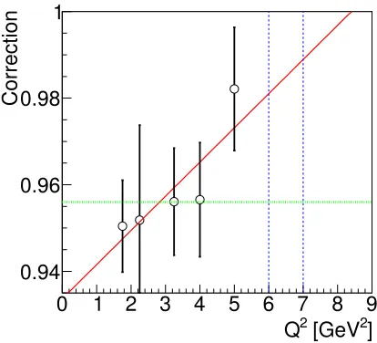
Figure 2.Correction factor as a function of
Q2. A linear fit (red line) shows an increasing of the factor. The dashed (blue) lines indicate that the extrapolated correction for the two HE points would be close to 1% instead than
5%, as applied in the original paper.
In the original paper the measured cross sections were published, warning that an uncertainty of ±5% affected the second setting, due to a poor knowledge of the acceptance of the spectrometer. This error, however, was not added to the tabulated error. Instead, it was taken into account as a constant relative correction, fixed on the two lowest valuesQ2 =1.75 and 2.50 GeV2(the cross section was measured at each setting for the lowestvalue). The cross section from the LE setting was larger by 4-5%. Assuming a lineardependence of the reduced cross section (that implies the dominance of the one-photon exchange mechanism), a fit of the HE data was done and the LE energy point was renormalized to lie on the straight line. Then, the same constant normalizationC =0.956, fixed on the lowQ2point, was applied to the cross section at allQ2(Analysis I). This procedure has the effect to enhance the slope, increasing the FF ratio. Note that forQ2 =6 and 7 GeV2only two points are present. The renormalization (lowering) of the first point changes essentially the slope of the linear fit.
The data were reanalyzed following several procedures. We recalculated the ratio using the data as published, without renormalizing the two settings and considering the LE points as additional, independent measurements. In this case the data points atQ2=1.75 and 2.5 GeV2are both included in the fit, constraining the fit to an average value (Analysis II).
We fit only the HE points (excluding therefore the two points atQ2 =6 and 7 GeV2). We find a slope consistent with analysis II, although affected by larger errors, as the number of points is smaller (Analysis III).
We repeat the normalization procedure, by aligning the LE point on the straight line fitting the HE points (Analysis IV). We note a systematic increase of the normalization factor (figure 2). Applying a normalization coefficient that is not constant withQ2but derived in order to align the LE point to the straight line defined by the HE points turns out to be equivalent to Analysis III in terms of slope and intercept.
]
2[GeV
2Q
0
2
4
6
8
10
2
)
M
/G
E
(G
2
μ
0
1
2
GEp
Andivahis
This work (Analysis II)
This work (Analysis III)
Figure 3.Color online.μ2
R2=μ2(
GE/GM)2 as a function ofQ2from (Andivahis: [15], green solid squares) as originally published; from Analysis II: without renormalization (red open circles); from Analysis III: omitting the lowestpoint (blue open squares) compared to the values from polarization experiments (GEp: [10], black solid circles).
section, by correcting the first point to be aligned. The results showed consistency with the hypothesis μ2R2 1 at largeQ2, as expected at that time. The tendency of the first two points to deviate from unity was operatively corrected by the renormalization procedure.
Among the available data, three sets [16–18] show a particular behavior, that is not consistent with the previous finding, giving a value of the ratio exceeding unity and growing withQ2.
For these experiments it was noted in [12] that radiative corrections and/or correlations are espe-cially large. The data from [18] were extracted detecting the proton instead of the electron. Besides the above mentioned corrections, at largeQ2 the contamination of the elastic peak by the inelastic e+p→e+p+π0reaction has to be carefully subtracted [10].
For [16, 17],G2
Mextracted from the present analysis is systematically lower, showing that these
measurements may be affected by a global systematic error probably due to normalization issues, whereas the results of [18] agree with the standard parametrization of the magnetic contribution.
Note that in [17] a somehow arbitrary renormalization was done by "changing the normalization of the small angle data from SLAC or DESY by±1.5% with respect to the large angle data (Bonn)". This normalization increased the FFs ratio towards unity.
3 Periodic oscillations in the time-like region
From the cross section, one extracts a generalized FF:
|Fp|2=
3βq2σ
2πα2
2+1τ
, (7)
(whereα=e2/(4π),β= √1−1/τ, τ= q2
4M2),Mis the proton mass.
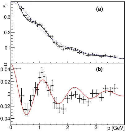
Plotting the generalized FF as a function of the 3-momentum of the relative motion of the final proton and antiproton, a systematic sinusoidal modulation appears in the near-threshold region, typical of an interference pattern, figure 4.
Through a Fourier analysis, the period is shown to correspond to a relative distance of 0.7-1.5 fm between the centers of the forming hadrons. It has been suggested that a rescattering process at the level of the newly formed hadrons interferes with the processes at a much smaller scale driven by the quark dynamics [4]. These oscillations may be interpreted as a signature of early mechanism of hadron creation.
We introduce a function of the form
F(p)=F0(p) + Fosc(p), (8)
wherep(q2)= √E2−M2,E =q2/(2M) − M, andpis the momentum of one of the two hadrons in the frame where the other one is at rest. The functionF0(p) is a smooth background, expressing the regular behavior of the FF over a longq2range, whereasF
osc(p) describes the overlapping oscillations.
The recent data are best reproduced by the functionF0proposed in [21]:
|F0(q2)| =
A (1+q2/m2
a)
1−q2[GeV]2/0.712
, A=7.7, m2
a =14.8 GeV2. (9)
The best fit function is then subtracted from the data, leaving a regular oscillatory behavior, figure 4. It has magnitude∼10 % of the regular term, and is well visible over the data uncertainties forp>3 GeV. We have fitted the difference between the BABAR data and the regular background termF0(p) with the four-parameter function
Fosc(p) = A e−Bp cos(C p+D). (10)
This difference is plotted in the lower panel of figure 4. The values of the parameters are, respectively, A =0.05±0.01,B= (0.7±0.2) GeV−1,C = (5.5±0.2) GeV−1, andD= 0.0±0.3. The relative errors in the parametersCandBshow that the oscillation period is better defined than the damping coefficiente−Bp. Two and a half oscillations are clearly visible over the reaction threshold, while for p>2.8 GeV the vertical error bars overcome the oscillation amplitudeA e−Bp.
The parameterDdefines the position of the first oscillation maximum that occurs atp=0 within the errorΔD P/(2π), where Pis the oscillation period. Estimating the oscillation periodP =1.13 GeV, the first oscillation maximum occurs atp=0 within an error of 0.05 GeV.
Sincepis a variable that is uniquely associated with the relative motion of the hadron, periodicity is associated to interactions (rescattering) between the forming hadrons after the virtual photon has been converted into quarks and antiquarks.
p
F
0.1 0.2 0.3
(a)
p [GeV]
0 1 2 3
D
0.04
−
0.02
−
0 0.02
0.04 (b)
Figure 4.a) FF data from BABAR as a function ofpLab, global fit: black solid line. b) after subtraction of a background function (blue dotted line), damped regular fit function (red solid line).
Distorted Wave Impulse Approximation (DWIA) formalism, following the scheme employed in [23]. The starting point is the Fourier transform
F0(p) =
d3reip·rM0(r), (11)
where we interpreteip·ras the plane wave final state of the ¯pppair in their center of mass, andM0(r)
as a matrix element describing the earlier stage of the process. Plane Wave Impulse Approximation (PWIA) corresponds to the absence of rescattering:ψf(r)=eip·r. In the distorted DWIA formalism a
simple factorized distortionD(r) is introduced:
ψf(r)=D(r)eip·r, (12)
whereD(r) is calculated as a Glauber-like eikonal factor:
D(x, y,z)=e−ib z∞ρ(x,y,z)dz, (13)
where ˆz// pandbis a complex number. Whenbis real, the rescattering potential is elastic, and it is attractive or repulsive (depending on the relative sign ofRe(b) andpz), whenbis pure imaginary,
the potential generates flux absorption or flux creation. The origin of an optical potential with an imaginary part is related, in general, to the fact that a multi-channel process is inclusively projected onto one channel alone.
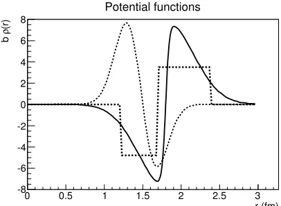
After testing several configurations, our best results have been obtained with double-layer imag-inary potentials, presenting twor-ranges where the potential phase is opposite,i.e.,they present an inner region where the ¯ppflux is produced and an outer region where the ¯ppflux is absorbed, as illustrated in figure 5. All of them are purely imaginary (Re(b)=0). The former two potentials have been calibrated to reproduce, as well as possible, BABAR data.
r (fm)
0 0.5 1 1.5 2 2.5 3
(r)
ρ
b
-8 -6 -4 -2 0 2 4 6 8
Potential functions
Figure 5.Three double-layer potentials used in (13) to calculate the final state distortion factorD(x, y,z). They may reproduce the FFs data (background and oscillations), with an opportune choice of the parameters.
atr ≈1-2 fm prevents most of the initial ¯ppchannel wave function from entering ther < 1 fm region. The "regeneration” effect due to the inner potential introduced above would have little effect on the total elastic and inelastic cross sections, since it affects only a very small component of the wave function.
On the other side, this small component which is nonzero at smallris essential for the coupling of the proton-antiproton pair with a virtual photon with virtualityq2 >4M2. The coupled regenera-tion/absorption mechanism produces, forr<2 fm, an alternance of regions where this component of the ¯ppwave function is enhanced or suppressed.
Specific conditions are necessary to reproduce the observed effect. An imaginary optical poten-tial that is mainly flux-generating in a region of small distances between the centers of the forming (and still overlapping) proton and antiproton, and mainly flux-absorbing at larger distances, produces systematic oscillations of the effective proton TL FF, consistent with the observed ones. At distances ≈1-2 fm this potential behaves as the optical potentials ordinarily used to reproduce ¯ppannihilation data: it damps the ¯ppflux by annihilating ¯pandpinto multi-meson states. A possible explanation for the regeneration features of the potential at smaller distances could be in terms of coupling between the ¯ppfinal channel and large-mass virtual states (like baryon-antibaryon) temporarily produced by the virtual photon. In order to reproduce the data, the transition from the generating to the flux-absorbing region must be sudden.
4 Conclusion
Form factors data in the space and time-like regions have been critically revised and reanalyzed. In the space-like region, the conclusion is that no real discrepancy exists between the FF extraction from polarized and unpolarized experiments, once all corrections (radiative, normalizations, correlations) are taken carefully into account. There is no need to claim for a large contribution of two-photon exchange. The presence of such contribution (beyond the expectedα−countingsize) would make the formalism ofepscattering experiments very involved, and invalidate most of the information of the nucleon structure extracted so far.
next future open the way to access the details of the hadron formation and of the inner composition of the hadron.
References
[1] E. Kuraev, E. Tomasi-Gustafsson, A. Dbeyssi, Phys. Lett. B712, 240 (2012) [2] A. Akhiezer, M. Rekalo, Sov.Phys.Dokl.13, 572 (1968)
[3] A. Akhiezer, M. Rekalo, Sov. J. Part. Nucl.4, 277 (1974)
[4] A. Bianconi, E. Tomasi-Gustafsson, Phys. Rev. Lett.114, 232301 (2015) [5] A. Bianconi, E. Tomasi-Gustafsson, Phys. Rev. C93, 035201 (2016) [6] V. Matveev, R. Muradian, A. Tavkhelidze, Lett. Nuovo Cim.7, 719 (1973) [7] S.J. Brodsky, G.R. Farrar, Phys. Rev. Lett.31, 1153 (1973)
[8] R.E. Taylor, Nucleon Form Factors above 6-GeV, in Proc. of the Int. Symp. on Electron and Photon Interactions at High Energies, SLAC, 1967 (Stanford Univ., SLAC, 1967) 78-101 [9] M. Rosenbluth, Phys. Rev.79, 615 (1950)
[10] A. Puckett, E. Brash, O. Gayou, M. Jones, L. Pentchev et al., Phys. Rev. C85, 045203 (2012) [11] S. Pacetti, E. Tomasi-Gustafsson, to appear in Phys. Rev. (2016).1604.02421
[12] E. Tomasi-Gustafsson, Phys. Part. Nucl. Lett.4, 281 (2007) [13] J. Arrington, Phys. Rev. C68, 034325 (2003)
[14] A.V. Gramolin, D.M. Nikolenko, Phys. Rev. C93, 055201 (2016) [15] L. Andivahis et al., Phys. Rev. D50, 5491 (1994)
[16] R. Walker et al., Phys. Rev. D49, 5671 (1994) [17] J. Litt et al., Physics Letters B31, 40 (1970) [18] I. Qattan et al., Phys. Rev. Lett.94, 142301 (2005)
[19] J. Lees et al. (BaBar Collaboration), Phys. Rev. D87, 092005 (2013) [20] J. Lees et al. (BaBar), Phys. Rev. D88, 072009 (2013)
[21] E. Tomasi-Gustafsson, M. Rekalo, Phys. Lett. B504, 291 (2001) [22] A. Bianconi, E. Tomasi-Gustafsson, Phys. Rev. C93, 035201 (2016) [23] A. Bianconi, M. Radici, Phys. Rev. C54, 3117 (1996)
![Figure 3. Color online. μ2R2 = μ2(GE/GM)2as a function of Q2 from (Andivahis: [15],green solid squares) as originally published;from Analysis II: without renormalization(red open circles); from Analysis III: omittingthe lowest ϵ point (blue open squares)compared to the values from polarizationexperiments (GEp: [10], black solid circles).](https://thumb-us.123doks.com/thumbv2/123dok_us/8147330.1358413/6.482.47.247.97.279/andivahis-originally-published-analysis-renormalization-analysis-omittingthe-polarizationexperiments.webp)