Nat. Hazards Earth Syst. Sci., 18, 2561–2602, 2018 https://doi.org/10.5194/nhess-18-2561-2018 © Author(s) 2018. This work is distributed under the Creative Commons Attribution 4.0 License.
Tree-based mesh-refinement GPU-accelerated tsunami
simulator for real-time operation
Marlon Arce Acuña1and Takayuki Aoki2
1Department of Nuclear Engineering, Tokyo Institute of Technology, 2-12-1-i7-3, Ookayama, Meguro, Tokyo, Japan 2Global Scientific Information and Computing Center, Tokyo Institute of Technology,
2-12-1-i7-3, Ookayama, Meguro, Tokyo, Japan
Correspondence:Marlon Arce Acuña ([email protected]) Received: 20 October 2017 – Discussion started: 10 November 2017
Revised: 16 July 2018 – Accepted: 13 August 2018 – Published: 21 September 2018
Abstract. This paper presents a fast and accurate tsunami real-time operational model to compute across ocean-wide simulations completely on GPU (graphics processing unit). The spherical shallow water equations are solved using the method of characteristics and upwind cubic interpolation to provide high accuracy and stability. A customized, user inter-active, tree-based mesh-refinement method is implemented based on distance from the coast and focal areas to gen-erate a memory-efficient domain with resolutions of up to 50 m. Three specialized and optimized GPU kernels (Wet, Wall and Inundation) are developed to compute the domain block mesh. Multi-GPU is used to further speed up the com-putation, and a weighted Hilbert space-filling curve is used to produce a balanced workload. Hindcasting of the 2004 In-donesian tsunami is presented to validate and compare the agreement of the arrival times and main peaks at several gauges. Inundation maps are also produced for Kamala and Hambantota to validate the accuracy of our model. Test runs on three Tesla P100 cards on Tsubame 3.0 could fully simu-late 10 h in just under 10 min wall-clock time.
1 Introduction
The turn of the 21st century showed us, as never before, the reality of the terrible and devastating damage and death that tsunamis can cause. In 2004, a massive earthquake off Sumatra Island of magnitudeMw=9.0 on the Richter scale triggered a tsunami with deadly consequences. According to the World Health Organization, the death toll for these events exceeds 200 000 (WHO, 2014) in several countries
spread along the Indian Ocean. Not much later in 2011, a tsunami triggered by aMw=9.0 earthquake on the east coast of Japan in the Tohoku region produced yet another disaster. Over 15 000 people died from these events, with massive destruction of port and city infrastructure, housing, and telecommunications. Additionally, the subsequent nu-clear crisis was due to the tsunami-induced damage of several reactors in the Fukushima nuclear power plant (Motoki and Toshihiro, 2012).
It was original because it introduced a function to add points in the shoreline to improve tracking. Recently, MOST has been ported for GPU computing (Vazhenin et al., 2013). A more recent model is GeoClaw, which implements a unique approach to deal with the issue of transferring fluid kinemat-ics throughout nested grids by refining specified cells during simulation to improve resolution in those areas (Berger and LeVeque, 1998). More recent models incorporate a real-time application such as RIFT (Real-Time Inundation Forecast-ing of Tsunamis) (Wang et al., 2012). Like several of the previous models, a leapfrog scheme is also used for these real-time models, and a linear SWE is solved in certain ar-eas for lighter computation. COMCOT (Cornell Multi-grid Coupled Tsunami Model) from Cornell University is another example using this approach (Liu, 1998). EasyWave is an-other model (Babeyko, 2017) which employs linear approx-imations to improve speed and employs a leapfrog scheme as its numerical scheme. The latest version of EasyWave in-troduced GPU to accelerate parts of the existing CPU code. More recently, GPU-based models have been developed, like NAMI DANCE (Zaytsev et al., 2006) in its latest version. Additionally, a better known GPU model, Tsunami-HySEA (Macías et al., 2017), has been extensively tested and is cur-rently used by the Centro di Allerta Tsunami (CAT) in Italy. In order to include the effect of pressure, since the 1990s, some models have taken the direction of solving non-hydrostatic models using the depth-integrated Boussinesq equations (BEs) instead of the SWEs for tsunami propa-gation. Initial efforts considered them to be weak nonlin-ear models (Peregrine, 1967); however, models for nonlinnonlin-ear equations were also developed not long after (for instance, Nwogu, 1993; Lynett et al., 2002). Solving the Boussinesq equation is, in general, more computationally demanding than solving the SWEs and in order to reduce the computa-tional time, some techniques have been implemented, such as using parallel clusters or introducing nested grids. An exam-ple of this is FUNWAVE-TVD (Shi et al., 2012), which is an extended version of FUNWAVE, a run-up and propagation model based on fully nonlinear and dispersive Boussinesq equations (Wei et al., 1995). FUNWAVE introduced a nested-grid method, and its later version was fully parallelized us-ing MPI-FORTRAN. A well-known non-hydrostatic model which also implements two-way grid nesting is NEOWAVE (Non-hydrostatic Evolution of Ocean WAVE; Yamazaki et al., 2011). Another one of these models is BOSZ (Roeber and Cheung, 2012), which combines the dispersive effect from the BEs with the shock-capturing ability of the non-linear SWEs. BOSZ is mainly used for nearshore simulation, since it is based on Cartesian coordinates and not suited for large areas. Additionally, it does not implement nested grids. Recently, efforts to solve the modeling equations in three dimensions have been made as well. Although these mod-els tend to capture difficult coastlines very well and can in-clude multiple fluids or even materials, the computation cost is still so great that it makes it only possible to apply them
effectively in small areas and it is not viable for transoceanic propagations. Some examples are SELFEs (semi-implicit Eulerian–Lagrangian finite elements; Zhang and Baptista, 2008; Abadie et al., 2010, 2012; Horrillo et al., 2013).
In this work, we present a new approach for a tsunami op-erational model that retains a high degree of the complexities of the physics involved and delivers a fast and accurate sim-ulation. This speed also enables real-time operation: a user can start forecasting simultaneously as a tsunami event oc-curs. Results are generated faster than real time. The main goal is to accomplish a wide-area, ocean-size computation in short time while using resources efficiently. Our model, referred to hereinafter as TRITON-G (Tsunami Refinement and Inundation Real-Time Operational Numerical Model for GPU), implements a full-GPU computing approach for the whole tsunami model, composed of generation, propagation and inundation. Specialized kernels are developed for each part of the tsunami computation, and multi-GPU is used for further acceleration. Load balance is obtained using a weighted Hilbert space-filling curve. TRITON-G solves the nonlinear spherical shallow water equations across the en-tire domain to preserve the complexity of the propagation and the effects near the coastline. The method of character-istics with directional splitting and a third-order interpola-tion semi-Lagrangian numerical scheme is used to solve the governing equations. This allows for high accuracy and min-imizes effects of numerical dispersion and diffusion while also giving the ability to choose a larger time step compared to using a Runge–Kutta scheme and at the same time per-mits a light stencil suitable for fast computation. We imple-ment a tree-based block refineimple-ment to generate a computa-tional mesh that is flexible, light and can track complex coast-lines. Customized refinements by distance and focal area were developed, which permitting an efficient use of mem-ory and computational resources. In a collaborative project with RIMES (Regional Integrated Multi-Hazard Early Warn-ing System, 2017), we utilize their existWarn-ing databases for bathymetry and fault sources where available and success-fully deployed TRITON-G as their tsunami forecast opera-tional model.
M. Arce Acuña and T. Aoki: Tree-based mesh-refinement GPU-accelerated tsunami simulator 2563 2 Governing equations
The spherical nonlinear shallow water equations (SSWEs) are used to compute the tsunami propagation. In small, spe-cific areas where inundation needs to be computed, the Carte-sian coordinate version of the SWEs are solved instead (see Toro 2010). The SSWE (Williamson et al., 1992; Swarz-trauber et al., 1997) can be written as
∂h ∂t +
1 acosθ
∂ ∂λ(hu)+
1 a
∂ ∂θ(hv)−
hv
a tanθ=0, ∂hu
∂t + 1 acosθ
∂
∂λ
hu2+g 2h
2+1 a
∂huv
∂θ − hv
a tanθ −f +u
atanθ
hv+ gh acosθ
∂z
∂λ+τλ=0, ∂hv
∂t + 1 acosθ
∂hvu ∂λ + 1 a ∂ ∂θ hv2+g
2h
2−hv2 a tanθ +f+u
atanθ
hu+gh a
∂z
∂θ+τθ=0, (1)
whereλstands for the longitude coordinate,θfor the latitude coordinate,his the water depth,huandhvare the momen-tum in longitude and latitude, respectively, with correspond-ing velocitiesuandv,gis gravity,ais the radius of the Earth, zis the bathymetry (submarine topography),fis the Coriolis force defined asf=2sinθ withbeing the rotation rate of the Earth and τ is the bottom friction term. The bottom friction is determined using the Manning formula:
τλ=
gn2 h7/3hu
p
(hu)2+(hv)2, τθ=
gn2 h7/3hv
p
(hu)2+(hv)2, (2)
where n is the Manning’s roughness coefficient. The de-fault value used for n is 0.025 across all domains except for specific areas where more detailed values in the coast-line are given in a database. The parameters used in this work area=6.37122×10⁶[m],=7.292×10⁻⁵[s−1] and g=9.81 [m s−2].
3 Numerical methods and boundary conditions 3.1 Methods of characteristics for SSWEs
The SSWEs are solved using the method of characteris-tics (MOC). A method developed in the 1960s, explained in detail by Rusanov (1963). MOC is applied to reduce hyper-bolic partial differential equations, such as the SSWEs, to a family of ordinary differential equations. A traditional ap-proach when using MOC is to introduce a dimensional split-ting (Nakamura et al., 2001) in the 2-dimensional equations to create a smaller stencil and lighter computation. A numer-ical scheme is regarded as well-balanced, or satisfying the C-property (Bermúdez and Vázquez, 1994) if it preserves
steady states at rest, for instance, the undisturbed surface of lake. When the fluid is at rest, i.e.,u(x, t )=0 then the constant water heightHdefined asH (x, t )=h(x, t )+z(x) represents a steady state that should hold in time and not pro-duce spurious oscillations (LeVeque, 1998). In order to make the model well-balanced, the SSWEs are solved forH dur-ing the simulation to guarantee this steady state. The origi-nal variablehis simply obtained back from the expression h=H−z.
In order to apply the method of characteristics, first the SSWEs Eq. (1) are rewritten in vector form as
∂U ∂t +A
∂U ∂λ +B
∂U
∂θ +S=0 (3)
with U= h hu hv
A= 1
acosθ
0 1 0
02−u2 2u 0 −uv v u
B=1 a
0 0 1
−uv v u
02−v2 0 2v S=
−hvtanθ a −f+u
atanθ
hv−huv a tanθ+
gh acosθ
∂z ∂λ
f+u atanθ
hu−hv 2 a tanθ+
gh a ∂z ∂θ ,
where0≡√gh. Using the directional splitting technique on Eq. (1), three equations are produced: an equation for each coordinate (longitude λand latitude θ) and a third for the source termS. The latter equation simply represents an or-dinary partial differential equation for the source term while, Eqs. (4) and (10) for the coordinates are in advection form. These last two equations are written in diagonal form in or-der to find the Riemann invariants and characteristics curves; a detailed description of this procedure can be found in Ogata and Takashi (2004) or Stoker (1992). The equation for the longitude coordinateλgiven by
∂U ∂t +A
∂U
∂λ =0 (4)
has eigenvalues3given by
3λ±= 1
acosθ(u+0), 3
λ
3= 1
acosθu, (5)
which inserted in the diagonal form of Eq. (4) leads to D±
Dt
0±u 2
whereD/Dtrepresents the material derivative. Equation (6) means that the solution at a given grid pointiis determined from two characteristic curves along C+ andC− (Fig. 1). The result at a timen+1 can be found by adding and sub-tracting the expressions in Eq. (6) respectively to obtain 0in+1=1
2
0++0−+1 2 u
+− u−
(7)
uni+1=1 2
u++u−+2 0++0− , (8)
where 0± andu± are the values at a timen, at positions which might not necessarily lie on a grid point. An interpo-lation is applied in order to determine these values, and with them solve Eqs. (7) and (8).
Following a similar procedure as Yabe and Aoki (1991), Yabe et al. (2001) and Utsumi et al. (1997), we utilize a cubic-polynomial approximation on the grid profile to find the interpolated values. The polynomial is defined as
F (λ)=aλ3+bλ2+cλ+d (9)
with
u1t >0
a=fi+1−3fi+3fi−1−fi−2 61λ3
b=fi+1−2fi+fi−1 21λ2
c=2fi+1+3fi−6fi−1+fi−2 61λ
d=fi
u1t ≤0
a=fi+2−3fi+1+3fi−fi−1 61λ3
b=fi+1−2fi+fi−1 21λ2
c=−fi+2+6fi+1−3fi−2fi−1 61λ
d=fi
.
A similar analysis can be made for the latitude equationθ ob-tained from the splitting method, given by
∂U ∂t +B
∂U
∂θ =0 (10)
with analogous results for the eigenvalues and curves 3θ±=
1
a(v+0), 3
θ
3= 1
av, (11)
D± Dt
0±v
2
=0. (12)
From which similar expressions as Eqs. (7) and (8) can be found in order to estimate the values forhandhv.
The equations for the coordinates are solved using the fractional step method. Following this method, the source term given by
∂U
∂t +S=0 (13)
Figure 1. Space–time diagram showing the characteristic curves C± where black points represent the grid points, white points represent the values0±andu±at timento be interpolated to find0n+1andun+1.
is added to the solution obtained for Eqs. (4) and (10) . For the source term, central finite differences are used to solve the bathymetry term while the remaining values (cosine, tangent terms) can be solved analytically at each grid point since the variables are known straightforwardly.
In order to validate the implementation of the numerical methods for the SSWEs, we used the benchmark described in Kirby et al. (2013), where an initial Gaussian wave is prop-agated on an idealized sphere with water depthh=3000 m. Results after 5000 s show good agreement with the results re-ported which confirms the accurate propagation of the wave on the sphere and the effects of the curvature and Coriolis force.
3.2 Run-up calculation
The Cartesian SWEs are solved in specific areas of just a few kilometers where inundation has to be calculated. For this case we use a finite volume implementation (Bradford, 2002; LeVeque and George, 2014) briefly described here. The sur-face gradient method (SGM) (Zhou et al., 2001) is utilized to solve the SWEs. This method uses the data at cell centers to determine the fluxes. In general, depth gradient methods cannot accurately determine the water depth value at cell in-terface, since effects of the bed slope or small variations in the free surface cannot be determined accurately. These in-accuracies are spread during the computation, resulting in an incorrect simulation of the inundation. In order to overcome this, the SGM uses a constant water levelH. Figure 2 de-picts the stencil for the water-depth reconstruction. By using the constantH as the total water depth at the cell interface (i+0.5) instead, the water depth be can determined accu-rately. In order to reconstruct the water depth, the following expression is used:
hL,Ri+0.5=max HL,Ri+0.5−zi+0.5,0, (14) wherezis given by
zi+0.5=(zi+zi+1)
M. Arce Acuña and T. Aoki: Tree-based mesh-refinement GPU-accelerated tsunami simulator 2565
Figure 2.Reconstructed water depthhL,Rfor inundation (LeVeque and George, 2014).
A MUSCL scheme (Yamamoto and Daiguji, 1993) is used to find the flux value, while local Lax–Friedrichs (LeVeque, 2002) is used to solve the bed slope source term. For the time integration, a third-order TVD Runge–Kutta scheme was used. This method is nonconservative; however, in tests the difference on mass conservation has shown to be al-most negligible. Lastly, the bottom friction is computed using Manning’s formula.
This run-up implementation assumes a thin film of water on land defined asε. This parameter, set much smaller com-pared to the wave height, allows the computation of the wave inundation over land while keeping it stable. If the water height is less thanε(i.e.,h < ε) then the height value is fixed as εand the momentum is set as rest (i.e., hu=hv=0) on that grid point. This implementation has proven to be robust and stable under different benchmarks and simulations (Vin-cent et al., 2001). This numerical-method implementation to-gether with a slope limiter produces a monotone scheme that preserves water positivity.
The one-dimensional dam break benchmark (Stoker, 1992) was used to compare the results with its analytical so-lution and good agreement was found. The shock wave was successfully captured for different initial water heights.
The parabolic bowl problem proposed by Thacker (1981) was also used to compare the accuracy of the inundation. The bottom bathymetry is given by
z(r)= −D0
1− r 2 L2
, (16)
while the water height at a timetcan be found from the ana-lytical solution
H (r, t )=D0
1−A2 1 2 1−Acosωt −1−
r2 L2
1−A2 (1−Acosωt )
r=(x−Lx/2)2+ y−Ly/22
ω=
q
8gD0/L2
A=(D0+η) 2−D2
0 (D0+η)2+D02
. (17)
We use these parametersLx=Ly=8000,L=2500,D0= 1 andη=0.5. Two grid sizes were used for testing, 80×80 and 160×160 cells. Figure 3 shows the oscillating water in the bowl at different times. As it can be seen, the inundation method is able to capture the analytical solution of the water height well as it evolves in time on the different grid sizes. Measurements on this tests showed a third-order reduction of the error as the valueεwas decreased.
3.3 Tsunami source model
TRITON-G focuses on propagation and inundation while re-lying on external parameters for the generation stage. In or-der to start a simulation, the initial condition is provided directly by RIMES using their preferred fault theory and model. In the generation process, a good initial source model is essential in order to obtain an accurate simulation. How-ever, due to the complex nature of the source dynamics dur-ing an earthquake and the difficulty to track it in real time (as it happens), it is currently beyond our grasp to obtain these parameters precisely and instantly. For these reasons we opted for a coseismic deformation. This deformation is calculated from the theory of displacement fields proposed by Smylie and Mansinha (1971). Their objective was to pro-vide a closed analytical expression that “facilitates the inter-pretation of near-fault measurements”. The expressions pro-vided, valid at depth and surface, consist solely on algebraic and trigonometric functions that can be readily evaluated nu-merically based on a few source parameters like dip, strike, slip and length. These values are obtained from RIMES’ databases online or loaded from a file. The original source generation code, provided by RIMES, was written for CPU and ported by us to GPU for this study.
3.4 Boundary conditions
Two kind of boundary conditions are used: open and closed. Open boundary set conditions to allow waves from within the model to leave the domain through an edge without affecting the interior solution. Closed boundaries, which keep the fluid inbound in the domain, physically prevent water flow across the edges. A wall boundary condition creates a total physical reflection when a wave hits a dry point.
In Eq. (1) the term cosθ in the denominators produces a singularity at the poles of the spherical coordinate sys-tem. When working on a complete sphere, special techniques and treatments are required to compute values over the poles without divergence. In this study, the domain chosen repre-sents a portion of the Earth centered in the Indian Ocean and does not extend near the poles in any circumstance which permits us to avoid this pole singularity.
Figure 3.Parabolic bowl problem cross section with=10−4on(a). Water depth error for parabolic bowl problem on(b).
closed boundary condition at the north and west edges. All coastlines have wall boundary conditions except for the spe-cial cases where particular regions set asinundationare de-fined. In those cases a complete run-up is computed using the methods described in previous sections. Since the inun-dation method is relatively computationally intensive, using two kinds of boundaries for the coasts permits us to focus computational resources just in areas of interest.
The boundary between spherical and Cartesian coordi-nates that occur in specific areas where inundation is com-puted has no special treatment since the area covering the inundation consists, by design, of just a few kilometers (Fig. 5a). This makes the difference between meshes almost negligible and does not noticeably affect the result.
4 Tree-based mesh refinement and bathymetry
An efficient use of resources, memory and computation re-quires a mesh that covers areas of interest with high reso-lution only where desired but leaves the rest of the domain coarser. The concept of this approach is similar to that of the adaptive mesh refinement, initially introduced by Berger and Oliger (1984) and Berger and Colella (1989) in the 1980s as a method to solve partial differential equations (PDEs) on an automatically changing hierarchal grid, solving for a set accuracy on certain areas of the interest instead of unneces-sarily overly refining the entire domain.
To generate the mesh for the domain, we use a customized tree-based mesh refinement without the need of remeshing during simulation since the geometrical features remain un-changed. We briefly explain the process of tree-based refine-ment (Yerry and Shephard, 1991). Figure 4 illustrates this procedure using a moon-shaped green point as the area of interest. At each level, the domain and its tree structure, called quadtree, is presented. Initially just a quadrant and its quadtree root exist. Each quadrant represents a block of
Figure 4.Tree-Based block refinement with quadtree structure and Hilbert space-filling curve for five levels.
M. Arce Acuña and T. Aoki: Tree-based mesh-refinement GPU-accelerated tsunami simulator 2567
around the points of interest while the quadtree data structure associated with it keeps track of the blocks’ connectivity.
The difference in spatial resolution between two adjacent levels is called the refinement ratio. For nested grids, this ratio is any positive integer. However using large integers tends to introduce inaccuracies in the computation. The ex-istence of an abrupt change from one level to the next re-quires a special boundary treatment, especially when com-plex bathymetry or topography is involved. For tree-based refinement, this ratio is fixed as1xl/1xl+1=2, wherel rep-resents the block level and1xthe grid resolution. This con-stant and small ratio creates a smooth wave transition be-tween levels.
4.1 Customized mesh generation
The domain used for this work represents a large portion of the Indian Ocean (Fig. 5), which initially consists of a uniform mesh of 56×30 blocks, each made up of 65×65 node-centered cells. Using the tree-based refinement, cialized customizations are developed to adapt it to our spe-cific needs. In general, mesh-refinement methods utilize an error estimation as the rule to determine if a block should be refined; however, in this implementation the refinement de-pends on a target grid resolution combined with two factors: the block’s distance from the coastline and the presence of a focal area.
Since the refinement rule’s first factor depends on the dis-tance of the block to the shoreline, the objective is to recur-sively refine blocks close to the coast until reaching a tar-get high-resolution threshold, while blocks far in the ocean remain with a coarser resolution. This process involves two steps: determining the block’s distance from the coast and checking if its distance is within refinement.
Accurately estimating the geo-distance between two points can be a complex task since the surface of the Earth is not a perfect sphere. However, for our refining purposes, a rough estimate is enough to determine the distances between the shoreline and the blocks. This is achieved by creating a signed distance function based on the level-set method. A de-tailed explanation of this procedure can be found in Fedkiw and Osher (2003). The distance function’s zero level is repre-sented by the cells along the shoreline (z=0). Positive dis-tances represent cells on land while negative disdis-tances rep-resent cells on the ocean. Using these distance values, each block is tested for refinement. Blocks with one cell or more within a certain distance from the coast, called refinement stripes, are flagged for refinement until they reach the fine-target resolution. The width of the refinement stripe is prob-lem dependent and is input by the user based on their needs. For this study the initial resolution at ground level 1 is 2 arcmin (an arcminute being 1/60 of a degree, at Earth’s equator equivalent to 1852 m) and the target finest resolution is 0.03125 arcmin (approximately 50 m), generating a total of seven levels. This block refinement process can accurately
trace complex coastlines and focus high resolution only in the shores. A downside is the considerably large number of total blocks generated, over 230 000 in initial tests, which represents over 100 GB of memory storage.
In order to reduce the memory footprint, we used the fact that only certain regions need high resolution, which inspired us to use a second refinement factor namedfocal areas(FAs). This second factor is an additional constraint which consists of locating a convex polygonal area on the domain, which serves as a refinement delimiter. It is possible to locate more than one at a time, and since this is an additional constraint to the first refinement step, only blocks flagged for refine-ment at the first step need to be tested again. On this sec-ond test, a block is tested if it is inside or outside a focal area. If a block is completely outside the focal area, then it is unflagged for refinement. Only blocks partially or to-tally inside the focal area are refined. The process of deter-mining if a block lies inside or outside a focal area is based on collision detection theory using the separating axis theo-rem (SAT). This is a well-known theotheo-rem applied to physical simulations (Szauer, 2017) and consists of a relatively light algorithm for 2-D, which allows us to test large number of blocks rapidly. A description of the SAT can be consulted in Moller et al. (1999) or Gottschalk et al. (1996). Since the fo-cal area is an additional constraint, it can be toggled active after any chosen level. A specific number of levels can be re-fined without this constraint while the following are affected and delimited. Additionally, all dry blocks at Level 7 (high-est resolution) that are inside a FA are considered inundation areas. This implies that run-up is computed on the coastlines instead of using a reflective boundary.
The last step in the mesh generation consists of the re-moval ofland dry-blocks. Considering that tsunami inunda-tions, with few excepinunda-tions, generally extend tens to hundreds of meters inland, it becomes clear that blocks located deep in-land are unnecessary for the computation. For this reason all blocks whose cells’ distances are larger than a land–distance threshold are considered land dry-blocks and deleted from the domain.
gener-Figure 5. (b)Mesh refinement for Indian Ocean domain with four focal areas (FAs): Mozambique, Comoros, Seychelles and Sri Lanka. (a)Zoom on the Seychelles (right panel) and Sri Lanka (left panel) regions. FAs are highlighted in green.
ated by TRITON-G can be either computed in real time or loaded from a repository at the beginning of the simulation. 4.2 Halo exchange
Blocks must exchange results with their neighbors after each time step for the next iteration. For this purpose they share a boundary layer in their adjoining sides. This layer, or halo, extends over the neighbor’s grid and updates in one of three kinds of operations: copying, coarsening or interpolating.
If two neighbor blocks have the same level, then the halo is readily updated by exchanging values directly without any further computation; this represents a copying swap. If the neighbors are at different levels (landl+1) then additional computation is required before the halo exchange. If the block’s neighbor is one level up, then values for the halo are
averaged down from the block with higher accuracy before swapping. This has a cascade effect of passing down better accuracy to blocks with lower resolution. The last case, in-terpolating, occurs when the block’s neighbor is one level down. For this, the values for the halo are interpolated from the neighbor block using a third-order polynomial interpo-lation, similarly as in Eq. (9). The portion of the boundary stencil used for interpolation is shown in Fig. 6.
The new values for the halo for the north (N) and east (E) edges can be found from
fPN1,E=1
4 fj+4fj+1−fj+2
fPN2,E=1
4 −fj+6fj+1−fj+2
M. Arce Acuña and T. Aoki: Tree-based mesh-refinement GPU-accelerated tsunami simulator 2569
Figure 6.Halo interpolation stencil for the four edges:(a)west, south and(b)east, north.
since they are analogous orientations. For the south (S) and west (W) edges, similar expressions are used
fPS,1W=1
4 −fj−2+4fj+1+fj
,
fPS,2W=1
4 −fj+6fj+1−fj+2
. (19)
In order to avoid spurious waves that might be generated from interpolating the water height value h, constant water levelHis used instead, and the original variable is recovered by using the relationh=H−z.
4.3 Topography and bathymetry
The data used in this study for bathymetry and topogra-phy comes from different sources. Initially, The General Bathymetric Chart of the Oceans (Oceans (GEBCO), 2017) database is used on the entire domain. GEBCO is freely available in 30 arcsec spatial resolution. When coarser reso-lution is needed, values are averaged from this database. On the contrary, if finer resolution is needed, a third-order inter-polation is implemented to generate the new values. Where available, databases with more precise measurements are used to replace the original GEBCO database. For the focal areas in Mozambique, Comoros, Seychelles and Sri Lanka, RIMES’ proprietary databases generated from field measure-ments were provided to us to estimate the inundation more accurately.
5 GPU computing
The introduction of C-language extension CUDA (NVIDIA, 2017a) by NVIDIA® represented a disruption in the tradi-tional way simulations were done. The availability to pro-gram general purpose GPU cards permitted researchers to no longer exclusively perform calculations on CPU. Due to the intrinsic parallelism of graphics, GPUs evolved to de-liver hundreds and thousands of processors more in a card than CPUs. The main reason behind the exceptional
perfor-mance of GPUs lies in the specialized design for compute-intensive, highly parallel computation, with transistors ded-icated exclusively to processing as opposed to flow control and data caching. The latest NVIDIA Tesla cards P100, with Pascal architecture, have a peak performance of 9.3 Teraflops on single precision and 4.7 Teraflops on double precision (NVIDIA, 2017b). We take advantage of this technology to develop a full-GPU implementation to deliver fast forecast-ing results.
5.1 SSWE GPU kernels
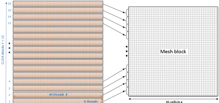
CUDA provides kernels as a way to define functions that are executed in parallel on GPU. Each kernel launch is organized in a grid of blocks of CUDA threads. The clear analogy be-tween CUDA blocks and mesh blocks provided a guide to organize the grid for GPU execution. The SSWEs are com-puted exclusively on GPU by processing the mesh blocks created during the domain refinement step and are stored in a structure of arrays on GPU global memory. Each mesh block has a size of(65+4)×(65+4), where the “4” corresponds to the total size of the halo. CUDA threads can be organized in any three-dimensional block configuration as needed for the problem. Since GPUs process threads in warps of 32, using multiples of this number is desirable to avoid performance penalties.
difference occurs in the case of a dry block; in this case, cells that represent land or coastline compute a reflective wall boundary.
To process all the mesh blocks, this two-dimensional CUDA block configuration is extended along thezdirection as many times as mesh blocks exist. The computation of the 65th cells is done separately with a specialized kernel based on the SSWE kernel.
In the case of Cartesian SWE kernel, the grid chosen for this kernel is different than that of the kernel for SSWE. In this case, a mesh block is subdivided and covered by CUDA blocks of 16×16 threads. The excess of threads at the edges is not computed using a conditional limiting the grid size.
The source fault code was ported to GPU from the original C version. Due to the exclusively arithmetic operations and lack of a stencil memory access involved, a 20t imes speed up was achieved, reducing the computation of the initial con-dition to just a few seconds.
Several kernel optimizations were applied in order to ac-celerate the model’s time to solution. This includes using the latest CUDA version to take advantage of the latest com-piler updates. To avoid branch divergence as much as possi-ble parts of the numerical method were rewritten to eliminate conditionals. Precomputing terms that do not change in time like trigonometric terms depending on the longitudeθ, stor-ing them on arrays and reusstor-ing them durstor-ing the simulation. Using built-in functions to compute complicated exponen-tials like those in the Manning formula. Although the opti-mizations provided speed up, no sacrifice was incurred on precision. All GPU computations are performed on double precision.
5.1.1 Halo update on GPU
Update of the halo region of each mesh block after each time step with the latest values from neighbor blocks represents three different kinds of exchanges: copying, coarsening or in-terpolating. These operations are performed entirely on GPU. Kernels designed for each kind of exchange were created. In order to efficiently process the block edges, three lists are generated containing the list of halos that require each op-eration. This way the kernels can be launched concurrently, and each focus on a different task minimizing the need for conditional divergences.
5.1.2 Specialized kernel types
By analyzing the domain’s bathymetry, it is easy to notice that some mesh blocks contain only wet points while others are a combination of dry and wet points. This idea is used to replicate the SSWE kernel in two variations.
The first SSWE kernel, namedWet, is used to compute the free propagation of the wave on wet-only blocks. The second SSWE kernel, namedDry, is used to compute the wave prop-agation with coastline boundaries in wet–dry mixed blocks.
The main difference in the code between them is the addi-tional treatment for the wall boundaries at coastlines in the case of the Dry kernel. A third kind of kernel (Inundation), specializes in computing the run-up on dry blocks inside fo-cal areas.
The result of the kernel assignment is illustrated in Fig. 8, where blocks flagged as wet are shaded in red, dry blocks are shaded in green and inundation blocks in blue. As ex-pected dry blocks tend to extend where coastlines lie while wet blocks are spread out in the open ocean. When inside a focal area, dry-type blocks at level 7 are reflagged as inun-dation type. An example of this can be seen in the left image of Fig. 8 for the Sri Lanka FA, with inundation blocks in blue. Whereas a single kernel would be too complicated and inefficient to compute the entire domain, splitting down the computation in specialized kernels for each type of block not only provides a simpler way to process the blocks through lists, but also gives the ability to fine tune them independently for higher performance.
5.2 Space-filling curve and multi-GPU
In order to implement multi-GPU for further acceleration, first an appropriate domain partition must be chosen to guar-antee an even workload among cards. Since a uniform mesh is not being used, this partition is nontrivial. Although block connectivity is kept using a quadtree structure, this does not provide information about the blocks ordering. For this pur-pose we use the space-filling curve (SFC) (Sagan, 1994) as a way to trace the blocks’ ordering on the domain.
SFC is a curve that fills up multi-dimensional spaces and maps them into one dimension. It has many properties de-sirable for domain partition; it is self-similar and it visits all blocks exactly once. We use the Hilbert curve in this work since it tends to preserve locality, which keeps neighbors to-gether and does not produce large jumps in the linearization like other curves tend to, such as the Morton curve. Figure 4 shows the Hilbert curve generation as a red line overlying the quadrants. It starts as a bracket on the first four quadrants, and with each spatial refinement, the bracket gets replicated subject to rotations and reflections to guarantee the charac-teristic of the curve. The result of generating a Hilbert SFC for the Indian Ocean domain is shown in Fig. 9. By using this curve as a reference, it is possible to establish the block ordering to partition the domain on even portions. The result of splitting the domain for eight GPUs is shown in Fig. 10, where each portion is represented by a different color. In this case, seven GPUs have a total of 981 blocks each, and the eighth GPU has a total of 982 blocks, making it a well-balanced partition. Different tests using one to four GPUs also achieved balanced partitions.
prepar-M. Arce Acuña and T. Aoki: Tree-based mesh-refinement GPU-accelerated tsunami simulator 2571
Figure 7.Mesh-block computation using CUDA kernels. Each CUDA block is made of 64×4 threads and computes a portion of the mesh block. One CUDA thread computes one mesh block cell.
Figure 8.Mesh blocks colored by kernel type: Wet, Wall and Inundation.(a)Zoom over Sri Lanka FA to highlight the inundation kernels shaded in blue.(b)Kernel type distribution on the entire Indian Domain.
ing buffers on GPU memory, downloading to CPU memory, using MPI to exchange the messages and uploading the re-ceived buffer to GPU memory.
In order to handle the communication structures and to produce buffers that do not represent a large communication overhead, we construct buffers following the user datagram protocol (UDP; Reed, 1980) design, a concept traditionally used in network and cellular data communication. In this way, it is possible to eliminate the need for communication look-up tables while at the same time making the buffer ex-change smooth and simplified. As depicted in Fig. 11, the first step consists of collecting all the halos to be transferred
in a single buffer on GPU memory. This buffer is designed like in UDP, with a header in front of every chunk of data. This header contains three bits of simple information: the destination block, the destination edge and the total size of its data. By including a simple 3-data header before the sent values, it is possible to organize the buffer in any way that packing and unpacking occurs smoothly and seamlessly.
Figure 9.Hilbert space-filling curve for Indian Ocean domain with four FAs.
5.3 Variables and rendering output
The full workflow of TRITON-G is depicted in Fig. 12, where the GPU flow is composed of two parts: (1) the main simulation, which includes computing the fault source, wave propagation and inundation, and (2) the output compute and storage.
For post-processing analysis purposes, output for the wave maximum height, maximum inundation, arrival time, flux and gauges is created. These are computed during simula-tion and stored on GPU memory, then flushed to CPU when required by the user. A full-domain rendering at a regular fre-quency is also produced during simulation, while for the FAs, wave values at a much higher frequency are stored. These values are used for rendering at post-processing to avoid un-necessary output overhead.
TRITON-G generates SILO format files (Lawrence Liv-ermore National Laboratory, 2017) filled with values from all blocks to generate the rendering images. Even though the image generation for the entire domain is not very frequent, the process of generating a SILO file for such a large mesh represented a considerable overhead of around 15 % to 20 % of the total runtime. In order to minimize this unwanted ef-fect, we took advantage of the piping mechanism.Pipeis a system call that creates a communication between two pro-cesses that run independently. In this way, a parent program can launch a child program, and both run completely differ-ent tasks at the same time without interrupting each other. Using this concept, first a utility to create the SILO files for the entire domain was created as a stand-alone application. During execution, TRITON-G calls this subprogram when a SILO file has to be written, running both simultaneously. Data between them are shared through the CPU shared mem-ory. Figure 13 shows the advantage of implementing Pipe asynchronous output. Unlike traditional asynchronous out-put that relays on a large comout-putational time to hide outout-put, this Pipe method provides the ability to hide the output pro-cessing behind several computational time steps. The result is an almost total elimination of the output overhead.
Mea-surements showed that the output process after optimization represented just 1 % to 2 % of the total time, practically re-moving the overhead.
The size of the output produced during simulation depends on user input parameters. For a 10 h simulation with an out-put frequency of 4 min for the entire domain, and 5 s for four FAs, the required memory storage is around 65 GB.
5.3.1 Subcycling implementation
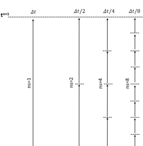
A subcycling technique was introduced in order to increase the computational time step and further speed the computa-tion up. Subcycling consists of setting a larger than the min-imum time step as a global time step1t, and making blocks with a smaller local time step cycle in substeps (ns) to match the global1t. The time step1tis calculated in each level us-ing the Courant–Friedrichs–Lewy condition (CFL) (Courant et al., 1967). Initially the CFL number is set to 0.8 for this work.
A graphical illustration of the subcycling implementation is shown in Fig. 14. Blocks with the same number of subcy-cles (levels L1–L4) are grouped in a single list. A block at level 5 (L5) has a time step of1t /2, which implies that it requires two cycles to match the global1t.
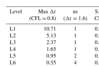
While in theory the larger time step increases speed, a po-tential downside is that too many blocks subcycling can cre-ate a large workload overhead, resulting in a slowdown of the whole computation. To avoid this, a global1t of 1.6 s is chosen to subcycle only blocks with levels over level 4. The reason being, is that around 80 % of the total number of mesh blocks are level 3 and subcycling them would repre-sent too large an overhead and would defeat the purpose of applying this technique. Table 1 gathers the CFL numbers per level after implementing the subcycling. The second column shows the maximum1t allowed in each level using the ini-tial CFL=0.8. The third column shows the resulting number of subcycles per level (ns) and the fourth column shows the new CFL values obtained for each level. In all cases the new CFL values remain below 1 to guarantee stability.
In general after a large1t step, corresponding boundary conditions are interpolated in time to update the substeps. However, this procedure introduces an additional compu-tational overhead. To pursue the fastest modeling possible, TRITON-G rescinds the boundary generation and instead uses the available boundary values at timen. Based on the benchmark and hindcast comparison, this decision proved to be acceptable based on the good agreement and accuracy of the results.
M. Arce Acuña and T. Aoki: Tree-based mesh-refinement GPU-accelerated tsunami simulator 2573
Figure 10.Indian Ocean domain partition for load balance for eight GPUs. Each color represents a different GPU.
Figure 11.Multi-GPU communication. GPU buffer data collected and packed for a single communication.
requires. This approach for the domain partition allows us to create a fair work rebalance on the GPUs. The effect of im-plementing the weighted load balance can be seen in Fig. 15, where GPU execution times per time step are presented, with and without load balance. Implementation of the subcycling technique showed a speedup of around 15 % in the total wall-clock runtime.
5.3.2 Runtime performance
Several tests to estimate the performance of TRITON-G were done. Results ran on the supercomputer Tsub-ame 3.0 (TsubTsub-ame, 2017) are presented, with Intel Xeon E5-2680 2.4 GHz×2, RAM 256 GB, NVIDIA Tesla P100
Table 1.CFL values used after introducing subcycling (S.C. CFL) for each of the seven levels. The second column shows the max-imum1t per level using CFL=0.8 and the third column shows the number of subcycles (ns) required in each level when using 1t=1.6.
Level Max1t ns S.C.
(CFL=0.8) (1t=1.6) CFL
L1 10.71 1 0.12
L2 5.13 1 0.25
L3 2.37 1 0.54
L4 1.65 1 0.78
L5 0.95 2 0.68
L6 0.55 4 0.59
L7 0.26 8 0.39
(16 GB)×4/node, CUDA 8.0, gcc 4.8.5, Openmpi 2.1.1 and Omni-Path HFI 100 Gpbs network.
As comparison, results on a second machine are also pre-sented using four Tesla K80 (12 GB×2) cards in a node (eight GPUs in total). GPUs are connected through PCI-Express 3.0, Intel Xeon CPU E5-2640 @ 2.6 GHz, RAM 128 GB, CUDA 8.0, gcc 4.7.7 and Openmpi 1.8.6. These per-formance tests serve to show very good portability of our pro-gram on different hardware, older and much newer, without requiring changes or producing problems.
Figure 12.TRITON-G computational flow; mem: memory.
Figure 13.Output overlap and optimization using Pipe.
Figure 14.Illustration of the subcycling process for each level.
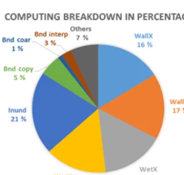
represents only 9 % of the total running time. It can be seen that the Wet and Wall kernels have similar performance de-spite the fact that the wall includes additional treatment for
Table 2.Kernel performance for one GPU in GFLOPS
Kernel GFLOPS
WallX 549.57 WallY 549.56
WetX 706.98
WetY 712.51
Inund 87.12
the coast boundaries. Since this treatment consists of many conditionals and they were replaced during optimization, it is understandable that the performance is similar. The slice Others includes several values; most importantly communi-cations which represents around 1.5 %–2.0 % of the total run-ning time. Performance of the main kernels on one GPU in floating point operations per second (FLOPS) is gathered in Table 2.
Results for runtimes using Tesla P100 cards and Tesla K80 cards are presented in Fig. 17 for one to four and eight GPUs. For this test, 10 h were simulated on the mesh initially gen-erated for the Indian Ocean domain (Fig. 5). All runtimes measurements include output time.
A comparison between both GPU cards shows a speed up of almost four times from the older K80 cards to the lat-est P100 on Tsubame 3.0. In our collaboration project with RIMES an objective to complete this test under 15 min was set, which could be fulfilled by using three to eight GPUs in this configuration. Runtime for three GPU with K80 cards was 39.96 and 12.1 min with P100 cards.
A saturation is noticeable in Fig. 17 as the number of GPUs are increased. A possible reason for this phenomenon is related to the increase of buffer preparation, packing– unpacking and the communication exchange. Using the same domain size for all cases is another possible reason. Hav-ing fewer blocks on each GPU generates lower occupancy which might degrade performance. However, having met this study’s time-to-solution objective of less than 15 min, no fur-ther optimization was deemed necessary.
M. Arce Acuña and T. Aoki: Tree-based mesh-refinement GPU-accelerated tsunami simulator 2575
Figure 15.GPU execution time with and without load balance.
Figure 16.Computing breakdown shown in percentage.
four GPUs for just 2 min wall-clock time is required to gener-ate the results of the inundation. The real tsunami wave took approximately 2 h to propagate from the initial source to Sri Lanka, obtaining simulation results faster than real time. This gives authorities sufficient time to make decisions regarding evacuations.
6 Tsunami inundation benchmark comparison
In order to compare the numerical results of TRITON-G with existing benchmarks and test its ability to estimate in-undation, we present the results obtained using the main benchmark tests proposed in the National Tsunami Haz-ard Mitigation Program workshop (NTHMP, 2012). Results from other models participating in the workshop can be con-sulted in that reference. In this section, the comparison of the
Figure 17.Wall-clock comparison of 10 h simulation on Tesla K80 and Tesla P100.
benchmark “1993 Hokkaido–Nansei–Oki (Okushiri) field” is shown. Further comparison results with benchmark prob-lems 4, 6 and 7 (abbreviated as BP4, BP6, BP7) can be found in the “Appendix”.
A detailed description of the benchmarks can be found in NTHMP (2012) and the data needed for them can be found in the repository https://github.com/rjleveque/ nthmp-benchmark-problems (last access: 13 September 2018). For completeness we give a brief explanation of the benchmark and the tasks it involves.
6.1 Benchmark problem no. 9: Okushiri Island tsunami – field
Figure 18. (a)Entire domain-refined mesh containing seven levels.(b)Zoom on Okushiri island. Higher resolution used around Monai Valley at level 7 (7 m approx.) and Aonae region at level 6 (14 m approx.).
6.1.1 Problem setup
The following parameters were used for the computation. – Bathymetry is taken from databases provided by
NTHMP (2012), interpolated where necessary. – The CFL is 0.9.
– The simulated time is 60 min.
– The initial condition is source generated from the database provided by the DCRC (Disaster Control Re-search Center) Japan solution DCRC17a, described in Takahashi (1996).
– The boundary conditions are open boundaries at the four domain edges.
– For friction, the Manning coefficient is set to 0.02. – For the computational domain, a mesh refinement is
used (shown in Fig. 18). Seven levels are used in total. The resolution of base level 1 is 450 m and the resolu-tion of level 7 is approximately 7 m. Dry blocks that did not take part in the computation were removed in the mesh generation process.
6.1.2 Tasks to be performed
This benchmark requires the following tasks to be per-formed:
1. compute run-up around Aonae;
2. compute arrival of the first wave to Aonae;
3. show two waves at Aonae approximately 10 min apart (the first wave came from the west, the second wave came from the east);
4. compute water level at Iwanai and Esashi tide gauges; 5. maximum modeled run-up distribution around Okushiri
island;
6. modeled run-up height at Hamatsumae; and 7. modeled run-up height at a valley north of Monai.
6.1.3 Numerical results
In this section we present the numerical results obtained with TRITON-G for benchmark problem no. 9.
Run-up around Aonae
The maximum inundation around Aonae peninsula modeled during the simulation is shown in Fig. 19. Contours every 4 m are drawn to show the outline of the topography. Maximum inundation height computed was nearly 15 m but the scale used is set to the upper limit of 10 m to highlight the areas where major inundation occurred.
M. Arce Acuña and T. Aoki: Tree-based mesh-refinement GPU-accelerated tsunami simulator 2577
Figure 19.Inundation map of Aonae region with 4 m contours of bathymetry and topography.
Figure 20.Arrival wave at Aonae peninsula coming from the west, snapshots of the wave at times 4.9 and 5.0 min after tsunami generation.
east side of the peninsula, deep penetration was found due to the flatter topography in this area. The inundation on the east side was mainly produced by the second wave coming from the east. The south side of the peninsula experienced the im-pact of both first and second waves and run-up of over 12 m was estimated.
Arrival of first wave to Aonae
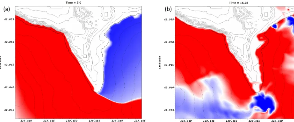
Figure 21. Two waves arriving at Aonae peninsula.(a)First wave coming from the west arrived at aroundt=5 min.(b)Second wave coming from the east arrived at aroundt=16 min.
Figure 22.Water level comparison between observations and TRITON-G results for Esashi(a)and Iwanai(b)tide gauges.
Two waves arriving at Aonae
The two waves arriving at Aonae peninsula are shown in Fig. 21. The first one came from the west (Fig. 21a) and made impact at around 5.0 min after the tsunami generation. The second major wave to hit the peninsula came from the east and made impact at around 16 min (Fig. 21b). Slightly over 10 min separated the first and second wave.
Tide gauge comparison at Iwanai and Esashi
sev-M. Arce Acuña and T. Aoki: Tree-based mesh-refinement GPU-accelerated tsunami simulator 2579
eral reasons. Inaccuracies in the source used for the initial condition can greatly influence the result. Additionally, the lack of realistic bathymetry including man-made structures around the area can affect the results as well.
Inserted in each panel of Fig. 22 are the estimated errors for the gauge comparison. The maximum wave amplitude error for Esashi station is 16.27 % and for Iwanai 3.19 %. These are considerably lower than the mean values obtained by the models reported in the workshop (NTHMP, 2012) of 43 % and 36 %, respectively. Although no values are reported in NTHMP (2012), the normalized root-mean-square devia-tion (NRMSD) error is also estimated for our model and in-cluded in the panels. Both values are under 20 %.
Maximum run-up around Okushiri
The computed maximum run-up distribution around Okushiri Island is shown in Fig. 23. Observations were taken from Kato and Tsuji (1994). Good agreement is found between observed and computed values around the coast. Most values are within the observed range or within a small difference from the field measurement. The simulation seems to capture well the variations that occurred along the coast.
The model could simulate well the maximum run-up ob-served around Monai valley within a reasonable 15 % error. The major differences are found in the southwest side of the island, where run-up values were underestimated with larger difference. The discrepancies could be explained by the use of different grid around the island coast. Additionally, the lack of an accurate high-resolution bathymetry database ev-erywhere can also influence the computed values as well as an inaccurate initial condition.
Run-up height at Hamatsumae
The maximum inundation map for Hamatsumae region is shown in Fig. 24. Topography and bathymetry contours are outlined every 4 m. A grid resolution of approximately 14 m was used for this region. Near the center of the region and to the east, run-ups of nearly 16 m were computed. Addition-ally, inundation values ranging from 8 to 10 m were obtained which match well with field observations.
Run-up height at a valley north of Monai
The maximum inundation map for the valley north of Monai is shown in Fig. 24. Topography and bathymetry contours are outlined every 4 m. A grid resolution of approximately 7 m was used for this region. Inundation of around 26 m was computed, relatively close to the 30.6 m observed in the field.
Figure 23.Computed and observed run-up values in meters along the coast of Okushiri island.
7 Case study
In order to compare and validate the results of TRITON-G under a real tsunami scenario we use the hindcast of the 2004 Indonesian tsunami. Results for propagation, gauges and inundation comparison are presented.
7.1 Indonesian 2004 tsunami hindcast
This event occurred at 07:58 LT on 26 December 2004, with a magnitude ofMw=9.0 generated by the subduction of the Indian plate by the Burma plate. Nearly 1600 km of fault was affected around 160 km off the coast of Sumatra (Titov et al., 2005). This massive earthquake generated a large tsunami that spread over the Indian Ocean in the following hours.
The tsunami wave propagation computed by TRITON-G is depicted in Fig. 26. Each subsequent snapshot represents 3 h after the earthquake’s main event. A synoptic qualitative comparison with existing field surveys and simulations con-firmed a correct propagation of the initial wave train; how-ever, to check the validity of the results, two kind of compar-ison are presented for tide gauge records and for inundation map simulations.
7.1.1 Tide gauge comparison
Figure 24.Inundation map of Hamatsumae region with 4 m contours of bathymetry and topography.
Figure 25.Inundation map for the valley north of Monai with 4 m contours of bathymetry and topography.
obtained through RIMES. Results from RIMES’ previous operational model are also included for comparison. Their previous model was based on a customization of TUNAMI (Srivihoka et al., 2014) to include four nested grids with fixed resolutions of 2 arcmin, 15 arcsec, 5 arcsec and approx-imately 1.67 arcsec.
Results for five stations are shown: Diego Garcia (Fig. 27a) in an atoll in the Chagos Archipelago, located at 7◦300N 72◦380E; Male (Fig. 27b) near the Maldives islands, located at 4◦180N 73◦520E; Gan (Fig. 27c) near the Maldives islands, located at 0◦680N 73◦170E; Colombo (Fig. 27d) in Sri Lanka, located at 64◦930N 79◦830E; and Point La Rue (Fig. 27e) near Seychelles, located at 4◦680S 55◦530E.
The comparison between the tide gauges TRITON-G and RIMES’ model based on TUNAMI are shown in Fig. 27. As it can be seen, the arrival times are in good agreement with the measured ones. The main event peaks are also
M. Arce Acuña and T. Aoki: Tree-based mesh-refinement GPU-accelerated tsunami simulator 2581
Figure 27. (a)Comparison of arrival wave at Diego Garcia, tide gauge and model results.(b)Comparison of arrival wave at Male, tide gauge and model results.(c)Comparison of arrival wave at Gan, tide gauge and model results.(d)Comparison of arrival wave at Colombo, tide gauge and model results.(e)Comparison of arrival wave at Point La Rue, tide gauge and model results.
traveled over complex bathymetry and reflected on multiple coastlines. However, the arrival time is still in good agree-ment as is the wave arrival peak height. No effect of wave main peak diffusion is noticeable.
The arrival time differences of a few minutes between measurement and TRITON-G simulation can be partly ex-plained by the location of simulated gauges. Even though the main events could be reproduced, a tendency to over-shoot is noticed; nonetheless, this did not affect the ability of the model to transport the wave along far distances, and in no case was an arrival wave sign reported incorrectly. We briefly discuss three main reasons for the difference in arrival height and wave oscillation after the main event. The first is related to bathymetry and topography. Although databases for bathymetry and topography with good accuracy are avail-able, these are still far from representing in detail the real shape of the ocean’s bottom and topography. This difference makes it challenging to reproduce the wave reflections on
M. Arce Acuña and T. Aoki: Tree-based mesh-refinement GPU-accelerated tsunami simulator 2583
Figure 28. Inundation comparison for Hambantota, Sri Lanka. (a)RIMES model.(b)TRITON-G model.
wave with a minimal dispersion effect is produced instead, reducing the possibility of seeing the higher oscillatory be-havior of the arrival tsunami wave seen in the gauges. These kinds of discrepancies had been observed and reported on in several other operational models as well (Dao and Tkalich, 2007; Grilli et al., 2007; Arcas and Titov, 2006).
7.1.2 Inundation map comparison
A further validation for the TRITON-G model is to com-pute inundation in certain areas and compare it with field surveys or existing maps. Since inundation maps that are ex-actly measured do not exist, we present comparisons with RIMES’ existing simulated inundation maps (RIMES, 2014) and post-tsunami field surveys. Two cases are presented: the first in Hambantota (Sri Lanka) and the second in Phuket (Thailand).
The first inundation validation presented is the result for Hambantota in Sri Lanka. The inundation map for Ham-bantota generated by TRITON-G is shown in Fig. 28b. For comparison, we include in Fig. 28a panel the previous re-sult obtained by RIMES in their report “Tsunami Hazard and Risk Assessment and Evacuation Planning – Hambantota, Sri Lanka” (RIMES, 2014).
Eyewitness accounts report the arrival time of the first tsunami wave around 09:00 LT the morning of the 26th, some 2 h after the initial earthquake in Sumatra. This coincides with TRITON-G’s predicted arrival time of 2 h for this re-gion. According to measurements done post-tsunami, it was
determined that the arrival waves had heights of over 8 m and produced run-ups inland in certain areas of up to 2 km.
TRITON-G inundation results also show areas up the coastal bay where run-up produced inundation hundreds of meters deep in land, coinciding with the recounts. By com-paring it with the result provided by RIMES, we found that both simulations show agreement with each other on the ar-eas that experienced and did not experience inundation. The decisive factor that made some areas more prone to inun-dation than others was the topography. The arrival tsunami wave hit the coast with heights of around 8–10 m. Coastal areas that faced the ocean with higher topographic heights were spared from being inundated. On the contrary, coast shores that were practically flat were overtaken by the in-coming wave as shown in the results.
Results for the second inundation validation in Phuket are compared with those of Supparsri et al. (2011). The wave arrival time for this region is of around 181 min, which agrees with the values obtained by TRITON-G model of 180 min. Inundation results are shown in Fig. 29, the im-age on top presents the inundation simulation obtained in the report while the image on the bottom depicts the results of TRITON-G model.
The results around the Kamala region coincide very well between models. Both report maximum inundation heights of around 5–6 m, and the run-up distances follow the same pattern. In the south, at Patong region however, there is a difference in the run-up distances. This is explained by the difference in the bathymetry used by TRITON-G. While in the Supparsri et al. (2011) study, a 52 m resolution was used on the entire inundation area, our model only used 50 m reso-lution bathymetry in Kamala. For Patong, values were inter-polated from a lower 150 m resolution database, which pro-duced a smoother topography and less accurate run-up re-sults. This highlights the importance and the effect of having accurate and realistic bathymetry for the simulation.
This test, together with the good results obtained in the in-undation benchmark comparisons (Sect. 6 and “Appendix”), served to validate the ability of TRITON-G to estimate tsunami inundation.
8 Conclusions
re-Figure 29. Kamala (north) and Patong (south) inundation maps comparison. (a) Inundation result by Supparsri et al. (2011). (b)TRITON-G inundation result.
finement that captured complex coastline shapes was suc-cessfully implemented using two factors; distance and focal areas. Using the distance from the coast to refine allowed us to leave coarser blocks in the open ocean, while blocks near the shoreline were refined to a higher 50 m resolution. Focal areas were also successfully introduced in the refine-ment to delimit the regions where the high-resolution blocks were generated and to use memory and computational re-sources efficiently. A full-GPU double-precision implemen-tation was proven successful in delivering a large increase in speed. All parts of this simulation, including output storage are processed entirely on GPU with specialized kernels. For multi-GPU, the use of a weighted Hilbert space-filling curve successfully generate balanced domain partitions and work-load.
Using Tsubame 3.0’s GPU Tesla P100 cards for a full-scale simulation of 10 h resulted on a wall-clock time of just under 10 min with three GPU cards, including considerably sized output (65 GB) while using double precision. The hind-cast of the Indonesian 2004 tsunami served to compare and validate TRITON-G simulation results, finding very good agreement with gauge propagation and inundations. Addi-tionally, good agreement with standard inundation bench-mark problems BP4, BP6, BP7 and BP9 was obtained. The flexibility and robustness of TRITON-G allows it to be an ex-cellent operational model that can be easily adjusted for dif-ferent tsunami scenarios, and its speed permits it to be a real-time forecasting tool. For these reasons, and under the col-laboration with RIMES, TRITON-G has been successfully deployed as their operational model since August 2017.
M. Arce Acuña and T. Aoki: Tree-based mesh-refinement GPU-accelerated tsunami simulator 2585 Appendix A: Benchmark problem no. 4: solitary wave
on a simple beach – laboratory
Numerical results for benchmarks 4, 6 and 7 are presented in this section. A detailed description of the problems can be found in NTHMP (2012). Here, we give a brief explanation in each section for completeness.
The domain for this test is shown in Fig. A1. In this problem, the wave height H is located at a distance L from the beach toe. This test was replicated in a wave tank 31.73 cm long, 60.96 cm deep and 39.97 cm wide at the Cal-ifornia Institute of Technology. Several experiments with different water heights were performed. Benchmark prob-lem 4 (BP4) uses the datasets for H /d=0.0185 non-breaking wave andH /d=0.30 breaking wave for code val-idation. Results use dimensionless units with the help of pa-rameters like length d, velocity scale U=√gd and time scaleT =√d/g.
A1 Problem setup
The following parameters were used for the computation. – Parameters: d=1 andg=9.8 in case A withH /d=
0.0185 and case B withH /d=0.30.
– Friction: the Manning coefficient is set to 0.01.
– Computational domain: the domain along x direction spans fromx= −20 tox=80.
– Boundary conditions: a non-reflective boundary condi-tion is used at the right side of the computacondi-tional do-main.
– Grid resolution: the numerical results presented are solved with a resolution of1x=0.1.
– CFL: the value is set to 0.9.
– Initial condition: the initial wave is computed based on the following equations for height (η) and velocity (u). η(x.0)=Hsech2
γ (x−xs) /d (A1)
u(x,0)= −η(x,0) r
g
d (A2)
A1.1 Tasks to be performed
To accomplish this problem, the following tasks should be performed.
1. Compare the numerically calculated surface profiles at t/T =30:10:70 for the non-breaking caseH /d= 0.0185 with the lab data (case A).
2. Compare the numerically calculated surface profiles att /T =15:5:30 for the breaking caseH /d=0.30 with the lab data (case C).
3. Compute the maximum run-ups for at least one non-breaking and one non-breaking wave case.
A1.2 Numerical results
We present the numerical results obtained using TRITON-G. Figure A2 shows the comparison between water surface level measured in the experiment and the modeled numerical results obtained by our model for times 30, 40, 50, 60 and 70 for case A (H /d=0.0185). Our results show good agree-ment between the numerical simulation and the non-breaking experiment.
Table A1 shows the errors computed for the NRMSD and for the maximum wave amplitude error (MAX). The er-ror values obtained by the NTHMP workshop models are also included for comparison. These values are divided into two columns: one with results for the non-dispersive mod-els (ND) and the other with results for the non-dispersive and dispersive models together (labeled ALL).
Errors obtained from our simulation tend to be similar or smaller than those errors obtained by other ND models, with just slight exception for time 70. Additionally, except for time 70 our errors are smaller than those obtained combin-ing non-dispersive and dispersive mean error values.
Water level comparison for case C (H /d=0.30) at times 15, 20, 25 and 30 is shown in Fig. A3. Table A2 gath-ers the values for NRMSD and MAX errors for our numerical results and for the NTHMP workshop models. In this case, only the results of models that reported their errors are in-cluded (taken from Tables 1–8, p. 41 in NTHMP, 2012).
For case C conditions, the shallow water equations are no longer appropriate for modeling and hydrostatic models tend to produce larger differences than non-hydrostatic ones. Our numerical results in general show good agreement with the experiment.
The difference with the steepening of the crest that is no-ticeable in the results is expected from a hydrostatic model. In spite of that, this steepening in our model is not very large and it can trace the wave front well. Once the wave breaking occurs, our model can simulate the run-up reasonably well. This is also partly reflected in the small NRMSD error esti-mation obtained by our model after the wave breaking.
Maximum run-up for case A and case C were calcu-lated. For the non-breaking case A, the obtained run-up value is 0.091, and for the breaking case C, the run-up estimated is 0.588. These values are plotted in Fig. A4 with a yellow and red dot, respectively. It can be seen that both values lie well within the experimental results.
A2 Benchmark problem no. 6: solitary wave on a conical island – laboratory