Hyperbolic Tangent ansatz method to space time fractional modified KdV, modified EW and Benney–Luke Equations

Hyperbolic Tangent ansatz method to space time fractional

modified KdV, modified EW and Benney–Luke Equations

Ozlem Ersoy Hepson∗

Eski¸sehir Osmangazi University, Department of Mathematics & Computer, 26200, Eski¸sehir, Turkey.

February 16, 2018

Abstract

The space time fractional Korteweg-de Vries equation, modified Equal Width equation and Benney-Luke Equations are solved by using simple hyperbolic tangent Ansatz method. A simple compatible wave transformation in one dimension is employed to reduce the governing equations to integer ordered ODEs. Then, the ansatz approximation is used to derive exact solutions. Some illustrative examples are presented for some particular choices of parameters and derivative orders.

Keywords: Ansatz method; fractional modified Korteweg–de Vries Equation; fractional modified Equal Width Equation; fractional Benney-Luke Equation; Conformable frac-tional derivative.

MSC2010: 35C07;35R11;35Q53.

PACS: 02.30.Jr; 02.70.Wz; 04.20.Jb

1

Introduction

Fractional calculus has been used in almost all fields of engineering, mathematics and other natural sciences. Recently, several mathematical methods have been applied to PDEs. Two-dimensional differential transform method was implemented to obtain ap-proximate analytical solutions of fractional modified Korteweg-de Vries(fmKdV) equa-tion [1]. Homotopy analysis method and its modificaequa-tion were used to solve fmKdV equation [2]. Similarly the homotopy-perturbation method was also capable of get-ting approximate analytical solution of fmKdV equation [3]. In [4], the travelling wave solutions were expressed in terms of hyperbolic, trigonometric and rational functions. Then (G0/G)-expansion method was applied for the analytical solutions of the fmKdV equations. Exact solutions of the fmKdV equation were investigated by the generalized Kudryashov method by Bulut et al. [5]. In that paper, soliton solutions and hyperbolic function solutions were constructed by using the properties of exponential functions.

∗

[email protected]

The conformable fractional mKdV equation

Dα_tu(x, t) +pu2(x, t)D_xβu(x, t) +qD_x3βu(x, t) = 0, (1)

where u is defined for x > 0, t > 0 and the coefficients p, q ∈ _R− {0}, is considered. In this equation, the conformal derivative operators Dxβ and Dtα represent the β.th and α.th order derivatives (β, α∈(0,1]).

The fractional modified Equal Width (fmEW) equation in conformable fractional form as

Dα_tu(x, t) +ru2(x, t)Dβ_xu(x, t) +sD_xtββαu(x, t) = 0 (2)

is also regarded as the second equation to be solved exactly forx >0, t >0. The bright soliton solutions and singular solutions were obtained using ansatz method when the derivatives are in sense of modified Riemann-Lioville derivative [7]. Hosseini and Ayati derived exact solutions of fmEW equation via the Kudryashov method. For this purpose, they introduced fractional complex transformation to reduce it into the integer ordered ordinary differential equation. Korkmaz introduced some more exact solutions in forms of various hyperbolic functions [6].

The space-time fractional Benney-Luke (fBL) equation in conformable fractional form can be interpreted as

D2_tαu(x, t)−D_x2βu(x, t) +µD4_xβu(x, t)

−ηD_xt2β2αu(x, t) +D_tαu(x, t)D2_xβu(x, t)

+2Dβ_xu(x, t)D_xtβαu(x, t) = 0 (3)

is considered as the last equation to be solved exactly, where x > 0, t >0 and µ and η

are positive parameters, linked to the inverse bond number, whose characteristics is to capture the effects of surface tension and the gravity forces [12]. This equation describes two-way water wave propogation in the presence of surface tension [9]. The existence and analyticicity of lump solutions for generalized Benney-Luke equations was proved by [8]. In [10], some travelling wave solutions of two well-known BL equations were derived via tanh-coth method analytically. An expansion method was applied to the BL equation for travelling wave solutions expressed by the trigonometric, hyperbolic and rational functions in [11]. Also, Kudryashov method and the modified extended tanh expansion were also applied for Benney-Luke equation [13].

This paper is organized as follows: In Section 2, Preliminaries and Essential Tools are given. In section 3, the ansatz method is mentioned briefly. Then, in Sections 4,5,6 the ansatz method is given for space–time fmKdv, fmEW and Benney–Luke equations, respectively. In the last sections,the findings are summerized.

2

Conformable Fractional Derivative and its Properties

Dα_t(u(t)) = lim

τ→0

u(t+τ t1−α)−u(t)

τ , α∈(0,1] (4)

in the positive half space for a function u : [0,∞) → _R [14]. The αth conformable derivative supports several properties given below.

Theorem 1 Let α ∈(0,1], and assume thatu and v areα-differentiable in the positive half plane (interval) t >0. Then,

• D_tα(au+bv) =aD_tα(u) +bD_tα(v)

• D_tα(tp) =ptp−α,∀p∈_R

• D_tα(λ) = 0, for all constant function u(t) =λ

• D_tα(uv) =uD_tα(v) +vDα_t(u)

• D_tα(u_v) = vD

α

t(u)−uDtα(v) v2

• D_tα(u)(t) =t1−α du_dt

for ∀a, b∈_R [15–17].

The conformable fractional derivative supports many significant properties like Laplace transform, Gronwall’s inequality, chain rule, various integration rules, exponential func-tion, and Taylor series expansion [17].

Theorem 2 Let u be an α-differentiable function in conformable sense. Also suppose thatv is differentiable in classical sense and is defined in the range of u. Then,

D_tα(u◦v)(t) =t1−αv0(t)u0(v(t)) (5)

3

Method of Solution

The implementation of the ansatz method can be achieved after reducing the fractional PDE

P1(u, Dαtu, Dβxu, Dααtt u, Dxxββu, D αβ

txu, ...) = 0 (6)

to an ODE of the form

P2(U, U0, U00, . . .) = 0 (7)

by using a compatible wave transformation. In the present study, we choose the wave transformation

u(x, t) =U(ξ), ξ =a(x

β

β −ν tα

to satisfy the compatibility of the conformable derivative. The next step is determination of the power B of the ansatz in the predicted solution

U(ξ) =AtanhBξ, A6= 0, B 6= 0 (9)

by substituting it into (7). Setting B = 1 results in the solution of Eq. (7) leads an algebraic system of equations to specify the relation among the parameters. The particular goal is to determine the parameters A,a and ν in terms of the others. Once the relations between the parameters are determined, the solution to (7) can be expressed explicitly. The particular goal is to determine the parameters in PDEs in terms of the original variables.

4

The solutions of the conformable fmKdV Equation

The wave transformation (8) reduces the fmKdV equation (1)

−aν d

dξU(ξ) +paU(ξ) 2 d

dξU(ξ) +qa 3 d3

dξ3U(ξ) = 0 (10)

Integrating this equation once gives

−aνU(ξ) +1

3paU(ξ)

3

+qa3 d 2

dξ2U(ξ) =K (11)

whereK is the constant of integration. Substituting the predicted solution (9) into (11) results in

−avA(tanh (ξ))B+ 1/3paA3(tanh (ξ))B3+

qa3A(tanh (ξ))BB21−(tanh (ξ))22

(tanh (ξ))2

−2qa3A(tanh (ξ))BB1−(tanh (ξ))2−

qa3A(tanh (ξ))BB1−(tanh (ξ))22

(tanh (ξ))2 =K

If we chooseB = 1, then the previous equation obtained as

1 3paA

3_{+ 2qa}3_A

(tanhξ)3+ −avA−2qa3Atanh (ξ) =K

Since the predicted solution is different from zero, the last equation is satisfied if only the coefficients of powers of the hyperbolic tangent function are zero. Thus,

1 3paA

3_{+ 2qa}3_{A = 0 (12)}

−avA−2qa3A = 0 (13)

Solution of this algebraic system forA,aand ν gives

A=±

r

−6q

p

v=−2qa2

for nonzero p, q and arbitrarily chosen a. Using these data, one can write the solution of (7) as

u1,2(ξ) =±

r

−6q

ptanh (ξ)

Returning the original variables gives the solution to the fmKdV(1) as

u1,2(x, t) =±

r

−6q

ptanh

a

xβ β + 2

qa2tα α

(15)

for nonzero p, q. This solution is the general form of hyperbolic tangent function type solution family. Choosing the parameters properly, many solutions in different charac-teristics covering complex ones can be generated.

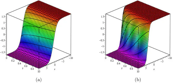
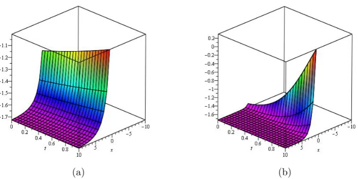
Some real solutions are illustrated for particular choices of the parameters. The effect of the derivative orderα andβ to the solution is indicated in the following figures. The solution (15) is chosen to demonstrate a particular solution by choosing the parameters asp= 2 andq =−1. The solutions are plotted onxtu−space for various values ofα,β

and a. Thus, the solution is reduced to

u(x, t) =−√6 tanh

a

xβ β −2

a2tα α

(16)

When the derivative order α = 0.5, β= 0.5, a= 0.5, the propagation of the wave is in Fig 1(a). When the derivative orderα= 0.5, β= 0.5, a= 1, the propagation of the wave is in Fig 1(b). When the derivative orderα= 0.5, β= 1, a= 0.5, the propagation of the wave is in Fig 2(a). When the derivative order α = 0.5, β = 1, a= 1, the propagation of the wave is in Fig 2(b). When the derivative order α = 1, β = 0.5, a = 0.5, the propagation of the wave is in Fig 3(a). When the derivative orderα= 1, β= 0.5, a= 1, the propagation of the wave is in Fig 3(b).

5

The solutions of the conformable fmEW Equation

The solution algorithm starts by transforming the fmEW to an ODE by using the com-patible wave transformation (8) . Thus, u(x, t) → U(ξ). This transformation reduces the fmEW (2) to

−aν d

dξU(ξ) +raU(ξ) 2 d

dξU(ξ)−sa 3_v d3

dξ3U(ξ) = 0 (17)

(a) (b)

Figure 1: (a)α= 0.5,β = 0.5,a= 0.5 (b) α= 0.5,β = 0.5,a= 1

(a) (b)

Figure 2: (a)α= 0.5,β = 1,a= 0.5 (b) α= 0.5,β = 1, a= 1

−avU(ξ) +1

3ra(U(ξ))

3_−sa3_v d2

dξ2U(ξ) =K (18)

(a) (b)

Figure 3: (a)α= 1,β = 0.5,a= 0.5 (b) α= 1, β= 0.5, a= 1

−avA(tanh (ξ))B+1 3raA

3_{(tanh (ξ))}B3₋sa

3_{vA(tanh (ξ))}B_B2_{1−(tanh (ξ))}22

(tanh (ξ))2

+2sa3vA(tanh (ξ))BB

1−(tanh (ξ))2

+

sa3vA(tanh (ξ))BB

1−(tanh (ξ))2

2

(tanh (ξ))2 =K (19)

B is determined as 1. Thus, the following equation is obtained as

1 3raA

3_−2sa3_vA

(tanh (ξ))3+ −avA+ 2sa3vA

tanh (ξ) =K (20)

Collecting the coefficients of powers of the tanh function yields to a system of algebraic equations inr, s, A, v, a, K of the form

1 3raA

3_−2sa3_{vA = 0 (21)}

−avA+ 2sa3vA = 0 (22)

K = 0 (23)

is obtained. Solving the resultant system (21-23) for {A, a, v, K}, the relation among these parameters are stated as

a = ±√1

2s (24)

v = 1 3rA

for arbitrarily chosenr, s. Thus, the solution to the equation (7) is determined as

u3,4(ξ) =Atanh (ξ) (26)

Returning the original variables (x, t) fromξ gives the solution to the EW(2) as

u3,4(x, t) =±Atanh

1

√

2s

xβ β −

rA2tα

3α

(27)

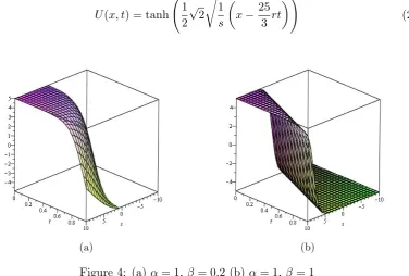
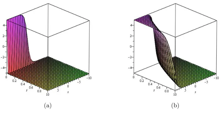
The plots of the solutions for some fixed values of the parameters (A= 5, r= 1, s= 1) When the derivative order α = 1, β = 0.2, the propagation of the wave is in Fig 4(a). When the derivative order α = 1, β = 1, the propagation of the wave is in Fig 4(b). When the derivative order α = 0.2, β = 1, the propagation of the wave is in Fig 5(a). When the derivative order α= 0.8, β= 1, the propagation of the wave is in Fig 5(b).

U(x, t) = tanh 1 2

√

2

r

1

s

x−25

3 rt

!

(28)

(a) (b)

Figure 4: (a)α= 1, β= 0.2 (b) α= 1, β= 1

6

The solutions of the conformable fBL Equation

The wave transformation (8) reduces the fBL equation (3)

a2(ν2−1) d

2

dξ2U(ξ) +a

4_(µ−ηv2₎ d4

dξ4U(ξ)−3a 3_v d

dξU(ξ)

d2

dξ2U(ξ) = 0 (29)

Integrating this equation once gives

a2(ν2−1)d

dξU(ξ) +a

4_(µ−ηv2₎ d3

dξ3U(ξ)−

3 2a

3_v( d

(a) (b)

Figure 5: (a)α= 0.2,β = 1 (b)α= 0.8,β = 1

whereK is the constant of integration. Substituting the predicted solution (9) into (3) results in

a2Atanh(ξ)BBv2

tanh(ξ) −a

2_vtanh(ξ)B_Btanh(ξ)v2₋a2Atanh(ξ)BB

tanh(ξ)

+a2Atanh(ξ)BBtanh(ξ) +a

4_µAtanh(ξ)B_B3_{(1−tanh(ξ)}2₎3

tanh(ξ)3

−6a

4_µAtanh(ξ)B_B2_{(1−tanh(ξ)}2₎2

tanh(ξ) −

3a4µAtanh(ξ)BB2(1−tanh(ξ)2)3 tanh(ξ)3

+4a4µAtanh(ξ)BBtanh(ξ)(1−tanh(ξ)2) + 4a

4_µAtanh(ξ)B_{B(1−tanh(ξ)}2₎2

tanh(ξ)

+2a

4_µAtanh(ξ)B_{B(1−tanh(ξ)}2₎3

tanh(ξ)3 −

a4ηv2Atanh(ξ)BB3(1−tanh(ξ)2)3 tanh(ξ)

+6a

4_ηv2_Atanh(ξ)B_B2_{(1−tanh(ξ)}2₎2

tanh(ξ) +

3a4ηv2Atanh(ξ)BB2(1−tanh(ξ)2)3 tanh(ξ)3

−4a4ηv2Atanh(ξ)BBtanh(ξ)(1−tanh(ξ)2)

−4a

4_ηv2_Atanh(ξ)B_{B(1−tanh(ξ)}2₎

tanh(ξ) −

2a4ηv2Atanh(ξ)BB(1−tanh(ξ)2)3 tanh(ξ)3

−3

2

a3vA2(tanh(ξ)B)2B2(1−tanh(ξ)2)2 tanh(ξ)2

= K

−6a4µA+ 6a4ηv2A−3

2a

3_vA2

tanh(ξ)4

+ a2A−8a4ηv2A+ 8a4µA−a2Av2+ 3a3vA2

tanh(ξ)2

+a2Av2−3

2a

3_vA2_−a2_A−2a4_{µA+ 2a}4_ηv2_A

= K

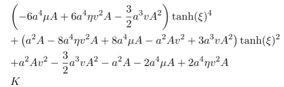
Since the predicted solution is different from zero, the last equation is satisfied if only the coefficients of powers of the hyperbolic tangent function are zero. Thus,

−6a4µA+ 6a4ηv2A−3

2a

3_vA2

= 0 (30)

a2A−8a4ηv2A+ 8a4µA−a2Av2+ 3a3vA2 = 0 (31)

a2Av2−3

2a

3_vA2_−a2_A−2a4_{µA+ 2a}4_ηv2_{A−K = 0 (32)}

Solution of this algebraic system forA,aand ν gives

A = ± 4(−µ+η)a

(4a2_η−1)q₋1−4a2µ 4a2_η−1

(33)

v = ±

s

−1−4a 2_µ

4a2_η−1 (34)

for nonzero µ, η and arbitrarily chosen a. Using these data, one can write the solution of (7) as

u5,6,7,8(ξ) =±

4(−µ+η)a

(4a2_η−1)q₋1−4a2µ 4a2_η−1

tanh(ξ)

Returning the original variables gives the solution to the space-time fractional BL equa-tion (3) ) as

u5,6,7,8(x, t) =±

4(−µ+η)atanh(ax_ββ ±q−1₄−_a24_η−a2µ₁t

α

α

)

(4a2_η−1)q₋1−4a2µ 4a2_η−1

(35)

This solution is the general form of hyperbolic tangent function type solution family. Choosing the parameters properly, many solutions in different characteristics covering complex ones can be generated.

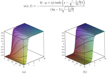
is in Fig 6(b). When the derivative order α = 1, β= 0.2, a= 5, the propagation of the wave is in Fig 7(a). When the derivative orderα = 1, β = 1, a= 5, the propagation of the wave is in Fig 7(b).

u(x, t) =−

4(−µ+η) tanhx−q−1₄−_η−4µ₁t

(4η−1)

q

−1₄−_η−4µ₁

(36)

(a) (b)

Figure 6: (a)α= 0.2,β = 1,a= 1 (b)α= 0.8,β = 1,a= 1

(a) (b)

7

Conclusion

Some conformable space–time fractional PDEs are solved by taking hyperbolic tangent ansatz. FmKdV, fmEW and fBL equations are reduced to some nonlinear ODEs of integer order by using compatible wave transformations. Substituting the solution into the resultant ODEs and finding relations between the parameters of the equations give the exact solutions of PDEs. The exact solutions are successfully found for particular choices of theαandβand the other parameters.As a conclusion, the method is applicable to PDEs in the theory of fractional calculus.

References

[1] Kuralay, M., Bayram, M. (2010). Approximate analytical solution for the fractional modified KdV by differential transform method. Commun Nonlinear Sci Numer Simulat 15, 1777–1782.

[2] Abdulaziz, O., Bataineh, A. S., Hashim, I. (2009) On convergence of homotopy analysis method and its modification for fractional modified KdV. J Appl Math Comput 33, 61–81. equations

[3] Abdulaziz, O., Hashim, I., Ismail, E.S. (2009). Approximate analytical solution to fractional modified KdV equations. Mathematical and Computer Modelling 49, 136–145.

[4] Wang, M., Li, X., Zhang, J. (2008). The (G/G )-expansion method and travelling wave solutions of nonlinear evolution equations in mathematical physics. Physics Letters A 372, 417–423.

[5] Bulut, H., Pandir, Y., Demiray, S. T. (2014). Exact Solutions of Time-Fractional KdV Equations by Using Generalized Kudryashov Method. International Journal of Modeling and Optimization, 4(4), 315-320.

[6] Korkmaz, A. (2017). Exact solutions of space-time fractional EW and modified EW equations. Chaos, Solitons and Fractals 96, 132–138.

[7] Hosseini, K., Ayati, Z. (2016). Exact solutions of space-time fractional EW and modified EW equations using Kudryashov method. Nonlinear Sci. Lett. A, 7(2), 58-66.

[8] Quintero, J. R. (2002). Existence and analyticity of lump solutions for generalized Benney-Luke equations. Revista Colombiana de Matematicas, 36, 71-95.

[10] Gozukızıl, O. F. and Akca˘gıl, S. (2012). Travelling Wave Solutions to the Benney-Luke and the Higher-Order Improved Boussinesq Equations of Sobolev Type. Ab-stract and Applied Analysis. 890574, 1-10.

[11] Islam, R. S. M. (2015). Applications of the exp(φ)-Expansion Method to Find Exact Traveling Wave Solutions of the Benney-Luke Equation in Mathematical Physics. American Journal of Applied Mathematics, 3(3), 100-105.

[12] Khan. U., Ellahi, R. Khan, R., Mohyud-Din S. T. (2017). Extracting new solitary wave solutions of Benny–Luke equation and φ-4 equation of fractional order by using (G/G)-expansion method. Opt Quant Electron (2017) 49, 362.

[13] Ali, K. K., Nuruddeen, R.I. (2017). Analytical treatment for the conformable space-time fractional Benney-Luke equation via two reliable methods, International Jour-nal of Physical Research, 5(2), 109–114.

[14] Khalil, R., Al Horani, M., Yousef, A., & Sababheh, M. (2014). A new definition of fractional derivative. Journal of Computational and Applied Mathematics, 264, 65-70.

[15] Atangana, A., Baleanu, D., & Alsaedi, A. (2015). New properties of conformable derivative. Open Mathematics, 13(1), 1-10.

[16] C¸ enesiz, Y., Baleanu, D., Kurt, A., & Tasbozan, O. (2016). New exact solutions of Burgers’ type equations with conformable derivative. Waves in Random and Complex Media, 1-14.