Visualizing Uncertainty in Geo-spatial Data

(1)

Visualizing Uncertainty in Geo-spatial Data

Alex Pang

Computer Science Department

University of California, Santa Cruz

[email protected]

September 20, 2001

This paper focuses on how computer graphics and visualization can help users ac-cess and understand the increasing volume of geo-spatial data. In particular, this paper highlights some of the visualization challenges in visualizing uncertainty associated with geo-spatial data. Uncertainty comes in a variety of forms and representations, and require different techniques for presentation together with the underlying data. In general, treating the uncertainty values as additional variables of a multivariate data set is not always the best approach. We present some possible approaches and further challenges using two illustrative application domains.

1 INTRODUCTION

There are many potentially exciting commercial and scientific applications that can be realized with the affordability and miniaturization of geo-location devices, ranging from advertisement of nearby establishment sent to your hand-held devices, to track-ing of disposable air-borne sensors for weather applications and miniature cameras ingested into our blood stream to study internal organs. As these components become more affordable and widespread, and as the volume and richness of geo-spatial data set being collected increase, the need for visualizing these data in an informative and consistent manner become more acute. In particular, there will inevitably be more con-cern about the accuracy, timeliness, and confidence of information being displayed – specially if the data are coming from multiple sources, or by their nature of collection contain some inherent uncertainty. We discuss the challenges of visualizing uncertainty in geo-spatial data sets in the context of two application domains, and also point out that existing visualization techniques, including multivariate and multi-dimensional vi-sualization techniques, are not adequate to address the expected stream of geo-spatial data and the need to visualize their associated uncertainty.

Uncertainty in geo-spatial data can be found in a number of sources and applica-tions such as weather forecasting, data assimilation, EOS data, to name a few. This

0_{This paper, prepared for a committee of the Computer Science and Telecommunications Board, should}

(2)

paper will focus on two specific examples for the purposes of presenting the state-of-the-art in visualizing uncertainty and identifying the research challenges. The first application starts with ocean modeling and leads to a number of different products, while the second one focuses on potential uses of EOS data.

In ocean modeling, uncertainty is often associated with variability. But it can also arise in different forms such as sparsity in data, noise in measurements, uncertainty in the model, etc. With multi-spectral EOS data sets, uncertainty can arise from mea-surement, registration, and calibration operations, but also from processing of the data themselves. For example, in earth sciences, derived quantities, such as “net primary productivity” [16], are derived in conjunction with remote sensing data and ecological models; conditional simulations [8] may use EOS or other remotely sensed data to pro-duce multiple realizations of land cover information, etc. In these instances, uncertainty may be represented in different ways such as scalar, intervals, tuples, or distributions at each geo-spatial coordinate. Different visualization techniques must be developed to present these uncertainty representations together with the underlying data.

2 UNCERTAINTY

In this section, we discuss some of the concepts of uncertainty used in literature. Be-cause the definition will have a direct impact on how uncertainty is represented, and hence visualized, we also identify a generic set of uncertainty representations.

2.1 Definitions

Many definitions of uncertainty have been proposed [1, 12, 17, 20, 23, 27]. Uncertainty is a multi-faceted characterization about data, whether from measurements and obser-vations of some phenomenon, and predictions made from them. It may include several concepts including error, accuracy, precision, validity, quality, variability, noise, com-pleteness, confidence, and reliability. The following non-exhaustive selection of pa-pers that discuss uncertainty imply that there is no consensus or universally recognized meaning for uncertainty.

1. In geographic information science, several recent works have been devoted to concepts related to uncertainty. The following definitions are proposed. Error can be defined as the discrepancy between a given value and its true value [12].

Inaccuracy is the difference between the given value and its modeled or

simu-lated value [12]. Validity encompasses both the accuracy of the data themselves and the procedures applied to the data. Data validity is measured by deductive estimates, inferential evidences, data consistency and comparison with indepen-dent sources and it is ratified by testing [12, 20]. Data quality is treated as an even more general term that includes data validity and data lineage. Data lin-eage refers to those characteristics of data that are monitored and tracked in database operations. Data quality can be defined as a three parameter variable,

(3)

that consists of goodness or statistical measure, application or model resolution, and purpose such as analysis or communication [1]. Data noise is an uncorre-lated and independent random error introduced in the data usually due to some background phenomenon such as atmospheric radiation, for example.

The NCGIA initiative on “Visualizing the Quality of Spatial Information” [1] classified the sources of data uncertainty as source errors, process errors and use errors. There are different sources of error that arise from the transformations that are applied from the data collection through the visualization stages. The data acquisition stage involves the capture of physical phenomena recorded ei-ther through sensors or as output from numerical or geometric models. These measured or predicted phenomena may undergo further transformations to pro-duce derived data. Typical transformations include data interpolation or approx-imation and data sampling or quantization. The derived data are then input to different visualization algorithms that generate images for the users to analyze. Any of these stages may affect uncertainty about the data.

In [23], spatial uncertainty is defined for both attribute values and position. It includes accuracy, statistical precision and bias in initial values, as well as in estimated predictive coefficients in statistically calibrated equations used in the analysis. “Most importantly, spatial uncertainty includes the estimation of errors in the final output that result from the propagation of external (initial values) uncertainty and internal (model) uncertainty.”

2. NIST [27] formulated guidelines for expressing the uncertainty of measurements. Measurement uncertainty, although consisting of several components, can be broadly classified into categories according to the method used to estimate its numerical values: 1) evaluation by statistical methods such as standard deviation and least squares techniques and 2) evaluation by scientific judgment such as including previous measurements, manufacturer’s specifications and experience. Combined data uncertainty is then computed to handle the propagation of un-certainty. Expanded uncertainty is derived by including confidence intervals and coverage factors, which again depend upon the level of confidence in the data. 3. Draper [6] frames the definition in the context of unknown quantitiesinferred

or predicted on the basis of known quantities. The model formalizes as-sumptions about howandare related. Uncertainty about predictions there-fore includes both uncertainty about the form of (structural uncertainty) and the parameters of (parametric uncertainty). The latter is the focus of most statistical practice while structural uncertainty has been mostly neglected. 4. While refraining from giving a succinct definition of spatial uncertainty, [3]

devote an entire text to geostatistical models of spatial uncertainty. These in-clude the quantification of the precision of interpolated estimates as well as the use of Monte Carlo simulation to describe multiple possible maps which, to-gether, describe a range of plausible spatial outcomes given some observed data.

(4)

Goovaerts [13] calls the first type of uncertainty local and the second type

spa-tial.

5. More recently, Klir and Wierman [17] state that uncertainty itself has many forms and dimensions and may include concepts such as fuzziness or vagueness, dis-agreement and conflict, imprecision and non-specificity.

6. In 2000, a Departmental Research Initiative (DRI) from the Office of Naval Re-search (ONR) requested proposals to capture uncertainty. In October of that year, a workshop was held to further define the research focus and possible ap-proaches. The results of the workshop are posted at

http://www.onr.navy.mil/sci_tech/chief/cuwg/index.html Uncertainty was defined to be related to the environmental variability that might be knowable and that we might simulate, the environmental variability that might be knowable but that we can not simulate, the environmental variability that is not knowable, and the error inherent in representations and calculations of the environmental field, acoustic field, and target estimation. The following mathe-matical definition of uncertainty was presented at the workshop in order to initi-ate and further discussion.

= estimated value of some quantity (measured, predicted, calculated ..) = actual value (unknown truth or unknown nature)

=-

The uncertainty incan be represented by the probability density function (pdf) of. The pdf need not be normal, have a mean of zero, or uni-modal.

There was also discussion that uncertainty is not the same as variability (of the environment), but that in most naval applications uncertainty refers to variability.

2.2 Representations

The short list above makes it clear that there are several concepts associated with un-certainty. Depending on which concept is being used, there may also be more than one way to represent and quantify the amount or nature of uncertainty. The manner in which uncertainty is represented is important for the task of visualizing data with uncertainty. Without over-simplifying and trivializing the problem, we can focus on the subset of uncertainty that are numerically represented by scalars, pairs or n-tuples, and as distributions.

Scalars are often used to quantify uncertainty concepts such as confidence levels, errors or differences, likelihood, etc. Pairs of scalar values on the other hand are more typical of intervals or ranges, but could also be value pairs such as mean and standard deviation. The next generalization is for n-tuples, for example, to represent the likeli-hood for a set of states or values of membership functions, as well as more elaborate

(5)

parametric statistical descriptions. In situations where sufficient sampling is available, the distribution itself may represent the uncertainty in the data.

These uncertainty representations call for different visualization techniques. Obvi-ously, scalars are the simplest to tackle, with difficulty in both visualization and feature extraction tasks increasing in direct proportion to the richness in which uncertainty is represented. In the next section, we review some of the efforts in visualizing uncer-tainty and highlight some of the key challenges.

3 VISUALIZATION CHALLENGE

3.1 Background

There is more than one way to classify how uncertainty can be visualized. One is by how uncertainty itself is represented, another is by how uncertainty is encoded into vi-sualization. For the latter, there are two general ways of combining uncertainty into a visualization: (a) mapping uncertainty information as an additional piece of data, and (b) creating new visualization primitives and abstractions that incorporate uncertainty information. The first method incorporates uncertainty information into the visualiza-tion by mapping it as transparency, haze, blur, etc. to alter the appearance of the under-lying data. On the other hand, the second method modifies the visualization primitive itself so that uncertainty can be encoded with the data, and usually in such a way that the interpretation of both data and uncertainty cannot be visually separated. We discuss examples of these two types next. Elaboration and additional information are provided in [24].

Uncertainty is an important issue with geospatial data sets, and hence it is not sur-prising to see a large number of papers from related fields such as geography and cartography. Some of the ideas presented include:

Mapping uncertainty to graphics attributes. Attributes of graphics primitives include

things such as: color, transparency, line width, and sharpness or focus. Examples that fall under this category include: varying contour widths depending on certainty [9], mapping uncertainty parameters to different points in HSV space [18], using cross hatches [21], including fog (amount of haziness corresponds to amount of uncertainty) and focus (amount of blurring corresponds to amount of uncertainty) [1], using trans-parency to indicate confidence in an interpolated field [25], and perturbing and blurring overlaid grid lines [2].

Using animation to convey uncertainty. Within the context of visualizing uncertainty,

Monmonier [22] created and played back sequenced images stored as graphics scripts. Similarly, MacEachren [19] used sequential presentation, including interactive anima-tion, as one of the methods for presenting uncertainty. Another approach proposed by [10] uses real-time animation of random dots to show uncertainty in spatial informa-tion. Similarly, [11] used animation loops to examine the role of motion detection in

(6)

visualizing fuzzy ranges of data values.

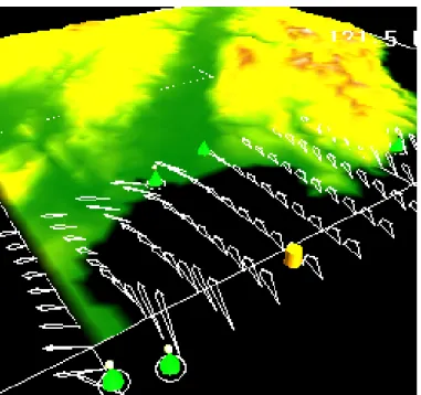
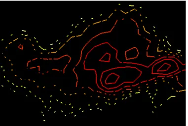
Most of the examples mentioned above treat the uncertainty as another variable or piece of information that need to be displayed. Hence, the resulting visualizations has a tendency to treat the uncertainty as another “layer” of information that need to be added e.g. as a transparency map, etc. An alternative approach is to treat the uncertainty as an integral, non-separable piece of information from the data, and thereby requiring visualization techniques that show both the data and its uncertainty in a holistic fash-ion. To illustrate this point, Figure 1 shows uncertainty glyphs for depicting angular uncertainty in vector fields, while Figure 2 shows how spatial uncertainty is naturally encoded by broken contour lines.

Figure 1: Uncertainty glyphs replace arrow plots or hedgehogs for depicting vector fields. The width of the glyph head corresponds to angular uncertainty. The veloc-ity magnitude is mapped to the area coverage of the glyph above. (Alternatively, it could be mapped to length as usual. But that mapping draws attention to areas with large magnitude and large uncertainty). Uncertainty in velocity magnitude can also be encoded as additional arrow heads showing min/max values (not shown above).

This is by no means an exhaustive list, but it gives a flavor of what has been pro-posed. This brings us to the challenges of visualizing uncertainty in geospatial data sets.

(7)

Figure 2: Spatial uncertainty is encoded as gaps in contour lines. The more uncertain, the larger the gaps. The contour lines themselves are for some other variable such as temperature, humidity, etc.

3.2 Challenges

The difficulty of visualizing data with uncertainty increases with the richness in which uncertainty is represented (from scalars to distributions) and the dimensionality of the data. As more information need to be displayed, it is natural to turn to techniques from multivariate and statistical visualization techniques such as Chernoff faces, scat-ter plots, star plots, box plots, etc. An excellent survey on multivariate and multi-dimensional visualization techniques can be found in [4].

It should be noted that multivariate and multi-dimensional refer to different things although their usage may overlap at times. Multi-dimension refers to the spatial orga-nization of the data within the space in which it resides. Specifically, 0-dimensional for scattered points even if they are within a 3D physical domain, 1-dimensional for curves, 2-dimensional for surfaces, 3-dimensional for volumes, etc. Dimensionality refers to the density or number of neighboring points at each data location. Multivariate refers to the number of variables present at each of these n-dimensional locations. Hence, the techniques in [4] referred to as being multi-dimensional, are in fact multivariate visualization techniques. For example, parallel coordinates [14] has been referred to as both a multidimensional and multivariate technique. It essentially maps an n-tuple data from some m-dimensional space onto a 2D projection where each of the n variables are layed out as parallel axes on 2D, and one searches for patterns on this projection. Of course, each of the m-dimension can be encoded as components of the n-tuple data.

Current multivariate techniques are mostly glyph-based and can support very low spatial dimensionality. Their ability to carry and present additional information such as uncertainty are quickly exhausted. So, there has also been proposals on using other

(8)

scalar pair n-tuple distribution

0D glyph glyph glyph histogram

1D modified contour box plot ? stacked histograms

2D transparency, fog, isosurface pair, ? see Section 5

texture, etc. animation

3D see Section 4 ? ? ?

... ? ? ? ?

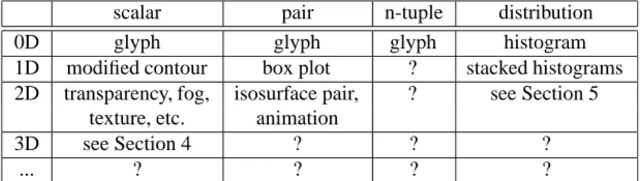
Table 1: Dimensionality versus uncertainty representation. Representative visualiza-tion techniques are listed while combinavisualiza-tions that need further research are filled with ?. Note that multivariate visualizations methods can be used for n-tuple representa-tions by treating spatial dimensions of data points as additional variables. In this case, locality information may be obscured.

modalities such as animation, sound, and force feedback to convey the additional infor-mation to the users. This is certainly worth pursuing although the bandwidth of these other channels are less than the visual means.

Table 1 provides one way of looking at what visualization techniques are available for uncertainty visualization and where we can focus our research efforts. As both data dimensionality and richness in uncertainty representation increase, there is more opportunity and challenge for creating effective visualization techniques.

The next two sections describe two applications with uncertainty in geo-spatial data sets. They also describe some of the difficulties faced in filling Table 1.

4 OCEAN MODELING

The quality of ocean modeling is dependent upon a number of factors including model resolution, initial and boundary conditions, completeness of physical modeling, etc. Uncertainty is often used inter-changeably with variability. It is inherently spatial in nature in that some regions of the ocean may exhibit higher variability than others.

This section describes some initial attempts at visualizing 3D scalar uncertainty in ocean models. The data set is from the numerical ocean model of the Harvard Ocean Prediction System [26], and includes physical variables such as temperature, salinity, velocity and pressure. Monte Carlo simulations are carried out to generate a 3D ensemble of the ocean state. The simulations are based on ocean data collected in the Middle Atlantic Bight (MAB) south of New England. The dominant feature in the MAB consists of a temperature and salinity front, separating the shelf and slope water masses. The front is located above the shelfbreak, tilted, in the opposite direction of the bottom slope. For this endeavor, we utilize the variance of the Monte Carlo ensemble as a scalar representation for uncertainty at each point.

The idealized visualization problem then is to visualize a 3D field with a scalar

(9)

data uncertainties (a) data uncertainties (b) opacity uncertainty (c)

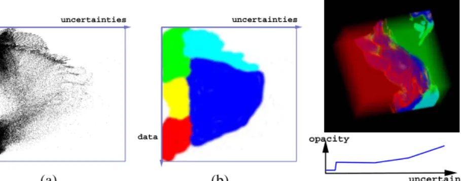
Figure 3: (a) Scatter plot. Mean salinity values increase towards the bottom, while un-certainty values increase towards the right. (b) Scatter plot used as a 2D transfer func-tion to identify 5 different regions. (c) Volume rendering with uncertainty-to-opacity mapping.

uncertainty at each point, e.g. mean temperature and variance of temperature at each point, or mean salinity and variance of salinity at each point.

Direct volume rendering is the method of choice for the visualizing a scalar 3D volumetric data. The scalar values are mapped to color and opacity using a 1D transfer function which dictates what opacity values and what color values to use given a scalar data value. At every pixel of the resulting image is an integration of the data values in the volume along the line of sight from the viewpoint. In [5], several modifications to the direct volume rendering algorithm were proposed so that scalar uncertainty values can be incorporated in the volume rendering. Here, we describe one of the proposed methods.

Figure 3(a) shows the scatter plot of the mean salinity values versus the variance in the salinity values. This scatter plot can be used as a 2D transfer function to specify what color values to assign to different data and uncertainty value pairs as illustrated in Figure 3(b). Figure 3(c) shows the resulting volume rendered image using this modified transfer function. In addition, opacity can be used to further emphasize the location and magnitude of uncertainty. This can be achieved by a simple 1D transfer function that maps uncertainty to opacity values.

While Figure 3(c) clearly shows where data of low salinity, low uncertainty (green), high salinity, low uncertainty (red), and high uncertainty (cyan and blue) are located through the use of color, it should be noted that the results may not always be this dramatic. In particular, this data set is centered over the shelf break where there is a distinctly higher variability in salinity and temperature giving rise to the nice separation in the scatter plot in Figure 3(a). In general, finding these delineations may not be as straight forward. Better, more robust ways of presenting 3D scalar uncertainties need to be pursued. Furthermore, instead of using a simple scalar (variance) to represent

(10)

uncertainty, what if one wants to use the Monte Carlo ensemble? How would one go about visualizing this type of data where one has a distribution at each 3D voxel? Towards this end, we look at a slightly simpler problem where one has a distribution of values at each 2D pixel. This is discussed in the next section.

5 EOS DATA

Data from many applications can be represented as a 2D field where each data point is a distribution. One example is data from the Earth Observing System (EOS) where one treats the spectra at each pixel as a distribution of data values. Another example is from remote sensing where one attempts to classify the land cover type for each pixel. In this case, the output from the classification algorithms may assign different percentage or probability that the pixel belongs to a particular class. The collection may then be treated as some sort of distribution. When faced with this type of data, previous visualization technique are relatively simple and typically reduce the distribution values down to a single value per pixel (e.g. [28]).

In this section, we highlight some of the techniques and challenges in visualizing 2D distribution data sets as reported in [15]. One of the data sets used is generated us-ing conditional co-simulation usus-ing both ground measurements and coincident satellite imagery. The ground measurements are of forest cover from 150 different locations throughout a region, while the imagery is from Landsat of a spectral vegetation index. Conditional simulation, also called stochastic interpolation, is one way to model uncer-tainty about predicted values in a spatial field [7, 8]. It is a process by which spatially consistent Monte Carlo simulations are constructed given some data and assumptions. Conditional simulation algorithms yield not one, but several maps, each of which is an equally likely outcome from the algorithm. Each equally likely map is called a real-ization. Taken jointly, these realizations describe the uncertainty space about the map. That is, the density estimate (e.g. histogram) of the data values is a representation of the uncertainty at each pixel.

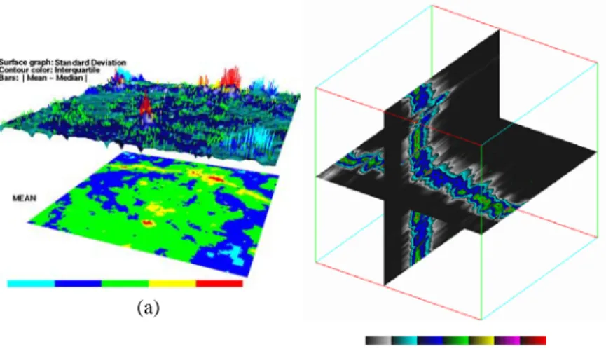
The visualization task is then to look at the 2D field and somehow get a sense of the uncertainty over the domain. One way is to simply plot the histogram of the distribution for every pixel. The obvious drawback to this approach is the screen res-olution requirement, and the ability of the user to digest such a potentially very busy and cluttered presentation. Another approach, shown in Figure 4(a), is to summarize each distribution into a smaller set of meaningful values that are representative of the distribution. Here, parametric statistics such as mean, standard deviation, kurtosis, skewness, etc. are collected about each distribution. This forms an n-tuple of values for each pixel that can then be visualized in layers. However, there are drawbacks to this approach as well. Namely, the limited number of parameters that can be displayed, the loss of information about the shape of the distributions, and the poor representa-tions if the distribution cannot be described by a set of parametric statistics. Clearly, alternative non-parametric methods need to be pursued.

(11)

Figure 4(b) allows the user to view parts of the 2D distribution data as a col-ormapped histogram. Here, the frequency of each bin in a histogram is mapped to color, thereby representing each histogram as a multi-colored line segment. A 2D dis-tribution data is then represented by a 3D histogram cube. Figure 4(b) shows 2 slices of this histogram cube depicting the relatively uni-modal distribution of the points on the two slices. Interactivity helps in understanding the rest of the field, but there is still the need to be able to “see” the distribution over the entire 2D field at once.

(a)

(b)

Figure 4: (a) The bottom plane is the mean field colored from non-forest (cyan) to closed forest (red). The upper plane is generated from three fields: the bumps on the surface is from the standard deviation field and colored by the interquartile range; and the heights of the vertical bars are from the absolute value of the difference between the mean and median fields colored according to the mean field on the lower plane. Only difference values exceeding 3 are displayed as bars to reduce clutter. (b) Histogram cube. Two slices of the volume depicts the histogram of each point along two lines across the 2D field. We can see that the distributions are mostly uni-modal and skewed towards lower values.

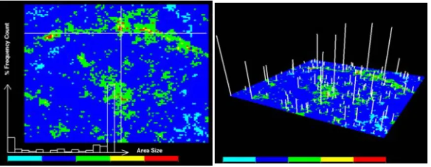
Beyond looking at distributions for each pixel, scientists also want to study features in these kind of data sets. For example, for each pixel, what is the size of the clump with similar classification as the pixel. Furthermore, what is the variability of this clump area size for the different realizations. Figure 5 illustrates some ways of providing this information to the user. It also emphasizes the need for interactivity as the data complexity goes up.

(12)

(a) (b)

Figure 5: (a) Interactive probing. The histogram on the bottom shows the distribution of different clump area size that contains the pixel under the cross-hair. (b) The top 166 clump areas that contain pixels in the current realization.

6 SUMMARY

In summary, visualizing the uncertainty in geo-spatial data is as important as the data itself. The visualization task becomes more challenging as both the data dimensionality and richness in the uncertainty representation increase. There is a lot of opportunity to further improve the current suite of uncertainty visualization techniques to meet this challenge. Particularly, in creating new visualization techniques that treat uncertainty as an integral element with the data.

References

[1] M. Kate Beard, Barbara P. Buttenfield, and Sarah B. Clapham. NCGIA research initiative 7: Visualization of spatial data quality. Technical Paper 91-26, National Center for Geo-graphic Information and Analysis, October 1991. Available through ftp:ncgia.ucsb.edu. 59pp.

[2] Andrej Cedilnik and Penny Rheingans. Procedural annotation of uncertain information. In

Proceedings of Visualization 00, pages 77–84. IEEE Computer Society Press, 2000.

[3] J. Chiles and P. Delfiner. Geostatistics: Modeling Spatial Uncertainty. Wiley, New York, 1999.

[4] Elizabeth Cluff, Robert Burton, and William Barrett. A characterization and categorization of higher dimensional presentation techniques. In SPIE Vol. 1256 Stereoscopic Displays

and Applications, pages 83–96. SPIE, February 1990.

[5] Suzana Djurcilov, Kwansik Kim, Pierre Lermusiaux, and Alex Pang. Volume ren-dering data with uncertainty information. In D. Ebert, J. M. Favre, and R. Peik-ert, editors, Data Visualization 2001, pages 243–252, 355–356. Springer, 2001. www.cse.ucsc.edu/research/avis/uvolren.html.

[6] D. Draper. Assessment and propagation of model uncertainty (with discussion). Journal

of the Royal Statistical Society Series B, 57:45–97, 1995.

(13)

[7] J. L. Dungan. Spatial prediction of vegetation quantities using ground and image data.

International Journal of Remote Sensing, 19:267–285, 1998.

[8] J. L. Dungan. Conditional simulation: An alternative to estimation for achieving mapping objectives. In F. van der Meer A. Stein and B. Gorte, editors, Spatial Statistics for Remote

Sensing, pages 135–152. Kluwer, Dordrecht, 1999.

[9] Geoffrey Dutton. Handling positional uncertainty in spatial databases. In Proceedings 5th

International Symposium on Spatial Data Handling, pages 460 – 469. University of South

Carolina, August 1992.

[10] P. Fisher. on animation and sound for the visualization of uncertain spatial information. In H.M. Hearnshaw and D.J. Unwin, editors, Visualization in Geographical Information

Systems, pages 181–185. Wiley, 1994.

[11] Nahum D. Gershon. Visualization of fuzzy data using generalized animation. In Arie E. Kaufman and Gregory M. Nielson, editors, Proceedings of Visualization 92, pages 268– 273. IEEE Computer Society Press, October 1992.

[12] M. Goodchild, B. Buttenfield, and J. Wood. On introduction to visualizing data validity. In H.M. Hearnshaw and D.J. Unwin, editors, Visualization in Geographical Information

Systems, pages 141–149. Wiley, 1994.

[13] P. Goovaerts. Geostatistics for Natural Resources Evaluation. Oxford University Press, New York, 1997.

[14] A. Inselberg and B. Dimsdale. Parallel coordinates: a tool for visualizing multidimensional geometry. In Proceedings of Visualization’90, pages 361–378. IEEE, October 1990. [15] David Kao, Jennifer Dungan, and Alex Pang. Visualizing 2d probability distributions from

eos satellite image-derived data sets: A case study. In Proceedings of Visualization 01, 2001. to appear.

[16] J. S. Kimball, S. W. Running, and S. S. Saatchi. Sensitivity of boreal forest regional wa-ter flux and net primary production simulations to sub-grid-scale land cover complexity.

Journal of Geophysical Research, 104(D22):27789–27801, Nov 1999.

[17] George Klir and Mark Wierman. Uncertainty-Based Information: Elements of Generalized

Information Theory, 2nd edition. Physica-Verlag, 1999. 168pp.

[18] Yee Leung et al. Visualization of fuzzy scenes and probability fields. In Proceedings 5th

International Symposium on Spatial Data Handling, pages 480 – 490. University of South

Carolina, August 1992.

[19] Alan M. MacEachren. Visualizing uncertain information. Cartographic Perspectives, (13):10–19, Fall 1992.

[20] H. Moellering. The proposed standard for digital cartographic data: report of the digital cartographic data standards task force. The American Cartographer, 15(1), 1988. [21] Mark Monmonier. Strategies for the interactive exploration of geographic correlation. In

Proceedings of the 4th International Symposium on Spatial Data Handling, Vol. 1, pages

512–521. IGU, July 1990.

[22] Mark Monmonier. Time and motion as strategic variables in the analysis and communica-tion of correlacommunica-tion. In Proceedings 5th Internacommunica-tional Symposium on Spatial Data Handling, pages 72–81. University of South Carolina, August 1992.

[23] H. T. Mowrer and R.G. Congalton, editors. Quantifying Spatial Uncertainty in Natural

(14)

[24] A. Pang, C.M. Wittenbrink, and S. K. Lodha. Approaches to uncertainty visualization. The

Visual Computer, 13(8):370–390, 1997.

[25] Alex Pang, Jeff Furman, and Wendell Nuss. Data quality issues in visualization. In Robert J. Moorhead II, Deborah E. Silver, and Samuel P. Uselton, editors, SPIE Vol. 2178 Visual

Data Exploration and Analysis, pages 12–23. SPIE, February 1994.

[26] A.R. Robinson. Physical processes, field estimation and an approach to interdisciplinary ocean modeling. Earth-Science Review, 40:3–54, 1996.

[27] Barry N. Taylor and Chris E. Kuyatt. Guidelines for evaluating and expressing the uncer-tainty of NIST measurement results. Technical report, National Institute of Standards and Technology Technical Note 1297, Gaithersburg, MD, January 1993.

[28] F. J. M. van der Wel et al. Visual exploration of uncertainty in remote-sensing classification.