Peter Fortune
The author is Senior Economist and Advisor to the Director of Research at the Federal Reserve Bank of Boston. He is grateful to Richard Kopcke and Lynn Browne for constructive insights. [email protected]
Margin Lending and
Stock Market Volatility
M
argin loans have long been associated in the popular mind with instability in security markets. Galbraith (1954) placed them at the center of the 1929 Crash, arguing that heavy borrowing from brokers exacerbated the rise in stock prices in the late 1920s and the stock price declines during the Crash. More recently, the analyses of the U.S. Securities and Exchange Commission (1988) and of the Presidential Task Force on Market Mechanisms (Brady et al. 1988) gave low margin require-ments (albeit in futures markets) a prominent place in the pantheon of reasons for the 1987 break. And even more recently the historically high margin loans outstanding in March 2000 led to congressional hearings on margin lending (U.S. Congress 2000) and to calls by some for a more active margin policy at the Federal Reserve (Shiller 2000).The mechanism by which margin loans are popularly believed to increase stock price variability was described by Bogen and Krooss (1960) as “pyramiding and anti-pyramiding.”1Because security credit is cheaper than the cost of investor equity, access to brokers’ loans stimulates the demand for stocks, inducing price increases that provide the additional equity that is the foundation of further borrowing to finance additional stock purchases. During this period of pyramiding, stock prices are pushed above intrinsic values. A subsequent reversal of stock prices leads to depyramiding as price declines induce brokers to issue margin calls. Forced sales of stocks further depress prices, inducing additional sales and sending prices to a level below intrinsic values. The amplitude of cycles in stock prices is thereby increased, with a potential for particularly severe price declines.
The purpose of this study is to review, and to add to, the evidence on the relationship between margin requirements, margin lending, and the variability of common stock prices. This study differs in several ways from previous studies. Most of the studies reviewed below focus on the relationship between changes in the Federal Reserve System’s initial mar-gin requirements (“Fed marmar-gins”) and the returns on a stock price index, typically the Standard & Poor’s index of 500 common stocks (S&P 500),
between 1934 and 1974, when an active margin policy prevailed. In contrast, the present study examines the linkage between the level of margin debt and stock returns for both the S&P 500 and the NASDAQ Composite index (NASDAQ) during the period 1975 to 2001, when no changes in Fed margins occurred.
This study examines the linkage
between the level of margin debt and
stock returns for the S&P 500
and NASDAQ during the period
1975 to 2001.
Thus, we focus on a more recent period, we address the possibility of a different margin loan–stock return connection for the highly volatile NASDAQ than for the more sedate S&P 500, and we focus on the usual suspect in the pyramiding story (the actual level of margin loans), rather than on the tool that might limit margin loans. After all, if the suspect is innocent we do not need the tool!
The first section considers the potential influence of margin debt from the vantage of economic theory. We show that margin requirements, if effective, should induce leverage-seeking investors to choose riskier portfolios, thereby obtaining risk through methods not requiring margin loans. We also discuss a number of criticisms of the pyramiding/depyramiding hypothe-sis that argue that margin debt plays little, if any, role in shaping stock price dynamics.
The second section reviews the existing empirical evidence on the relationship between Fed margin requirements and stock prices. We show that while a number of studies find that Fed margins are inversely associated with stock price variability, as predicted by proponents of an active policy, other studies find either no relationship or a positive relationship in which higher Fed requirements are associated with more variability. Furthermore, those studies that do find a statistically significant relationship do not nec-essarily establish that the relationship is economically significant, that is, that an active margin policy would be a useful tool. Nor do they determine the direction of
causality underlying the relationship: Fed margin requirements and margin loans might affect stock prices, but stock prices might also affect margin loans and, through the Fed’s reaction function, Fed margin requirements. These studies also do not discriminate between two possible routes of margin policy efficacy: the direct effects, operating through a change in the investment opportunities available to investors, and an indirect effect operating through changes in investors’ expectations arising from the “announce-ment effects” of changes in Fed margin require“announce-ments. This distinction is important because if announcement effects are the only avenue, they can be achieved in ways other than limitations on investors’ borrowing opportunities.
The third section describes some of the stylized facts of stock returns and formulates a model of the distribution of stock prices, called a “jump diffusion” model. This postulates that changes in stock prices can be decomposed into two sources: normal variations that conform to a simple diffusion process, and jump variations that arise from infrequent shocks to investor expectations. These jumps have a random effect on stock returns and the size of each jump is normally dis-tributed, with a mean and standard deviation that can be directly estimated. We also postulate that the mean jump size is a function of variables describing recent stock price movements as well as of margin-related variables.
The fourth section reports the results of estimat-ing the jump diffusion model’s parameters. We find that the amount of margin loans outstanding does have a statistically significant effect on stock returns in the subsequent month, and that this effect is far stronger, in both size and significance, for the NAS-DAQ than for the S&P 500. We speculate that earlier studies based on a stock price index might have had difficulty finding a statistically significant effect because they typically used the S&P 500, which is com-posed of less volatile stocks where margin loans are less important. We also find that higher levels of mar-gin loans are associated with larger price increases fol-lowing a “bull run” (three consecutive months of index increases), and with larger price decreases fol-lowing a “bear run.” Thus, a high level of margin loans indicates upward pressure in rising markets and downward pressure in falling markets. This is consis-tent with the pyramiding/depyramiding hypothesis. In spite of the finding of statistical significance, particularly for the NASDAQ, the evidence for eco-nomic significance is weak. An examination of the con-tribution of margin loans to the volatility of stock
1 Garbade (1982) substituted the by-now-familiar term “depyramiding.”
returns shows that the S&P 500 was affected very little. However, the NASDAQ’s volatility was more sensi-tive to the level of margin loans: While margin loans normally moved NASDAQ stock return volatility by less than 2 percent of its average level, the period since January 2000 showed margin-related volatility as much as 7 percent above its normal level. Thus, while margin loans have long been related to NASDAQ return volatility, the most important effects have occurred within the last two years.
While our results suggest that the amount of mar-gin loans outstanding is directly related to volatility, and that this is a statistically significant relationship, the practical value of an active margin loan policy is limited. We find that there is little “bang-per-buck” in margin loan changes. A one-standard-deviation reduc-tion in the margin loan ratio (the ratio of margin loans to stock market capitalization), from the mean of about 1.25 percent to 1.00 percent, will have a negligible effect on the S&P 500’s volatility. The same reduction will reduce the NASDAQ Composite’s volatility by, at most, about 1.8 percent of its initial level (say, from the mean monthly volatility of 6.42 percent to 6.30 per-cent). A 0.25-percentage-point reduction in the average margin ratio is a large change, and Fed margin require-ments must have a very substantial effect on total mar-gin debt in order for even this mild result to occur. An active policy would require very large changes in mar-gin requirements in order to have an economically sig-nificant effect.
An important caveat must be recognized. Like all other studies, this study does not allow us to conclude that changes in margin lending cause changes in volatility. There are a variety of ways that volatility might cause changes in margin loans. For example, traders using margin debt might be more active in high-volatility periods. To compound this difficulty, margin loans and volatility might have no causal con-nection, but an illusion of a connection is created because each responds to other variables, inducing a spurious correlation. All we can really say is that this study finds that the level of margin debt is an indica-tor, not necessarily a cause, of future volatility.
I. Should Margin Lending Matter?
The Theory
The debate surrounding the Securities Exchange Act of 1934 focused on three goals. Margin
require-ments would discourage the redirection of credit from business uses to speculative activity, they would pro-tect investors and brokers from the risks posed by excessive leverage, and they would contribute to the stability of stock prices by intervening in the pyramid-ing/depyramiding process. The theoretical literature has focused on the last two goals. Some studies assess the efficacy of margin requirements in protecting investors, leaving open the question of market stabili-ty; others have focused on the stabilization objective, with no brief for the issue of investor protection.
While pyramiding and depyramiding capture the popular view of the destabilizing effects of margin loans, economic theory is more equivocal. In this sec-tion we discuss a number of reasons why the Fed mar-gin requirements set under Regulations T, U, and X might or might not play a role in stabilizing the U.S. stock market.
Margin Requirements in an Efficient Market
The point of departure is an overview of the role of margin requirements in an efficient market, that is, when security prices accurately reflect available infor-mation about the future. Figure 1 represents a single investor’s opportunities in an efficient market.2 The red line is the well-known Efficient Frontier, showing the combinations of expected return () and volatility () provided by investments in risky securities. In the absence of margin requirements, an investor will choose any mixture of a riskless security (“cash”),
earning interest rate R, and portfolio Mon the efficient frontier. He can then achieve any point along the straight line RMA’; no opportunities to enjoy higher return for each risk level are possible. Should his pref-erences lead him to a point on the line segment MA’he will invest all of his net worth in portfolio M, hold no cash, and borrow at the rate R, investing all the bor-rowed funds in additional units of M; he will have a leveraged portfolio. The further northeast he chooses to be, the more margin loans he will have relative to the securities held.
Suppose that margin requirements are imposed and that the investor must maintain equity no less than a set fraction of the securities he holds. Let point
Arepresent the mean return–volatility combination at which our previously unfettered customer just meets the margin requirement. Any point on the segment
AA’is now unavailable. If our investor had previously chosen a point on the segment MAthe imposition of margin requirements would not affect his choice. But if he had chosen a now-unavailable point on AA’he will have to choose a new portfolio.
The best he can do if he still wants a leveraged investment in M is to choose point A. However, the imposition of a margin requirement will have changed the investor’s choice of risky securities because he wants more risk and return than point Aallows. The only way that a leverage-seeking investor can achieve more return (and more risk) than allowed by point Ais to choose a riskier portfolio of securities. For example, if he chooses to invest in the efficient portfolio at point
M’ he can achieve any position on the line RM’B, where point Bshows the return–risk position that just meets the new margin requirement. He will invest all of his net worth in portfolio M’, borrow the maximum amount allowed and invest that in point M’, and end up at point B. If he has an even greater taste for risk, he might choose portfolio M’’, then borrow the maximum allowed to get to point C.
The imposition of margin requirements has dra-matically altered the opportunities available to a leverage-hungry investor. His opportunities no longer lie on the straight line RMA’. Rather, the opportunity locus for a fully margined investor is now the concave line RMABC. Investors who were initially margin– constrained but who end up not fully margined will choose a point between RMABC and the Efficient Frontier. The only investors affected by the introduc-tion of margin requirements will be those for whom, at their initial position, the margin requirement is binding. These investors may or may not borrow as much as margin regulations allow, but they will
choose to place their at-risk money into portfolios with higher volatility.
The main points are that margin requirements will affect the decisions of only a subset of investors, those for whom the requirements are binding, and that those investors will elect to shift their portfolios
Margin requirements will affect the
decisions of only the subset of
investors for whom the requirements
are binding, and they will shift their
portfolios toward securities with
a higher level of risk.
toward securities with a higher level of risk. We shall see below that our econometric results show that the NASDAQ Composite is considerably more affected by margin lending than is the S&P 500. This is predicted by the above analysis because the NASDAQ has high-er volatility and is, thhigh-erefore, likely to be more repre-sentative of the portfolios of investors who seek lever-age and use margin loans to achieve it.
Substitution between Margin Loans and Other Debt
One of the most common arguments against the efficacy of margin policy is that margin and nonmar-gin debt are close substitutes. Mortgage debt and home equity loans can be used to purchase common stocks at interest rates, and with tax treatment, similar to those on margin loans. If an investor views margin debt as a close substitute for other forms of debt, changes in margin requirements will shift the type of debt used to finance stock purchases without changing the investor’s total debt. The investor’s leverage will be unchanged but altered in form. The risks faced, and the risk exposure of creditors, will be unchanged. Little will be changed but the name of the paper.
Potential substitution between personal debt and corporate debt reinforces this argument. Goldberg (1985) proposes that if an increase in margin require-ments discourages investors from borrowing to buy stocks, interest rates will fall and corporations will have an incentive to increase the debt in their capital structures. In the extreme form of this argument, the
net effect will be that interest rates will stay at the orig-inal level, and investors will face the same overall leverage as at the outset (with more corporate debt owed but less personal debt). Because investors have the same leverage and face the same interest rates, they will face the same market risks.
The existence of close substitutes for margin loans weakens the efficacy of margin requirements as a tool to affect the risk faced by investors and by the financial system. However, while these arguments suggest that
The existence of close substitutes for
margin loans weakens the efficacy
of margin requirements as a tool to
affect the risk faced by investors and
by the financial system.
initial margin requirements may be unsuccessful in protecting investors from the risks of leverage, they do not necessarily suggest that initial margin require-ments are irrelevant to the stability of stock prices. The arguments are based on a competitive equilibrium in efficient markets. They do not address the implications of margin debt for the tails of the distribution of stock returns. For example, suppose that higher margin requirements induce a shift from margin debt to non-margin debt (or from non-margin debt to corporate debt). The former is callable while the latter (home equity loans, corporate bonds) typically has a fixed term. During a market downturn, less margin debt might mean smaller margin calls, so higher initial margins might contribute to market stability under extreme conditions, by inducing less use of callable debt, while it has no effect under normal conditions.
The Growth of Derivative Securities
A second attack on the efficacy of margin require-ments comes from the availability of many non-debt ways to achieve leverage. One simple alternative is the development of stock index futures contracts in the early 1980s, and the recent creation of forward con-tracts on individual stocks. These allow investors to achieve leverage by enjoying the returns on stocks at a price much less than the market price of the stocks; that price is the performance margin required by the
exchanges or the brokers. Slightly more sophisticated product developments are exchange-traded stock and stock index options. These allow investors to enjoy the volatility of the underlying security while paying only a fraction of the price, and they are formally equivalent to a stock portfolio financed in part by margin loans. The growth of derivative securities provides a rea-son to reject margin requirements as a tool to protect investors from excessive leverage. But, once again, this does not mean that initial margins are irrelevant to market stability. Exchange-traded options are not eligi-ble as collateral for margin loans, so the likelihood of margin calls is lower if one holds options than if one holds a debt-financed position in common stocks with equivalent leverage.
Risk Management by Lenders
Technological advances in risk management meth-ods allow broker-dealers to monitor financial positions of their customers more closely, often in real time. Brokers can use this information to set house margin requirements for individual stocks and individual clients. This ability to manage margin lending risks has undoubtedly reduced the risk to which broker-dealers are exposed, as well as the ability of customers to use “too much” debt. To the extent that this reduces the probability of pyramiding and depyramiding, the case for an active margin requirement policy is weakened.
Noise Trading vs. Smart Money
Financial models that allow for systematic depar-tures of asset prices from intrinsic values, such as those implicit in the pyramiding/depyramiding hypothesis, often segment investors into two groups. The “noise traders” act on hunch and tend to run in herds, pushing prices above equilibrium levels in ris-ing markets, sendris-ing them below in fallris-ing markets. The effects of noise trading on security prices depends on the behavior of informed traders, who more accu-rately assess intrinsic values and who buy or sell when prices are out of line. If informed traders react quickly and have sufficient resources, they can fully offset the effects of noise trading on prices by selling when prices are above intrinsic values and buying when prices are low.
Among the considerations in assessing the effect of margin requirements is the question of which type of trader is more affected. If high margin requirements discourage noise traders and not informed traders, the effect will be to reduce market volatility; if the reverse,
volatility will be increased by high margin require-ments. Unfortunately, there is only anecdotal informa-tion on who uses margin loans. Surveys of brokers suggest that investors who rely heavily on margin loans appear to be more active traders, and in recent
Surveys of brokers suggest that
investors who rely heavily on
margin loans appear to be more
active traders.
years margin loan usage was particularly high at bro-kerage houses catering to day traders, such as some of the electronic brokers.
While this might suggest to some that margin loans are a device for noise traders, and restriction of margin loan use might reduce volatility, there is almost no evidence to support that conclusion. A recent study by Kofman and Moser (2001) is a rare exception.
Nonbinding Margin Requirements
An investor’s choices will be influenced by mar-gin requirements only if the requirements are binding. As the analysis in the previous section suggests, each investor will choose his own margin level, that which is consistent with the desired risk–return position. As Luckett (1982) points out, and as shown in Figure 1 above, an investor whose desired margin exceeds the Fed margin will not be affected by the Fed require-ment; only those who would choose a lower margin than the Fed requirement will be affected; these are said to be “margin-constrained.” The efficacy of Fed margin requirements depends upon how important the margin-constrained investors are in the determina-tion of asset prices. If their purchasing power is exhausted because of limited wealth or optimism, they will have little effect on stock prices.3
Kupiec and Sharpe (1991) present a model with investor heterogeneity in which the young generation buys stocks from the old generation. There are two
types of investors: Risk-tolerant investors will pay a higher price than risk-averse investors, and risk-toler-ant investors are the most prone to being constrained by initial margin requirements. In their formal model, the effect of margin requirements on volatility depends on the conditions under which margin requirements are binding. This, in turn, depends on the price elasticity of demand by risk-tolerant investors, those upon whom margin requirements are most likely to be binding. If demand by risk-tolerant investors is inelastic, margin requirements will be binding when prices are high, and margin require-ments will reduce volatility because stock purchases will be inhibited in a rising market. If demand is elas-tic, margin requirements will be binding when prices are low, and volatility will be increased because stock purchases will be inhibited in a falling market. The important message is that margin requirements can either increase or decrease stock price volatility, and that the outcome depends upon the microstructure of the demand for common stocks.
We know little about who are the margin-con-strained investors and how their demands are corre-lated with stock prices. But the fact that margin debt amounts to less than 2 percent of stock market capital-ization suggests that most investors are not con-strained, and it weakens the argument that margin requirements are a useful tool for mitigating the pyra-miding/depyramiding of stock prices.
II. Do Margin Requirements Matter?
The Evidence
The empirical literature on the implications of Fed margin requirements for the markets for common stocks and derivative instruments is extensive. In this section we review some of the prominent studies. The reader interested in broader reviews is referred to Kupiec (1997) and Chance (1990).
Margin Eligibility Studies
The Federal Reserve Board’s margin regulations set a minimum initial margin (Fed margin) that applies to all margin-eligible equities. Exchanges like the New York Stock Exchange (NYSE) or the National Association of Securities Dealers (NASD), can estab-lish higher initial margin requirements at their discre-tion. Stocks with initial margin requirements set by the exchanges in excess of Federal Reserve regulations are said to be subject to “special restrictions.” The first
3 Margin-using investors are likely to be among the more opti-mistic about future returns. If their optimism makes them infra-mar-ginal investors, they will have little or no effect on demand at the margin. Changes in margin requirements will, in that case, have lit-tle, if any, effect on asset prices.
time the NYSE set initial margin requirements above Regulation T was the termination of margin eligibility for Comsat stock on December 15, 1964. Following eight months of 100 percent initial margin for Comsat, the special margin requirement was reduced to 50 per-cent on August 15, 1965; the special restriction was ter-minated on November 12, 1965.4
Largay (1973) examined the behavior of prices of 109 stocks traded on the NYSE and the American Stock Exchange that were placed under special margin restrictions in the 1968–69 period. He compared the price and trade volume of each of these stocks to the price index and trade volume for the industry in which they were placed by Standard & Poor’s. Largay found that the price of a restricted stock tended to rise sharply before the special restriction became effective, then to flatten out or decline after the restriction was imposed. He also found that volume tended to be high before the restriction and to decline after the restric-tion. Finally, he reported no effect of removal from spe-cial restrictions. He concluded that withdrawing mar-gin eligibility takes the heat out of the market for the affected stocks, ending price run-ups and reducing trading volume, and that when the eligibility is restored the heat stays out of the stock. This early indi-cation that margin eligibility affected both the prices and trading volumes of affected stocks was confirmed by Eckardt and Rogoff (1976), who found that the most significant effect of the special restrictions was a price decline immediately after imposition.
A second type of eligibility test involves over-the-counter (OTC) stocks. Until 1968 brokers could not lend against OTC stocks but bank loans against OTC collateral were unrestricted. The Over the Counter Act of July 29, 1968, amended the Securities Exchange Act of 1934 to extend margin status to OTC stocks specifi-cally selected by the Federal Reserve System; the legis-lation also placed bank loans on OTC stocks under the Fed’s margin regulations. On July 8, 1969, the Federal Reserve System revised Regulations T, U, and G to pro-vide margin eligibility for OTC stocks. Since that time the Fed has written specific criteria for OTC stock mar-gin eligibility, and OTC stocks that satisfy those criteria are placed on a List of Marginable OTC Securities. In 1982 the criteria were liberalized, and in 1984 eligibility was extended to any stocks traded on NASDAQ’s National Market System. Soon after, all NASDAQ-listed stocks were made automatically eligible.
Grube, Joy, and Howe (1987) examined abnormal returns on stocks added to and deleted from the List on several listing dates between 1973 and 1979. They found no unusual behavior either in the eight weeks before or the four weeks after listing, except that there was a significantly positive return during the week that a stock was added to the List. They also found no unusual returns for the sample of stocks taken off the list. A related study by Grube and Joy (1988) found that the volatility of a stock declined before listing but was not different after listing. This suggested that the Fed’s listing criteria were successful in selecting stocks that had declining variances.
Seguin (1990) analyzed additions to the Listin the 1976–87 period to determine whether eligibility for margin loans affected stock prices and trading vol-umes. He reported that inclusion on the Listis accom-panied by statistically and economically significant effects: A newly listed firm’s stock price rises by about 2 percent, its return volatility falls by about 10 to 15 percent, and its trading volume rises by about 30 per-cent. These effects occur at the time of margin eligibili-ty and last for the 200-day interval that he investigat-ed. Seguin interpreted this as evidence that by reduc-ing purchasreduc-ing constraints, margin eligibility increases liquidity and discourages the “noise trading” that would otherwise increase volatility.
Seguin and Jarrell (1993) addressed the role of margin calls in the October 1987 crash by comparing returns and trading volumes on margin-eligible and margin-ineligible stocks traded on the NASDAQ. They performed an event analysis for the period October 16 to October 28, 1987. Margin-eligible stocks had higher trading volumes on each day in this peri-od, consistent with the view that forced sales from margin calls were operating to raise volume on margin stocks, but also consistent with the widely held view that margin stocks are simply more actively traded. Seguin and Jarrell also found that margin-eligible stocks fell less than margin-ineligible stocks over this period. This is not consistent with the view that mar-gin loans were a factor contributing to the crash, and it is consistent with the view that margin loans provide enhanced liquidity during periods of price decline.
Fed Margin Studies
Largay and West (1973) reported negligible effects on the S&P 500 index in their analysis of “abnormal” returns on the index for the 30 days before and after margin requirement changes. Defining abnormal returns as the cumulative residuals from a simple
fore-4 The NYSE actually imposed the Comsat restriction without the authority of its bylaws. It legitimized this action, and established authority for future special restrictions, when it modified its Rule 431 on October 28, 1965.
casting equation, they found that the S&P 500 rose before margin increases and fell before margin decreases, a result consistent with the view that the Federal Reserve System changed Regulation T in response to recent stock price movements. They found no significant abnormal returns on the S&P 500 either on the day a margin change was announced or during the 30 days after a margin change.
An event study by Grube, Joy, and Panton (1979), using a method similar to Largay and West (1973), found an asymmetry in the responses of stock returns and trading volume to changes in Regulation T’s mar-gin requirements. Neither increases nor decreases in Regulation T’s margin requirements had a statistically significant effect on S&P 500 returns on the day of the change or over the 20 days following the change. However, margin increases significantly reduced trad-ing volume, while margin decreases had no effect on trading volume. They concluded that while margin requirements might affect volume, the fundamental value of the stock was not affected and any trading that emerged subsequent to a margin change did not affect stock prices.
A debate about margin lending, margin require-ments, and stock price volatility was initiated in Hardouvelis (1988) and continued in a series of papers under his authorship. Hardouvelis argues that the essential issue is how the demand function for common stocks is affected by Fed margins. In par-ticular, do Fed margins restrict the purchases of destabilizing speculators, often called “noise traders,” whose decisions are based on hunch, herd instincts, or information not related to fundamentals? If so, Fed margins will discourage the destabilizing investors most, reducing the volatility of returns. If, on the other hand, stabilizing investors are the most sensitive to costs, one would expect Fed margins to raise volatility.
Hardouvelis’s studies address two important questions. First, what is the Fed’s “reaction func-tion” for the initial margins required by Regulation T? It is clear that these Fed margins are not set with-out reference to economic conditions, but just what does the Fed look at when deciding how to set Regulation T’s margin requirement? Second, and more pertinent to the present study, what effect do Fed margins have on the volatility of returns on common stocks, and what implications should this have for Fed margin policy?
With regard to the first question, Hardouvelis (1988, 1990) finds that the Federal Reserve System sets a higher margin requirement when stock prices are
high relative to the average price in the past five years, and when margin loans are high relative to NYSE mar-ket capitalization. In short, when setting margin requirements, the Fed looks to signs both of high cred-it use to buy stocks and of potential stock price bub-bles. He finds that essentially the same margin-setting
Hardouvelis (1988, 1990) finds that,
when setting margin requirements,
the Fed looks to signs both
of high credit use to buy stocks and
of potential stock price bubbles.
behavior is found in Japan (Hardouvelis and Peristiani 1989–90, 1992), where initial margins are set by the exchanges rather than by the central bank. It is note-worthy that Hardouvelis finds no evidence that the Fed margins are set with reference to volatility itself, weakening criticisms that the causal connection (if any) is from volatility to margin requirements rather than the reverse.
The conclusion that Fed margins tend to rise in “bull periods” and fall in “bear periods” is important, because the historical record shows that stock return volatility tends to be low in bull periods and high in bear periods. Thus, the well-known negative correla-tion between Fed margins and volatility might be due to a causal connection in which high margin require-ments lead to lower volatility, or it might be the result of factors unrelated to margin requirements creating a spurious negative correlation between margin require-ments and volatility. It is important to distinguish between these two possibilities before concluding that Regulation T is an effective instrument for stabilizing stock prices.
With regard to the second question, Hardouvelis (1988) finds that stock market volatility, measured by a 12-month moving standard deviation of S&P 500 returns, is inversely related to Regulation T’s margin requirement. His regressions include several control variables: the volatility of industrial production, the volatility of interest rates, the average S&P 500 over the previous year (relative to the average in the prior five years), and lagged volatility. Lagged volatility is used to control for the fact, noted above, that volatility is countercyclical, higher in a falling market and lower
in a rising market. Without a control for this, the effect of Fed margins cannot be separated from the effect of past stock price changes themselves on volatility. He finds that an increase in margin requirements by 10 percentage points(from, say, 40 percent to 50 percent) is associated with a reduction in volatility by about 6 percent of its average level; this is a semi-elasticity of 0.6.5
Hardouvelis (1990) is a more sophisticated ver-sion of his earlier paper. Recognizing that a moving standard deviation of stock returns is a poor measure of volatility, he develops a measure of volatility based on the residuals from an autoregressive equation for monthly stock returns.6This does not have the statisti-cal problems associated with a moving standard devi-ation. Using this new measure of volatility gives essen-tially the same result as in his first paper: When control variables for macroeconomic and financial market fac-tors are included, a 10-percentage-point difference in margin requirements reduces excess volatility by about 7 to 10 percent of its average level, a semi-elas-ticity of 0.7 to 1.0. The effect is slightly reduced when lagged stock returns, the growth in margin debt, and the volatility of industrial production are included.
Hardouvelis (1990) also addresses the link between margin requirements and excess volatility, defined as volatility arising from speculative bubbles rather than fundamental relationships. The impor-tance of this is that, as noted above, volatility is coun-tercyclical while margin requirements are pro-cyclical. In the absence of adequate controls for the state of the stock price cycle, there is a danger of concluding that margin requirements and volatility are inversely relat-ed through a causal link when the inverse relationship should be attributed to a third factor—movements in stock prices. The ability to isolate the effect of margin requirements on excess volatility would allow judg-ments about the effect of margin requirejudg-ments on volatility caused by speculative activity. He concludes that excess volatility does exist, that is, speculative bubbles are a source of volatility. Furthermore, the level of excess volatility is affected by margin
require-ments: An increase (decrease) in margin requirements reduces (increases) excess volatility.
Recognizing that the experience of other countries might also shed light on the effects of margin require-ments, Hardouvelis and Peristiani (1989–90, 1992) extend the analysis to Japanese margin requirements. Stocks traded on the Tokyo Stock Exchange are separated into “First Section” stocks, eligible for margin, and “Second Section” stocks, not eligible. Both initial and maintenance margin requirements are set by the exchanges, not by the central bank. Margin requirements can be met by either cash or securities, with securities valued at a discount from their market values. For example, if an initial mar-gin of 60 percent is required, marmar-gin on a 1,000-yen pur-chase can be met by depositing 600 yen in cash or by depositing a larger amount in securities. If the “loan value” of securities is, say, 70 percent, the customer must deposit securities worth 600/0.7 = 857 yen. The loan value is higher for bonds than for stocks, and is 100 per-cent for cash. Thus, a change in margin requirements can arise from a change either in the initial margin required or in the loan values of securities. Margin requirement changes have been much more frequent in Japan than in the United States. This allows a better estimate of the effects of margin changes than in the United States.
Hardouvelis and Peristiani (1992) apply an event analysis to determine the effect of margin changes on the returns of First Section stocks. They compute the difference between the returns on the 24 trading days after and before a margin change, and they regress this on the difference between the average margin require-ment 24 days after and before the margin change. The
Financial economists have not easily
accepted the conclusion that
margin requirements are an
effective instrument to affect
stock market volatility.
coefficient is negative and statistically significant, indi-cating that margin increases (decreases) are associated with stock return decreases (increases). They also find that, as in the United States, initial margin increases (decreases) tend to occur after stock prices rise (fall).
Financial economists have not easily accepted the conclusion that margin requirements are an effec-tive instrument to affect stock market volatility.
5The semi-elasticity of volatility with respect to the margin loan ratio is the percentage change in volatility associated with an absolute (percentage point) change in the margin loan ratio. It is to be distinguished from the more commonly used concept of elasticity, which is the proportional (percentage) change in volatility associat-ed with a proportional (percentage) change in the loan ratio.
6If volatility is measured as a moving standard deviation, the residuals in the equation will be autocorrelated and the estimates will be biased toward statistical significance. Thus, the result that margin requirements are statistically significant in shaping volatil-ity could be a statistical illusion arising from the method of meas-uring volatility.
While many papers are critical of this result, we focus on a few that have raised issues commonly discussed in others. Hardouvelis (1989) and Hardouvelis and Theodossiou (2002) respond to several of these criticisms.
Kupiec (1989) argues that Hardouvelis’s 1988 analysis is flawed because it uses an inappropriate sample period. Hardouvelis includes the early 1930s, prior to the 1934 introduction of Regulation T. This period had both high volatility and no Regulation T margin requirements, so it would bias the results toward a negative relationship between margin requirements and volatility. This criticism, while valid, neglects the fact that Hardouvelis also reported the results using a sample period beginning with the introduction of margin requirements in 1934. Those results showed a smaller but still significant effect of margin requirements on volatility.
Several critics have focused on Hardouvelis’s measures of volatility. Kupiec (1989) argues that a 12-month moving standard deviation is a badly flawed measure of volatility. It is backward looking because it incorporates only current and past stock returns. Thus, a negative relationship between margin requirements and this measure of volatility indicates that current margin requirements are associated with past volatility, not necessarily with current or future volatility. In addition, as noted above, the moving-average representation introduces strong autocorrela-tions that adversely affect the statistical analysis, bias-ing the results toward statistical significance.
In his 1990 study Hardouvelis developed a month-ly volatility measure that does not have the undesir-able properties noted by Kupiec, based on the residuals from an autoregressive equation for stock returns. This volatility measure is not overlapping so problems asso-ciated with its autocorrelation are minimized. However, Hsieh and Miller (1990) reject Hardouvelis’s monthly volatility measure as “ill behaved” because it fails to conform to accepted standards for a measure of volatility. Using the moving standard deviation as a measure of volatility, but attempting to correct the sta-tistical problems by using first differences, they find no effects of margin requirements. This criticism is addressed in Hardouvelis and Theodossiou (2002), who find that both volatility and margin requirements are stationary in the levels and argue that first-differ-encing of the variables is inappropriate. They also argue that when the first-differencing is done in an appropriate way, the original results are confirmed.
Kupiec (1989) also points out that the focus on volatility alone is too restrictive. It explicitly assumes
that stock returns follow a normal distribution with a constant mean return. However, stock returns are not normally distributed and the mean return is not like-ly to be constant because expectations about returns will depend on macroeconomic conditions, on finan-cial factors such as interest rates and the leverage of firms, and on the risk premium required by the mar-ket. Failure to account for a time-varying mean can confuse volatility and mean-variation, muddying the interpretation of the results. While Hardouvelis (1990) addresses this concern, at least partially, by deriving a measure of volatility that incorporates the possibility that the mean return can change, Kupiec’s criticism is valid.
To remedy this, Kupiec (1989) estimates a model of stock returns that allows for changes in both volatil-ity and the mean return. Formally called a GARCH-M model, it allows the mean return to be linearly related to volatility, a feature consistent with the Capital Asset Pricing Model (CAPM), and it allows the volatility to depend both on past shocks and on exogenous vari-ables, such as initial margin requirements. Estimating this model using monthly data from 1935 up to (but not including) October of 1987, Kupiec finds that while margin requirements have a negative relationship with volatility, it is not statistically significant. Kupiec also replicates Hardouvelis (1988) using different sam-ple periods, concluding that the effect of margin requirements disappears if the period before 1935 and the last quarter of 1987 are excluded.
Salinger (1989) critiques the studies by Hardouvelis, Schwert, and Hsieh and Miller, and pro-poses a unique test for the influence of margin loans, a test that uses information on both margin require-ments and margin loans. He argues that if margin lending affects volatility, the Fed’s initial margin requirements will affect volatility only when stock prices are rising because they act to inhibit purchases; in periods of declining prices the level of initial margin requirements is irrelevant to the magnitude of the decline. The amount of margin loans, on the other hand, will affect volatility only when prices are falling, because margin calls occur under those circumstances and because margined investors are more likely to sell in a downturn; the level of margin loans is irrelevant to the magnitude of a price increase. He estimates a regression explaining volatility and including, as explanatory variables, margin requirements only in months when stock prices are rising and margin loans only when stock prices are falling. He finds that nei-ther variable is statistically significant, leading him to conclude that margin lending does not affect volatility.
An alternative interpretation is that the underlying premise is invalid.7Whatever the validity of Salinger’s conclusion, his is one of the few studies that consider the role of margin debt as well as margin require-ments. We will pick up this theme later.
Hardouvelis and Theodossiou (2002) investigate the question of whether margin requirements in the United States have an asymmetric effect, different in rising markets than in falling markets. Using a sophis-ticated method similar to the GARCH-M model in Kupiec (1989), Hardouvelis and Theodossiou find that margin requirements have different effects in bull and bear markets. In particular, a rise in margin require-ments during a bull period reduces volatility more than in normal or bear periods, while a decrease in margin requirements during a bear period decreases
Hardouvelis and Theodossiou’s
(2002) findings suggest that
an active margin policy should be
pro-cyclical, with Fed margins rising
when stock prices are rising and
declining when prices are falling.
volatility more than in other periods. This suggests that an active margin requirement policy should be pro-cyclical, with Fed margins rising when stock prices are rising and declining when prices are falling. This asymmetry has not received attention in other research.
Kofman and Moser (2001) argue that the frequen-cy of price reversals is an indicator of “noise trading” because uninformed (“noise”) traders create overreac-tions in stock prices which are corrected by the entry of informed traders. They examine the association between Regulation T margin requirements and price reversal frequency during the period 1902 to 1987. They find that reversal frequency falls as the level of
margin required increases, up to a 50-percent margin requirement. There is no clear relationship as required margins rise further. This study suggests that margin requirements can curb the activities of traders who might contribute to volatility. However, the study does not directly assess the relationship between the play-ers in the market and volatility, relying on an indirect measure of destabilizing trading (price reversals). In addition, all of the periods with Regulation T margin requirements below 50 percent occurred prior to the mid 1940s, leaving the question of whether the margin requirement–price reversal association continued after World War II.
Summary
The empirical evidence regarding the implica-tions of Fed margin requirements for trading and pric-ing of common stocks is mixed, at best (see Box 1). There appears to be a clear consensus that the volume of trading is higher for margin-eligible stocks than for margin-ineligible stocks, and trading volume is inversely related with Fed margin requirements. Thus, the use of margin debt appears to encourage trading.
However, on the crucial question of how margin requirements affect stock prices or the volatility of stock returns, there is much less agreement. While margin eligibility studies indicate that allowing a stock to be used as collateral for margin loans does increase its price, and withdrawing eligibility does reduce its price, there is a more mixed result on the effects of changes in required margin ratios. It is clear that stock prices tend to increase significantly beforean increase in Fed margin requirements, and that prices fall signif-icantly beforea reduction in margin requirements. This is widely attributed to the Federal Reserve System’s reaction function: The Fed looks at unusual volume and returns, among other things, when it chooses to change Regulation T’s margin ratios.
The statistical evidence shows no clear response of stock returns to changes in Fed margin require-ments. Some studies find a significant but brief effect on volatility; others find a longer-lasting relationship between margin loans and stock prices, volatility, and trading volumes. Still other studies find that volatility is either unaffected by margin requirements or that it is positively correlated with margin requirements.
The most tenacious proponent of the view that margin requirements can affect the volatility of common stock prices is Gikas Hardouvelis. In a series of papers from 1988 to the present, he has consistently found that Fed margins and stock return volatility are inversely
7 Initial margin requirements do not affect purchases only; they can also affect short sales, thereby reducing sales in bull periods and fueling price increases. Also, when initial margin requirements are high relative to maintenance margins, an extra equity cushion is created that might make margin calls less probable when stock prices decline, so margin requirements might also affect the size of price declines.
associated, and he has argued that this relationship is causal, that is, Fed margins induce changes in volatility. However, Hardouvelis’s findings have been criticized
as arising from flawed measures of volatility, from inap-propriate sample periods, and from models that fail to conform to the known facts about the distribution of
Box 1
Summary of Margin Requirement Studies
aEligibility Studies Type Data Results
Largay Special Restrict. 1968–69 High returns in 20 days before special restriction,
(1973) Event Analysis normal returns for 29 days after special restriction imposed.
Eckardt-Rogoff Special Restrict. 1967–69 High price increases before special restriction imposed,
(1976) Event Analysis immediate price decline upon special restriction, normal
returns after imposition.
Largay-West OTC List 1933–69 Abnormal returns positive (negative) before Reg T increase (1973) Event Analysis (decrease), no abnormal returns after change.
Grube-Joy-Howe OTC List 1973–79 Jump in price during week of placement on List.
(1987) Event Analysis No unusual returns 8 weeks before to 4 weeks after; no effect on or after removal from List.
Grube-Joy OTC List 1973–79 Return volatility falls before stocks placed on List but
(1988) Event Analysis no significant changes after placed on List.
Seguin OTC List 1977–87 Immediate rise when placed on List. Decline in volatility
(1990) Event Analysis for 200 days after listing; rise in trading volume after listing.
Seguin-Jarrell OTC List Oct. OTC stocks on List declined less than OTC stocks off list,
(1993) Event Analysis 1987 suggesting eligibility provides liquidity.
Fed Margin Studies
Grube-Joy-Panton Event Analysis 1937–74 Low returns before Reg T decrease, higher returns 25 days (1979) after; no effect on trading volume. Not statistically significant.
Hardouvelis Regression 1935–87 Significant negative effect of Reg T on S&P 500 volatility.
(1988)
Kupiec Regression 1935–87 GARCH-M finds S&P 500 return volatility negatively (1989) related to Reg T but not statistically significant. Salinger Regression 1934–87 Neither Fed margins nor margin loans are statistically (1989) significant in explaining S&P 500 volatility.
Schwert Regression No effect of change in Reg T on S&P 500 return volatility. (1989)
Hardouvelis Regression 1935–87 Significant negative effect of Reg T on S&P 500 volatility.
(1990)
Hsieh-Miller Regression 1936–74 No statistically significant changes in S&P 500 volatility for 25 days (1990) after Reg T changes. No effect of Reg T changes on volatility.
Hardouvelis-Peristiani Event Analysis 1953–88 Japanese stock prices rise in 60 days after a margin
(1989–90) requirement decrease, fall after an increase. Prices rise
before an increase, but mixed movements before a decrease.
(1992) Event Analysis 1961–88 Same results as above.
Kofman-Moser Regression 1902–87 Price reversals more frequent at low Reg T than high Reg T.
(2001) Concludes noise trading inhibited by higher Reg T.
Hardouvelis-Theodossiou Regression 1934–94 GARCH-M finds Reg T has different effects in bull and
(2002) bear markets; rise in Reg T reduces bull volatility and raises
bear volatility. Recommends procyclical active policy.
a
returns on common stocks. While Hardouvelis has modified his work to address these criticisms, with no economically significant change in results, he has failed to satisfy the critics. The final results on the volatility–margin nexus are not yet in.
III. Modeling the
Distribution of Returns
on Common Stock
Most studies of the margin debt–stock price nexus have made strong assumptions about
the distribution of returns on common stock, in partic-ular, that the normal probability distribution describes the distribution of returns.8In addition, most studies have assumed that the parameters of the distribution other than the parameter of interest (typically volatili-ty) have remained constant.
In this section we describe several facts about the distribution of returns on common stocks. These are generalizations which, though not true in all instances, have such regularity that they should be incorporated in any analysis of stock returns. Following this, we describe a model of stock returns that is consistent with the stylized facts. This “jump diffusion” model, recently used in Fortune (1999), has been used with success in a number of studies. Our approach is to allow the parameters of this model to vary with mar-gin lending and other stock market characteristics, thereby allowing us to assess the link between margin loans and stock returns in a context that satisfies the properties summarized in the stylized facts.
Facts about U.S. Stock Returns
An understanding of the fundamental character-istics of returns on common stocks in the United States is essential to the analysis. In this section we summa-rize the “stylized facts” of returns on common stocks. Table 1, covering daily data from 1972 to 2001, pro-vides the basic information.
Fact 1: Common stock prices tend to increase over time. Between January 3, 1972, and June 30, 2001, the S&P
500 stock price index rose on 52.1 percent of the trad-ing days; the NASDAQ rose on 56.6 percent of those days. The bias toward growth is also shown in the average rates of return on these indices: Average daily returns (exclusive of dividends) were 0.0333 percent and 0.0395 percent for the S&P 500 and NASDAQ Composite, respectively. This is equivalent to annual compounded returns (assuming 253 trading days per year) of 8.79 and 10.51 percent.
Fact 2: Stock returns are highly variable. The stan-dard deviation of returns, shown in the third row of Table 1, is a conventional measure of the volatility of stock returns. The volatility of the daily return on the S&P 500 translates to an annual volatility of 15.77 per-cent. For the NASDAQ the annual volatility was 18.40 percent. That the index with higher volatility earns a higher average return is, of course, consistent with financial theory.
Fact 3: Stock returns have “fat tails.”Financial theo-ry often assumes that stock returns conform to the nor-mal distribution, the “bell-shaped curve.” This pro-vides precise estimates of the probability that returns will diverge from the average by any given amount. For example, the normal distribution implies that on only 0.13 percent of trading days (about one day in three years) will returns be more than three standard deviations below (or above) the average daily return. But over the 7,452 days in our data, an S&P 500 return more than three standard deviations below the mean occurred on 0.48 percent of trading days; returns more than three standard deviations above the mean occurred on 0.54 percent of trading days. For the NAS-DAQ Composite the fatness in the tails is even greater, with frequencies of 1.13 percent below (0.66 percent above) as opposed to the normal 0.13 percent. In short,
Table 1
Summary Statistics for Daily Stock Index Returns
January 3, 1972 to June 30, 2001
S&P 500 NASDAQ Composite Daily Annual Daily Annual Trading Days 7,452 253 7,452 253 Mean Return .0333 8.79 .0395 10.51 Std. Dev. .9913 15.77 1.1568 18.40 Fatness .48 (.54) n.a. 1.13 (.66) n.a. Skewness –1.7863 n.a. –.4289 n.a. Kurtosis 42.6929 n.a. 13.8464 n.a.
Note: All statistics are in percentages. “Fatness” is defined by the frequency of returns that are three standard deviations or more below (above) the mean return. A normal distribution would have “fatness” of 0.13 (0.13) percent; higher values indicate above-normal fatness. Annual data are derived from daily data using 253 trading days per year.
Source: Author’s calculations.
8We follow the custom of measuring returns by the logarithm of the ratio of the future price to the current price, or ln(St+1/St). Financial theory typically assumes that this is normally distributed, or, equivalently, that the ratio St+1/Stis lognormally distributed.
large increases or decreases in stock prices are “unusu-ally” likely, and investors should be aware that the volatility of common stock returns does not fully describe exposure to risk.
Fact 4: Large stock price declines are more likely than equally large increases. In addition to the “fat tails” of common stock returns, revealing above-normal chances of large price changes, there is asymmetry in large stock price changes. While the normal distribution is, by defi-nition, symmetric and has zero skewness, returns on both the S&P 500 and NASDAQ have negative skew-ness. Thus, large price declines are more likely to occur than equally large price increases. This suggests that there are some forces exacerbating price declines.
Fact 5: Volatility is higher in bear periods, lower in bull periods. When stock prices are rising, volatility declines; when prices are falling, volatility rises. Figure 2 shows the monthly mean return and volatility for the NASDAQ since 1972. The mean return is the com-pound return derived from daily price index data; the volatility is the standard deviation of daily returns within each month. The inverse correlation between returns and volatility, somewhat apparent to the eye, is supported by a correlation coefficient of –0.27. Essentially the same results hold for the S&P 500 Composite. As will be discussed later, this characteris-tic plays a role in analyzing the cyclical relationship between margin lending, stock returns, and stock market volatility.
In short, common stock indices show an upward trend, high volatility, a tendency toward a high frequency of large price changes, and a special tendency toward large price declines. Furthermore, volatility and aver-age returns are related over the stock price cycle, with volatility low in bull periods and high in bear periods. Any analysis of stock returns must recognize and incorporate these facts.
The Simple Diffusion Model of Stock Returns
Any analysis of stock returns rests upon a model of the evolution over time of those returns. The standard model of stock returns is the simple diffu-sion model, which assumes con-tinuous time (that is, time is not separated into discrete intervals such as days or weeks). The rate of return at any instant of time, called the “instantaneous rate of return” is modeled as a constant, denoted by , plus a random deviation having a zero mean and a constant standard error, denoted as and called the asset’s instantaneous volatility. Formally, the simple diffusion model states that
dS/S = dt + (dt)dz (1)
where S is the asset’s price at instant t (including any accumulated cash dividends), dt is the infinitesimally small interval of time over which the stock’s return is measured, dz is a random variable with a standard normal distribution,9 and dS/S is the instantaneous rate of return. The instantaneous return over the inter-val dt will be normally distributed with a mean of dt, a variance of 2dt, and a volatility of dt.
While the theoretical model is defined in continu-ous time, the data we have available are measured in discrete intervals of time. Returns over discrete inter-vals of time are typically measured by the logarithm of the price relative over that interval. If S is the price at
9A standard normal random variable is normally distributed with a zero mean and unit standard error. Any normally distributed random variable can be converted to a standard normal random variable by deducting the mean and dividing the result by the stan-dard error. Thus, if x is normally distributed with mean and stan-dard error , then (x-)/is a standard normal variable.
any point in time, and S(T) is the price T periods later, then ln[(S(T)/S], called the “log price relative,” is the logarithm of the future value per dollar of current value. The average rate of return over T periods is the log price relative divided by T.
The simple diffusion model implies the following description of the log price relative over T periods:
2
ln[S(T)/S] = N[(– —)T,2T] (1’) 2
2
where N[(– —)T,2T] denotes a normally distributed 2
random variable with mean ( – 1⁄
22)T and variance
2T. That is, the log price relative will be a normally distributed random variable with the stated mean and variance, and the averagereturn over T periods is nor-mally distributed with mean (– 1⁄
22) and variance 2.
The simple diffusion model is the core model of asset price dynamics in financial theory. But, as noted above, it fails to incorporate a number of known features of stock price behavior. If returns were normally distributed, the distribution would be symmetrical around the mean and the frequency of large price increases would be the same as the frequency of equally large price declines. However, as noted above, stock returns tend to be skewed downward, that is, below-normal returns are more frequent than above-normal returns. This is particu-larly pronounced in the extreme tails of the
distri-A larger proportion of stock
returns is in the middle of the
distribution than is in the tails,
and the tails are “fat,” indicating
a higher-than-normal frequency
of big price changes.
bution: Large price declines, such as the October 1987 break, are more frequent than are equally large price increases.
In addition, stock returns are leptokurtic, mean-ing that the distribution is excessively peaked in the middle. A larger proportion of returns is in the middle of the distribution than is in the tails, and the tails are “fat,” indicating a higher-than-normal frequency of big price changes.
The Jump Diffusion Model
The jump diffusion model builds on the simple diffusion model. The jump diffusion model postulates that the instantaneous return is generated by a simple diffusion model with an additional source of variabili-ty in returns. This source is the jump process, in which a discrete number of shocks affect returns at any instant. Each shock is assumed to be a normally dis-tributed random variable with a fixed mean effect, denoted by , and a fixed standard error, denoted by . The model for returns is:
dS/S = dt + (dt)dz + dq, (2)
where dz ~ N(0, 1)
dq = 0 with probability (1-dt) = N(,2) with probability dt. The random variable dq is a random jump, or shock, which has a fixed probabilitydt of occurring in a small time interval. Each jump has a random effect that is normally distributed with meanand variance 2. Over a discrete interval of time the number of jumps that occur is a random variable, denoted as n, with pos-sible values from zero (no shocks) to infinity. The vari-able n is assumed to follow a Poisson distribution, with being the mean number of jumps in a single interval. The jump diffusion process leads to the following description of the log price relative over one time period:
2
ln(S(T)/S) = {
eT(n)/n!}N[(– —) +n,(2+n2)]. (2’)n=0 2
Thus, the log price relative is a weighted sum of normally distributed variables, each with mean [– 1⁄
22+ n] and variance (2 + n2). The weights are
described by the Poisson probabilities attached to each possible number of jumps. Note that if =0, there are no shocks and the log price relative is described by the simple diffusion model. Note also that if the number of jumps, n, is fixed, then the log price relative is normal-ly distributed, that is, the price relative is lognormal and the simple diffusion model applies. The ability of a jump diffusion model to describe a non-normal dis-tribution derives entirely from the assumption that the number of jumps is a random variable following a Poisson process.
The jump diffusion model has five parameters: the simple drift (), the simple volatility (), the mean jump (), the standard deviation of the jump (), and the mean number of jumps per period ().These five parameters
can be estimated using the method of maximum likeli-hood. This simple extension of a diffusion process has some rich implications. The most important is that the distribution of stock returns will no longer be a normal distribution. It can be shown that the moments for the distribution of total return, ln(ST/S0), over one period under a jump diffusion model are as follows:
Mean (-1⁄
22) + ) (3)
Standard Deviation [2+ (2+ 2)]1/2 Skewness [(2 + 32 )/[2+ (2+ 2)]3/2
Kurtosis [(34 + 62 2 +4)/[2+ (2+ 2)]2. If = 0, these parameters reduce to the simple diffu-sion model having zero skewness and zero kurtosis. When there are shocks, that is, when > 0, both skew-ness and kurtosis can exist. The direction of skewskew-ness in stock returns depends solely on the mean effect of a shock. In particular, when the mean shock is negative (< 0), the distribution of stock returns will be skewed to the left; when the mean shock is positive (> 0), the dis-tribution of stock returns will be skewed to the right. Whenever shocks have a mean effect (≠0) or a variable effect (> 0), the distribution of total returns will be lep-tokurtic, that is, the distribution will exhibit an above-normal frequency of returns around the mode. Thus, the stylized facts above suggest that > 0, < 0, and > 0.
IV. Margin Lending and Stock Returns
The empirical studies reviewed above typically relate some aspect of stock price behavior (volatility, mean return, price reversal frequency) to the Fed mar-gin requirements under Regulation T. Those studies were limited to the period during which Fed margin requirements were actively used, from 1934 to 1974. The present study takes a different approach. We focus on more recent experience, from 1975 to 2001, during which the general level of margin requirements set by Regulation T did not change. Also, we examine the relationship between stock returns and the level of margin loans rather the level of margin requirements.
These focal shifts have several advantages. First, the central question underlying the debate is the validity of the pyramiding/depyramiding process. This is a ques-tion of whether margin debt itself is associated with important aspects of stock prices. Fed margin require-ments enter into the story only as a limit on margin lend-ing (or, some argue, as a signal to the markets), but the primary variable of interest is the level of margin loans.
Second, previous studies have not resolved the question of whether the effect of changes in margin requirements (if any) is due to their impact on margin lending or whether it is the result of “announcement effects,” that is, of changes in the expectations of investors resulting from changes in Federal Reserve policy instruments. In this study signaling via Fed margin changes can play no role, because margin requirements are constant.
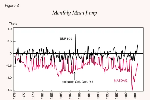
The jump diffusion model outlined above states that the probability distribution of stock returns (measured by log price relatives) is a mixed normal-Poisson process with five parameters. While any or all of these parameters might be affected by margin lend-ing, we assume that the parameters of the simple dif-fusion portion of the model, and , are constant throughout the period of analysis. Margin-related fac-tors enter through their effect on the parameters affect-ing the distribution of jumps. There are three such parameters: the mean frequency of jumps (), the mean size of each jump (), and the volatility, or stan-dard deviation, of each jump (). Because the mean fre-quency is associated with the rate of arrival of new information, a characteristic not clearly related to mar-gin debt, we treat it as a constant. We choose to consid-er the margin-related variables as affecting the mean jump and not the jump volatility. Therefore, we make the mean jump size a linear function of variables that might affect that parameter, including the outstanding amount of margin loans.
We estimate the jump diffusion model using two separate measures of stock returns, the S&P 500 and the NASDAQ Composite. Our theoretical discussion above showed that, in an efficient market, binding lim-its on margin loans would induce leverage-seeking investors to hold riskier stock portfolios. Because the NASDAQ Composite has greater volatility than the S&P 500, we expect that the NASDAQ Composite more closely reflects the index of stocks held by mar-gin-constrained investors; therefore its parameters should be more sensitive to margin lending.
The sample excludes the three months of the final quarter of 1987. The case for including the 1987 break is that it is one of the rare times when margin lending might have made a difference (and, apparently, it does for the S&P 500). The case for excluding it is that the depth of break might have been associated with other causes, such as extreme illiquidity and trading halts, so attributing it to margin lending might be inappro-priate. Including October–December 1987 has little effect on the S&P 500 coefficients but strengthens the margin loan coefficients for the NASDAQ.