Statistical Analysis of Safety Improvements and Integration into Project Design Process

(1)

JOINT TRANSPORTATION

RESEARCH PROGRAM

INDIANA DEPARTMENT OF TRANSPORTATION AND PURDUE UNIVERSITY

Statistical Analysis of Safety

Improvements and Integration into

Project Design Process

Andrew P. Tarko, Mario Romero, Cristhian Lizarazo, Raul Pineda

SPR-4216 • Report Number: FHWA/IN/JTRP-2020/09 • DOI: 10.5703/1288284317121

JOINT TRANSPORTATION

RESEARCH PROGRAM

INDIANA DEPARTMENT OF TRANSPORTATION AND PURDUE UNIVERSITY

Statistical Analysis of Safety

Improvements and Integration into

Project Design Process

Andrew P. Tarko, Mario Romero, Cristhian Lizarazo, Raul Pineda

SPR-4216 • Report Number: FHWA/IN/JTRP-2020/09 • DOI: 10.5703/1288284317121

(2)

RECOMMENDED CITATION

Tarko, A. P., Romero, M., Lizarazo, C., & Pineda, R. (2020).

Statistical analysis of safety improvements and integration

into project design process

(Joint Transportation Research Program Publication No. FHWA/IN/JTRP-2020/09). West

Lafayette, IN: Purdue University. https://doi.org/10.5703/1288284317121

AUTHORS

Andrew P. Tarko, PhD

Professor of Civil Engineering and Director of Center for Road Safety

Lyles School of Civil Engineering

(765) 494-5027

[email protected]

Corresponding Author

Mario Romero, PhD

Research Scientist

Lyles School of Civil Engineering

Purdue University

Cristhian Lizarazo

Raul Pineda

Graduate Research Assistants

Lyles School of Civil Engineering

Purdue University

JOINT TRANSPORTATION RESEARCH PROGRAM

The Joint Transportation Research Program serves as a vehicle for INDOT collaboration with higher education

in-stitutions and industry in Indiana to facilitate innovation that results in continuous improvement in the planning,

design, construction, operation, management and economic efficiency of the Indiana transportation infrastructure.

https://engineering.purdue.edu/JTRP/index_html

Published reports of the Joint Transportation Research Program are available at http://docs.lib.purdue.edu/jtrp/.

NOTICE

The contents of this report reflect the views of the authors, who are responsible for the facts and the accuracy of the

data presented herein. The contents do not necessarily reflect the official views and policies of the Indiana Depart

-ment of Transportation or the Federal Highway Administration. The report does not constitute a standard, specifica

-tion or regula-tion.

(3)

TECHNICAL

REPORT

DOCUMENTATION

PAGE

1. ReportNo.

FHWA/IN/JTRP-2020/09

2. GovernmentAccessionNo. 3. Recipient’sCatalogNo. 4. TitleandSubtitle

StatisticalAnalysisofSafetyImprovementsandIntegrationintoProjectDesign Process

5. ReportDate

April2020

6. PerformingOrganizationCode 7. Author(s)

AndrewP.Tarko,MarioRomero,CristhianLizarazo,andRaulPineda

8. PerformingOrganizationReportNo.

FHWA/IN/JTRP-2020/09

9. PerformingOrganizationNameandAddress

JointTransportationResearchProgram(SPR)

HallforDiscoveryandLearningResearch(DLR),Suite204 207S.MartinJischkeDrive

WestLafayette,IN47907

10. WorkUnitNo. 11. ContractorGrantNo.

SPR-4216

12. SponsoringAgencyNameandAddress

IndianaDepartmentofTransportation StateOfficeBuilding

100NorthSenateAvenue Indianapolis,IN46204

13. TypeofReportandPeriodCovered

FinalReport

14. SponsoringAgencyCode

15. SupplementaryNotes

ConductedincooperationwiththeU.S.DepartmentofTransportation,FederalHighwayAdministration.

16. Abstract

RoadHAT is a tool developed by the Center for Road Safety and implemented for the INDOT safety management practice to help identify both safety needs and relevant road improvements. This study has modified the tool to facilitate a quick and convenient comparison of various design alternatives in the preliminary design stage for scoping small and medium safety-improvement projects. The modified RoadHAT 4D incorporates a statistical estimation of the Crash Reduction Factors based on a before-and-after analysis of multiple treated and control sites with EB correction for the regression-to-mean effect. The new version also includes the updated Safety Performance Functions, revised average costs of crashes, and the comprehensive table of Crash Modification Factors—all updated to reflect current Indiana conditions. The documentation includes updated Guidelines for Roadway Safety Improvements. The improved tool will be implemented at a sequence of workshops for the final end users and preceded with a beta-testing phase involving a small group of INDOT engineers.

17. KeyWords

roadwaysafety,safetymanagement,scopingprojects,crash modificationfactors

18. DistributionStatement

Norestrictions.Thisdocumentisavailablethroughthe NationalTechnicalInformationService,Springfield,VA 22161.

19. SecurityClassif.(ofthisreport)

Unclassified

20. SecurityClassif.(ofthispage)

Unclassified

21. No.ofPages

46including appendices

22. Price

(4)

EXECUTIVE SUMMARY

Introduction

A recent FHWA audit of INDOT’s highway safety programs and procedures called for improvements in current procedures by incorporating safety considerations into the design of all INDOT and local projects. This outcome has prompted the INDOT Bridges and Highway Design Divisions to request the development of improved methods and software to evaluate the traffic safety implications of geometric design decisions. This report presents a study aimed to incorporate a systematic process for integrating the consideration of safety into project scoping and design.

The IHDSM, although calibrated to Indiana conditions in the recent JTRP study, is also suitable for large road projects; however, it requires designers’ significant effort for preparing and entering the input. There is a need for a convenient tool for small and medium projects that can quickly and interactively facilitate a design process through to its completion.

This study was aimed to modify RoadHAT—a tool developed by the Purdue Center for Road Safety (CRS) and implemented for the INDOT safety management to facilitate a quick and convenient comparison of various design alternatives in the preliminary design stage for scoping small and medium safety-improvement projects.

Improvements

N

Multiple design alternatives can be defined with different subsets of safety improvements, be saved, and then compared.

N

Individual design changes of a segment roadway may begin and end anywhere inside a considered segment.

N

Target crashes are introduced for each countermeasure as a percent of crashes at three levels of crash severity to make the analysis versatile and more accurate.

N

The use of target crashes through a percent of all crashes at various severity levels enabled utilization of the existing safety performance functions in economic and before-and-after evaluation.

N

Before-and-after studies of multiple treated and control sites can be facilitated with the improved tool.

N

The statistical significance of safety improvement is esti-mated at the user-selected significance level.

N

A provision for reading the crash location data allows the crash-countermeasure assignments made by the tool to considerably reduce the end-user’s effort.

N

Additional RoadHAT reports have been added for each design alternative, their comparison, and before-and-after studies.

N

The Guidelines for Roadway Safety Improvements, Crash Reduction Factors, and Safety Performance Functions are updated.

Implementation

The RoadHAT 4D is a computer software developed in close collaboration with INDOT users. The project produced a modified RoadHAT tool with embedded documentation to help the end-user. Incorporation of the safety component in the early stage of design and post-construction evaluation will be supported with a sequence of workshops organized by the Business Owner and delivered by the Purdue CRS research team.

After the beta-testing phase, the developed tool will be distributed internally among INDOT units. The Purdue CRS will be involved in the RoadHAT 4D implementation by providing requested help, collecting the users’ feedback, and implementing the recommendations.

(5)

CONTENTS

1. INTRODUCTION . . . 1

2. RESEARCH OBJECTIVES AND SCOPE . . . 1

3. CONCEPT OF REVISED ROADHAT . . . 1

4. PREDICTING SAFETY BENEFITS OF ROAD IMPROVEMENTS . . . 2

4.1 Intersections. . . 2

4.2 Segments . . . 2

5. ESTIMATING CRASH REDUCTION FACTORS . . . 3

5.1 Single Location . . . 3

5.2 Estimating Cash Reduction Factors Using a Control Site . . . 4

5.3 Estimating Crash Reduction Factors Based on Multiple Locations . . . 4

6. UPDATING CRASH REDUCTION FACTORS . . . 5

7. STATISTICAL SIGNIFICANCE OF CRASH REDUCTION. . . 5

8. CLOSURE . . . 6

REFERENCE . . . 6

APPENDICES Appendix A. Updated Safety Performance Functions . . . 7

Appendix B. Revised Crash Costs . . . 7

(6)

LIST OF TABLES

Table Page

(7)

1. INTRODUCTION

The Fixing America’s Surface Transportation (FAST) Act established regulations that require state departments of transportation (DOTs) to analyze and report the resulting safety performance of traffic safety improvement projects that were previously constructed and funded under the Highway Safety Improvement Program (HSIP). The purpose of the federal regulation is to strive for superior decision making in the allocation of highway safety funds to reduce the incidence of crashes resulting in fatalities and severe injuries. Prior to federal fiscal year 2018, state DOT reporting of post construction safety per-formance was largely voluntary. The INDOT Office of Traffic Safety has undertaken comparative ‘‘before/ after’’ safety performance studies of previously com-pleted HSIP projects; however, staff’s current ability to calculate and report statistically significant analyses results is limited.

An appropriate methodology for the evaluation of traffic safety improvement projects is essential to identify the effectiveness of the implemented improve-ments or countermeasures and to quantify its benefits. A recent FHWA audit of INDOT’s highway safety programs and procedures called for improvements in current procedures for incorporating safety considera-tions into the design of all INDOT and local projects. This outcome has prompted the INDOT Bridges and Highway Design Divisions to request development of improved methods and software to evaluate the traffic safety implications of geometric design decisions. This report presents a study aimed to incorporate a syste-matic process for integrating the consideration of safety into project scoping and design applied to existing roads that are selected for safety improvements.

The IHDSM, although calibrated to the Indiana conditions in the recent JTRP study (Tarko et al., 2018) is suitable for large road projects in mind and it requires designers’ significant effort for preparing and entering the input. Yet, it does not support sequential decision-making in the course of design but rather it facilitates a selection of the most promising alternative from several alternatives already designed. Thus, there is a need for a convenient tool for small and medium projects that could facilitate a way to quickly and interactively review design alternatives within a design process up to its completion.

RoadHAT is a tool developed by the Center for Road Safety and successfully implemented to the INDOT safety management practice to help identify both the safety needs and the relevant road improve-ments. It does not allow a quick and convenient comparison of various preliminary design alternatives to facilitate projects scoping.

The applied research study reported in this document modified the existing RoadHAT 3 tool to incorporate its statistical analysis capability as part of post construction performance evaluations, principally Empirical-Bayes (EB) or some other statistical analysis methodology for

various safety improvements on state and local high-ways. This software tool is supposed to support job scoping in the preliminary design stage for small and medium safety-improvement projects and to aid analyz-ing the post-construction performance of safety impro-vement projects. The envisioned new components were embedded in the existing RoadHAT 3 software as RoadHAT 4D. The new version also includes the updated Safety Performance Functions, revised average costs of crashes, and the comprehensive table of Crash Modification Factors updated to reflect the current Indiana conditions.

2. RESEARCH OBJECTIVES AND SCOPE

The scope of work includes analysis of the meth-odologies used in other states by studying the existing publications, research reports, and guidelines. The infor-mation relevant to the project topic will be compiled to determine the best practice process for both the evaluation of traffic safety improvement projects and for estimating the safety implications of geometric design decisions.

A computer application will be developed to incor-porate statistical analysis capability as part of post construction performance evaluations. Performance measures will estimate safety benefits in terms of reduction in number of crashes and long term econo-mic impacts.

The primary research objectives of the proposed project are as follows:

1. Develop a process for integrating road safety considera-tion into project scoping and design.

2. Develop a methodology to evaluate traffic safety impro-vement projects and to update and apply CMFs when multiple countermeasures are proposed.

3. Expand the existing RoadHAT software by integrating the modules developed in Tasks 1 and 2.

3. CONCEPT OF REVISED ROADHAT

The new version—RoadHAT 4D—supports scoping of safety project for existing roads by allowing convenient generation of design alternatives at the level of detail possible before the preliminary design stage. A project alternative is defined with the existing road geometry and traffic control supplemented with the proposed safety countermeasures—changes of the road geometry and traffic control aimed to improve safety. Thus, the default reference alternative is by default do-nothing option. It is not explicitly represented among the alternatives. Instead, all explicitly stated alternatives are compared to the do-nothing alternative by estimat-ing the safety benefits and the project costs.

An alternative is created in Form 5 by adding one or more countermeasures. Each countermeasure is defined with the following elements:

N

_{countermeasure name, possibly including a short} descrip-tion,

(8)

N

_{part of road segment affected by the countermeasures} (start and end points, only for segments),

N

_{crash reduction factors by severity (three levels),}

N

_{percent of crashes that are affected at each severity level}

(target crashes),

N

_{countermeasure}_capital_cost,

N

_change_in_the_maintenance_cost,_and

N

_salvage_value.

The cost components can be entered for every countermeasure if such cost assignments to specific countermeasures are possible. Otherwise, a dummy countermeasure with zero Crash Reduction Factors can be entered together with the capital cost, change in the maintenance cost, and salvage value applicable to mul-tiple countermeasures. More than one dummy counter-measure may be used. The name and description of the dummy countermeasure may state which countermea-sures are included in the cost components.

New countermeasures can be added and existing countermeasures may be copied or deleted. A copied countermeasure may be edited to create a new counter-measure that is not much different from the existing one (for example, different only by affected part of the segment).

Any project alternative can be saved under its own name. Any saved alternative can be read for modifica-tions and saved under its own name or under a differed name to add a new alternative to the already saved ones. Calculated economic components include the follow-ing:

N

_{saved crashes by severity,}

N

_{annualized cost of all crashes saved,}

N

_{annualized cost of the project,}

N

_{annualized net benefit, and}

N

_{B/C ratio.}

Summary of the results of all saved alternatives are available for comparison in Form 6. User selects alter-natives for comparing side by side from a list of all available alternatives. Any alternative already displayed for comparison can be removed. The comparison includes the alternative names, list of alterative names, and the economic components. A report saved by the user includes all the displayed alternatives.

Form 7 is added to facilitate the estimation of the Crash Modification Factors and to evaluate the effectiveness of the safety project in improving safety. The user may enter multiple roads with similar safety project applied to these roads. In addition, the user has an option to include control site in the analysis. A control site is a road without any road changes during the analysis period and similar to the road treated with safety countermeasures. A control site accounts for any overall changes in safety not related to the road improvements and caused by changes in traffic composition, weather, vehicle design, etc.

The effectiveness of the safety improvements are represented with the magnitude of crash reduction and with the statistical significance of this reduction. A statistically significant crash reduction has small

probability that the observed reduction was random and not systematic.

4. PREDICTING SAFETY BENEFITS OF ROAD IMPROVEMENTS

4.1 Intersections

Safety performance function (SPF) for an intersec-tion is:

a~kQc1 1Q

c2

2 (crashes=year)

And the EB estimate of the expected annual number of crashes is:

aEB~

Cz1=a Yz1=(aa)

where:aEB is EB-estimate of the expected number of crashes at the intersection (crashes/year), C is the number of crashes duringYyears, Q1andQ2are the AADTs on the major and minor roads in (1000s veh/h),

k,c1,c2are parameters, andais over-dispersion. The number of saved crashes of certain severity with the countermeasures applied at intersections is:

b~aEBCRF

with Crash Reduction Factor CRF, that represents multiple safety countermeasures applied at the inter-section, being calculated as:

CRF~100: 1{Pn j~1 1{ PTj 100: CRFj 100 where:

CRF5combined Crash Modification Factor repre-senting the effect of all countermeasures applied at the intersection,

PTj5percent of crashes of certain severity are target crashes for countermeasurej,

CRFj5Crash Reduction Factor of countermeasurej.

4.2 Segments

The total number of crashes on the segment C and the segment length isL.A safety performance function (SPF) for a segment is:

a~kLb_Qc

where: a is the expected number of crashes on the segments (crashes/year),Lis the segment length (mi),Q

is the AADT in (1000s veh/h),k,b,care parameters, and

ais over-dispersion.

The total number of crashes on the segment C. Let the segment be divided into sub-segments of lengths:

l1,l2, andlmwith crash counts:c1,c2, andcm. The SPF-based expected number of crashes on any sub-segmentiis:

ai~ li L kL b_Qc_~_kl iLb {1_Qc

(9)

and theinitialEB-based expected number of crashesaBi on any sub-segment iis:

aBi~

ciz1=a 1z1=(aai)

Whereci5is the number of crashes on sub-segmenti. The EB-based total number of crashes on the seg-ment is:

aEB~

Cz1=a

1z1=(aa)

The adjustedEB-based expected number of crashes

aEBion any sub-segmentiis:

aEBi~aEBPaBi iaBi CRFi~100: 1{Pj ~ni j~1 1{ PTi,j 100 : CRFi,j 100 where:

CRFi5 combined Crash Modification Factor repre-senting the effect of all countermeasures applied on sub-segment i,

PTi,j5 percent of crashes of certain severity on sub-segment i that are target crashes for countermea-surej,

CRFi,j5Crash Reduction Factor of countermeasure

j applied on segmenti.

The number of crashes of certain severity saved on the entire segment is:

b~Pm_i_~₁aEBiCRFi

When the distribution of crashes among sub-segments is not known, the simplest approximation is based on the assumption that the crashes are distrib-uted in proportion of the sub-segment lengths. Thus:

b~ m_i_~₁ li

L aEBCRFi

P

5. ESTIMATING CRASH REDUCTION FACTORS The effectiveness of a safety project should be reevaluated after its implementation to provide feed-back to the safety management process. This feedfeed-back helps improve future decision about specific safety improvement and prediction of their effectiveness. The post implementation study uses crash data collected before and after the project is implemented. Although the recommended periods before and after the imple-mentation are three years for each period, longer periods increase the confidence of the results and should be considered. In all cases, the periods should be multiples of full years to eliminate the undesirable effect of seasonal variations of crashes. Other data needed for a post-implementation study include actual project

costs, annual maintenance costs, traffic growth rate, and average daily traffic volumes.

The outcome from the post implementation study includes the following: updated crash reduction factor (CRF) and the measures of economic effectiveness (B/C ratio, net annual benefits, and present worth of total net benefit). The method of analysis is the same as presented in chapter 6. The difference is the updated inputs. The following sections present the most difficult component of post implementation study—estimating and updating crash reduction factors. The method is introduced gradually by consideration of a single site. Then, a control site is added to account for safety factors other than the safety project. Next, a case of multiple treated and control sites is presented. Finally, a method of combining the new crash reduction factors with the existing one is shown.

5.1 Single Location

Crash Reduction Factors are used in calculating benefits provided by a safety project as the percent of original crashes reduced by the implementation of the safety project. The crash reduction factor for the project is calculated using crash reported before and after implementing the safety project. Expected crash frequency a0A in the period after implementation of a safety project, had the safety project not been imple-mented, is calculated to account for the ‘‘regression-to-mean effect’’ and for the change in traffic volume. The available safety performance functions estimate the frequency of all crashes at different levels of severity while some CRFs are applicable only to, so-called, target crashes to account for the fact that a considered countermeasure affects only some type of crashes. For example, installing a median barrier reduces head-on collisihead-ons. This is accounted for in the calculatihead-on with the percent of target crashes (PT) that is used to reduce the crash frequencies estimated with safety performance functions to the frequency of target crashes.

The crash reduction factor for the implemented safety project CRF2 and its standard deviation are calculated. Crash reduction factors are estimated for all crashes, incapacitating injury and fatal (NI) crashes, non-incapacitating injuries (NI) crashes, and property damage only (PD) crashes separately.

a0A~ 1 DzCB 100 D:PT:aB zYB : aA aB a1A~ CA YA var a0A~ 1 DzCB 100 D:PT:aBzYB 2: aA aB 2

(10)

var a1A~ CA Y2 A CRF2~100 1{ a1A a0A SD2~100 ffiffiffiffiffiffiffiffiffiffiffiffiffiffiffiffiffiffiffiffiffiffiffiffiffiffiffiffiffiffiffiffiffiffiffi var a1A a2 0A za 2 A a0A a4 0A s where:

a0A5 best estimate of the target crash frequency in the period after the implementation of safety project, had the safety project not been implemented, this estimate is the combination of crash counts and the result obtained with a safety performance function,

a1A5target crash frequency estimate for the period after the project implementation, this estimate is based on crashes that occurred at the improved site,

aA5 crash frequency (total of target and non-target crashes) calculated with a safety performance function and for traffic representing the after-implementation period,

aB5crash frequency (total of target and non-target crashes) calculated with a safety performance function and for traffic representing the before-implementation period,

CA5number of reported target crashes (affected by the countermeasure) that occurred during the period after the implementation of safety project,

CB5number of target crashes that occurred during the period before the implementation of safety project,

CRF25crash reduction factor estimate, in percent,

D5 over-dispersion parameter associated with the safety performance function used to calculateaAandaB

PT5 percent of crashes that are affected by the countermeasure (target crashes), in percent,

SD25 standard deviation of the crash reduction factor estimate for the implemented safety project, in percent,

var a0A5variance ofa0A estimate,

var a1A5variance ofa1A estimate,

YB5 number of before-implementation years with crash data, and

YA5 number of after-implementation years with crash data.

5.2 Estimating Cash Reduction Factors Using a Control Site

In order to account for unknown factors that may cause a change in the number of crashes after imple-mentation of the safety project, crash reduction factors are calculated using a control group, which consists of locations that have characteristics similar to locations where the safety project is implemented, but at these locations the safety project is not implemented. The expected number of crashes per year in the period after implementation of the safety project assuming no road

improvement,a0A, and the number of crashes per year during the period after the implementation of the safety project, a1A, are calculated for the treated sites. The

0 0

same equations are used to calculatea₀_Aanda₁_Afor the control site. The before and after periods for the control site should match the corresponding period for the treated site. A, so-called, crash reductionhis the ratio ofa1Aanda0A:

h~a1A

a0A The variance ofhestimate is:

varh~ 1 a0A 2 :_{var a}₁_Az a1A a2 0A 2 : _{var a}₀_A

The corresponding ratio h’ is calculated for the

0 0

control sites using a₁_A and. a₀_A Its variance of h’ estimate for the control site is calculated with the same equation of the variance ofhestimate.

The crash reduction factorCRF2, which includes the adjustment for safety factors other than the safety project and the change in traffic volume, is estimated as follows:

CRF2~100 1{

h

h’

The variance of the CRF2 estimate is calculated as follows: SD2~100 ffiffiffiffiffiffiffiffiffiffiffiffiffiffiffiffiffiffiffiffiffiffiffiffiffiffiffiffiffiffiffiffiffiffiffiffiffiffiffiffiffiffiffiffiffiffiffiffiffiffiffiffiffiffiffiffiffiffiffi 1 h’ 2 :_var_hz h h’2 2 :_var_h_’ s where:

h5 crash reduction at the location with treated group,

var h5variance ofhestimate,

0

h5 crash reduction at the location with control group,

varh’5variance ofh0 estimate,

CRF25 crash reduction factor after implementing the safety project, in percent, and

SD25 standard deviation of the crash reduction factor for the implemented safety project, in percent.

5.3 Estimating Crash Reduction Factors Based on Multiple Locations

Crash reduction factors are key inputs to estimating safety benefits. They should be as accurate as possible. One of the methods of improving accuracy and precision of crash reduction factors estimates is using multiple treated and control sites. It is required that all the treated sites included in the analysis undergo the same type of improvement. The control group of sites where no improvements are implemented should be in the same geographical area as the treated sites. The average before periods for the treated and control sites 4 Joint Transportation Research Program Technical Report FHWA/IN/JTRP-2020/09

(11)

should be the similar. The same is required for the average after period.

Modernization of different sites takes place in different years. To preserve the adjusting capabilities of the control sites, each of the treated sites should have at least one control site of the same type and similar characteristics, if possible. The treated and correspond-ing control sites should be similar and have the same before periods and the same after periods.

The idea of analyzing multiple sites is to aggregate the treated sites and the control sites into two single entities. This aggregation allows using the equations already developed for single sites. The first step is to estimate the annual number of crashes and the variance of this estimate for each treated and control site for the before and after periods using equation presented above. Then, the annual frequencies and their variances are summed up to obtain singles values representing the treated group of sites. The same aggregation operation is done for the control group. After this aggregation, the estimation method applicable to a single treated site with a single control site presented above is used.

a1A~P i aAi var a1A~P i var a1Ai a0A~P i a0Ai var a0A~ i var a0Ai P

The above summation over multiple sites is done for crashes at each of the three severity levels, (incapacitating IN, non-incapacitating NI, and property damage only PD) or for all crashes regardless of the severity. Thus, the obtained estimates: a1A, var a1A, a0A, var a0A, apply to each of the three severity levels or two all crashes. 6. UPDATING CRASH REDUCTION FACTORS

This section describes the calculations of the crash reduction factor applicable to crash counts at three severity levels and to all crash count as well. The calculated values are then combined with the existing crash reduction factors (if available) to obtain the best estimates of the crash reduction factors.

Let CRF1 stand for the old crash reduction factor taken from Appendix C, whileCRF2is calculated. The updated crash reduction factor, CRF, is calculated using theCRF1andCRF2estimates and their standard deviationsSD1andSD2respectively:

CRF~SD 2 1:CRF2zSD22:CRF1 SD2 1zSD22 where:

CRF5updated crash reduction factor, percent,

SD15 standard deviation of the old crash reduc-tion factor estimate (assume 25% if not available), in percent, and

SD25standard deviation of the new crash reduction factor estimate for the implemented safety project, in percent.

The standard deviation of the updated crash reduc-tion factor is calculated with standard deviareduc-tions SD1 andSD2, as follows: SD~ ffiffiffiffiffiffiffiffiffiffiffiffiffiffiffiffiffiffiffiffiffiffiffiffiffiffiffiffiffiffiffiffiffiffiffiffiffiffiffiffiffiffi SD4 2:SD 2 1zSD41:SD 2 2 SD2 1zSD22 s

where:SD1andSD2are the standard deviations of the old and updated crash reduction factors. The calculated

SD becomes SD1 when the crash reduction factor is updated again.

7. STATISTICAL SIGNIFICANCE OF CRASH REDUCTION

The agency may want to test the statistical significance of the effectiveness of a safety project to determine whether the reduction in crashes is large enough to reject the possibility that the reduc-tion was caused solely by random fluctuareduc-tions of crashes. A one-tail test is used to decide if the obtained crash reduction factor is significantly larger than zero. The estimate of the crash reduction factor is assumed to be normally distributed. The recom-mended significance levels are 1%, 5%, and 10%. The default value is 10%.

The significance for the safety change is per-formed at a user selected significance level. The choice of significance level depends on the project size (cost). A significance level of 5% can be used for large and expensive projects, while 10% may be used for small projects. The 10% significance level is considered typical in post-implementation studies.

Table 7.1 helps determine whether the reduction in crashes is significant at 1%, 5%, 10%significance level. If normalized value Z=CRF/SD is larger than the critical value Zc, then the safety improve-ment is statistically significant at the selected level of significance.

TABLE 7.1

Critical ValueZc

Significance Level (%) Critical ValueZc

1 5 10 2.33 1.65 1.28

(12)

8. CLOSURE

The project has produced a modified RoadHAT 4D tool with companion user’s manual. The user manual is embedded in the installation package and available via a Help link included in each form. The manuals first page provides links to all parts, elements, and terms of the tool. A revised version of the Guidelines are also included to introduce and help interpret of the elements of the safety management concepts.

Incorporation of the safety component in the early stage of design should increase the effectiveness of the project in reducing the frequency and severity of crashes. The second component of the project: post-construction evaluation, should have two-fold benefit. 1. The tool confirms which projects were successful and why.

This feedback may help refocus future investments on

projects that have a higher chance of being successful, thus leading to an additional improvement of road safety—the ultimate goal of all safety-related efforts. 2. The tool includes the components of the design

metho-dology that should be tuned to produce better results. Specifically, two important improvements that need to be updated as needed are: (1) crash Modification Factors of road improvements, (2) costs of various road improve-ments.

REFERENCE

Tarko, A. P., Romero, M., Hall, T., & Sultana, A. (2018). Updating the crash modification factors and calibrating the IHSDM for Indiana (Joint Transportation Research Pro-gram Publication No. FHWA/IN/JTRP-2018/03). West Lafayette, IN: Purdue University. https://doi.org/10.5703/ 1288284316646

(13)

APPENDICES

Appendix A. Updated Safety Performance Functions

Appendix B. Revised Crash Costs

Appendix C. Updated Crash Modification Factors

(14)

APPENDIX

A. UPDATED SAFETY

PERFORMANCE FUNCTIONS

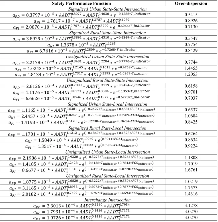
Table A.1 State Intersections

Safety Performance

Function

Over-dispersion

Signalized Urban State-State Intersection

𝑎

=

8.3797

∗

10 ∗

𝐴𝐴𝐷𝑇

.

∗

𝐴𝐴𝐷𝑇

.

∗

𝑒

. ∗ _

0.5415

𝑎

=

1.7617

∗

10 ∗

𝐴𝐴𝐷𝑇

.

∗

𝐴𝐴𝐷𝑇

.

0.8926

𝑎

=

2.8870

∗

10 ∗

𝐴𝐴𝐷𝑇

.

∗

𝐴𝐴𝐷𝑇

.

∗

𝑒

. ∗ _

_0.7130

Signalized Rural State-State Intersection

𝑎

=

3.8929

∗

10 ∗

𝐴𝐴𝐷𝑇

.

∗

𝐴𝐴𝐷𝑇

.

∗

𝑒

. ∗ _

0.5547

𝑎

=

1.3378

∗

10 ∗

𝐴𝐴𝐷𝑇

.

_0.7754

𝑎

=

6.7616

∗

10 ∗

𝐴𝐴𝐷𝑇

.

_∗

_𝑒

. ∗ _

_0.8429

Unsignalized Urban State-State Intersection

𝑎

=

2.2178

∗

10 ∗

𝐴𝐴𝐷𝑇

.

_∗

_{𝐴𝐴𝐷𝑇}

.

_∗

_𝑒

. ∗ _

_0.7744

𝑎

=

1.0243

∗

10 ∗

𝐴𝐴𝐷𝑇

.

_∗

_{𝐴𝐴𝐷𝑇}

.

_∗

_𝑒

. ∗

_1.4455

𝑎

=

4.8134

∗

10 ∗

𝐴𝐴𝐷𝑇

.

∗

𝐴𝐴𝐷𝑇

.

∗

𝑒

. ∗

1.2053

Unsignalized Rural State-State Intersection

𝑎

=

2.6126

∗

10 ∗

𝐴𝐴𝐷𝑇

.

∗

𝐴𝐴𝐷𝑇

.

∗

𝑒

. ∗ _

0.6158

𝑎

=

1.1176

∗

10 ∗

𝐴𝐴𝐷𝑇

.

∗

𝐴𝐴𝐷𝑇

.

∗

𝑒

. ∗ _

0.9701

𝑎

=

6.6626

∗

10 ∗

𝐴𝐴𝐷𝑇

.

∗

𝐴𝐴𝐷𝑇

.

∗

𝑒

. ∗ _

0.7037

Signalized Urban State-Local Intersection

𝑎

=

1.1165

∗

10 ∗

𝐴𝐴𝐷𝑇

.

∗

𝑒

( . ∗ . ∗ )

_0.6537

𝑎

=

2.4457

∗

10 ∗

𝐴𝐴𝐷𝑇

.

∗

𝑒

( . ∗ . ∗ )

1.0684

𝑎

=

1.4198

∗

10 ∗

𝐴𝐴𝐷𝑇

.

∗

𝑒

( . ∗ . ∗ )

0.8425

Signalized Rural State-Local Intersection

𝑎

=

1.1701

∗

10 ∗

𝐴𝐴𝐷𝑇

.

∗

𝑒

( . ∗ . ∗ )

0.6264

𝑎

=

1.5849

∗

10 ∗

𝐴𝐴𝐷𝑇

.

_∗

_𝑒

( . ∗ )

_0.8634

𝑎

=

1.3517

∗

10 ∗

𝐴𝐴𝐷𝑇

.

∗

𝑒

( . ∗ )

0.9224

Unsignalized Urban State-Local

Intersection

𝑎

=

2.1986

∗

10 ∗

𝐴𝐴𝐷𝑇

.

∗

𝑒

( . ∗ . ∗ )

1.1808

𝑎

=

1.4185

∗

10 ∗

𝐴𝐴𝐷𝑇

.

∗

𝑒

( . ∗ . ∗ )

_1.7019

𝑎

=

8.6677

∗

10 ∗

𝐴𝐴𝐷𝑇

.

∗

𝑒

( . ∗ . ∗ )

1.6761

Unsignalized Rural State-Local

Intersection

𝑎

=

1.8775

∗

10 ∗

𝐴𝐴𝐷𝑇

.

∗

𝑒

( . ∗ . ∗ )

1.0219

𝑎

=

3.1165

∗

10 ∗

𝐴𝐴𝐷𝑇

.

∗

𝑒

( . ∗ . ∗ )

1.7573

𝑎

=

2.0182

∗

10 ∗

𝐴𝐴𝐷𝑇

.

_∗

_𝑒

( . ∗ . ∗ )

_1.4316

Interchange

Intersection

𝑎

=

3.3013

∗

10 ∗

𝐴𝐴𝐷𝑇

.

∗

𝐴𝐴𝐷𝑇

.

3.1278

𝑎

=

1.7931

∗

10 ∗

𝐴𝐴𝐷𝑇

.

∗

𝐴𝐴𝐷𝑇

.

3.0270

𝑎

=

1.0726

∗

10 ∗

𝐴𝐴𝐷𝑇

.

∗

𝐴𝐴𝐷𝑇

.

3.0270

Where:

𝑎

=

annual number of property-damage-only (PD) crashes

𝑎

=

annual number of non-incapacitating or possible (NI) crashes

(15)

𝑎

=

annual number of fatal or incapacitating (FI) crashes

𝐴𝐴𝐷𝑇

= Annual Average Daily Traffic (AADT) along the major road

𝐴𝐴𝐷𝑇

= Annual Average Daily Traffic (AADT) along the minor road

𝑇

= binary indicator showing the presence of a T-intersection (1 if present, 0 otherwise)

𝑈𝑟𝑏𝑎𝑛

= binary indicator showing the presence of a urban area (1 if present, 0 otherwise)

𝐹𝐶3

= binary indicator showing the presence of a principal arterial (1 if present, 0 otherwise)

𝐹𝐶4

= binary indicator showing the presence of a minor arterial (1 if present, 0 otherwise)

𝐹𝐶5

= binary indicator showing the presence of a major collector (1 if present, 0 otherwise)

𝐹𝐶6

= binary indicator showing the presence of a minor collector (1 if present, 0 otherwise)

𝐹𝐶34

= binary indicator showing the presence of a principal arterial or a minor arterial (1 if

present, 0 otherwise)

𝐹𝐶56

= binary indicator showing the presence of a major collector or a minor collector (1 if

present, 0 otherwise)

(16)

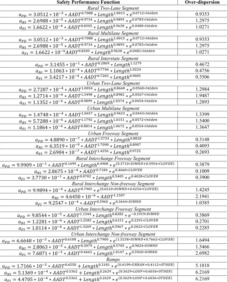
Table A.2 State Segments SPF

Safety Performance

Function

Over-dispersion

Rural

Two-Lane Segment

𝑎

=

3.0512

∗

10 ∗

𝐴𝐴𝐷𝑇

.

∗

𝐿𝑒𝑛𝑔𝑡ℎ

.

∗

𝑒

. ∗

0.9353

𝑎

=

2.6988

∗

10 ∗

𝐴𝐴𝐷𝑇

.

_∗

_{𝐿𝑒𝑛𝑔𝑡ℎ}

.

_∗

_𝑒

. ∗

_1.2975

𝑎

=

1.6622

∗

10 ∗

𝐴𝐴𝐷𝑇

.

_∗

_{𝐿𝑒𝑛𝑔𝑡ℎ}

.

_∗

_𝑒

. ∗

_1.0271

Rural

Multilane Segment

𝑎

=

3.0512

∗

10 ∗

𝐴𝐴𝐷𝑇

.

∗

𝐿𝑒𝑛𝑔𝑡ℎ

.

∗

𝑒

. ∗

0.9353

𝑎

=

2.6988

∗

10 ∗

𝐴𝐴𝐷𝑇

.

∗

𝐿𝑒𝑛𝑔𝑡ℎ

.

∗

𝑒

. ∗

1.2975

𝑎

=

1.6622

∗

10 𝐴𝐴𝐷𝑇

.

∗

𝐿𝑒𝑛𝑔𝑡ℎ

.

∗

𝑒

. ∗

1.0271

Rural

Interstate

Segment

𝑎

=

3.1455

∗

10 ∗

𝐴𝐴𝐷𝑇

.

∗

𝐿𝑒𝑛𝑔𝑡ℎ

.

0.4672

𝑎

=

1.1063

∗

10 ∗

𝐴𝐴𝐷𝑇

.

_∗

_{𝐿𝑒𝑛𝑔𝑡ℎ}

.

_0.4756

𝑎

=

3.4217

∗

10 ∗

𝐴𝐴𝐷𝑇

.

∗

𝐿𝑒𝑛𝑔𝑡ℎ

.

0.3506

Urban Two-Lane Segment

𝑎

=

2.7287

∗

10 ∗

𝐴𝐴𝐷𝑇

.

∗

𝐿𝑒𝑛𝑔𝑡ℎ

.

∗

𝑒

. ∗

1.2984

𝑎

=

1.2714

∗

10 ∗

𝐴𝐴𝐷𝑇

.

_∗

_{𝐿𝑒𝑛𝑔𝑡ℎ}

.

_∗

_𝑒

. ∗

_1.9487

𝑎

=

1.1352

∗

10 ∗

𝐴𝐴𝐷𝑇

.

_∗

_{𝐿𝑒𝑛𝑔𝑡ℎ}

.

_∗

_𝑒

. ∗

_1.2893

Urban Multilane Segment

𝑎

=

1.4748

∗

10 ∗

𝐴𝐴𝐷𝑇

.

∗

𝐿𝑒𝑛𝑔𝑡ℎ

.

∗

𝑒

. ∗

1.3399

𝑎

=

5.7288

∗

10 ∗

𝐴𝐴𝐷𝑇

.

∗

𝐿𝑒𝑛𝑔𝑡ℎ

.

∗

𝑒

. ∗

1.5400

𝑎

=

1.1864

∗

10 ∗

𝐴𝐴𝐷𝑇

.

∗

𝐿𝑒𝑛𝑔𝑡ℎ

.

∗

𝑒

. ∗

1.3647

Urban Freeway Segment

𝑎

=

4.8890

∗

10 ∗

𝐴𝐴𝐷𝑇

.

_∗

_{𝐿𝑒𝑛𝑔𝑡ℎ}

.

_0.3148

𝑎

=

6.3519

∗

10 ∗

𝐴𝐴𝐷𝑇

.

∗

𝐿𝑒𝑛𝑔𝑡ℎ

.

0.4093

𝑎

=

2.6904

∗

10 ∗

𝐴𝐴𝐷𝑇

.

_∗

_{𝐿𝑒𝑛𝑔𝑡ℎ}

.

_0.2693

Rural

Interchange Freeway

Segment

𝑎

=

9.9909

∗

10 ∗

𝐴𝐴𝐷𝑇

.

∗

𝐿𝑒𝑛𝑔𝑡ℎ

.

∗

𝑒

( . ∗ . ∗ )

0.3879

𝑎

=

2.8675

∗

10 ∗

𝐴𝐴𝐷𝑇

.

∗

𝑒

. ∗

0.1009

𝑎

=

3.7730

∗

10 ∗

𝐴𝐴𝐷𝑇

.

_∗

_{𝐿𝑒𝑛𝑔𝑡ℎ}

.

_∗

_𝑒

. ∗

_0.3900

Rural

Interchange

Non-freeway Segment

𝑎

=

9.9894

∗

10 ∗

𝐴𝐴𝐷𝑇

.

∗

𝑒

( . ∗ . ∗ )

1.4245

𝑎

=

4.6450

∗

10 ∗

𝐴𝐴𝐷𝑇

.

2.1941

𝑎

=

9.2547

∗

10 ∗

𝐴𝐴𝐷𝑇

.

_∗

_𝑒

. ∗

_1.0385

Urban Interchange Freeway Segment

𝑎

=

9.8544

∗

10 ∗

𝐴𝐴𝐷𝑇

.

∗

𝐿𝑒𝑛𝑔𝑡ℎ

.

∗

𝑒

. ∗

0.3869

𝑎

=

1.2281

∗

10 ∗

𝐴𝐴𝐷𝑇

.

∗

𝐿𝑒𝑛𝑔𝑡ℎ

.

∗

𝑒

. ∗

0.2701

𝑎

=

1.0114

∗

10 ∗

𝐴𝐴𝐷𝑇

.

_∗

_{𝐿𝑒𝑛𝑔𝑡ℎ}

.

_∗

_𝑒

. ∗

_0.2285

Urban Interchange Non-freeway Segment

𝑎

=

6.6648

∗

10 ∗

𝐴𝐴𝐷𝑇

.

∗

𝐿𝑒𝑛𝑔𝑡ℎ

.

∗

𝑒

( . ∗ . ∗ )

1.6494

𝑎

=

2.8063

∗

10 ∗

𝐴𝐴𝐷𝑇

.

∗

𝐿𝑒𝑛𝑔𝑡ℎ

.

∗

𝑒

. ∗

1.5466

𝑎

=

7.6871

∗

10 ∗

𝐴𝐴𝐷𝑇

.

_∗

_{𝐿𝑒𝑛𝑔𝑡ℎ}

.

_∗

_𝑒

. ∗

_2.6982

Ramps

𝑎

=

1.7166

∗

10 ∗

𝐴𝐴𝐷𝑇

.

+

𝐿𝑒𝑛𝑔𝑡ℎ

.

∗

𝑒

( . ∗ . ∗ )

5.1818

𝑎

=

5.1369

∗

10 ∗

𝐴𝐴𝐷𝑇

.

+

𝐿𝑒𝑛𝑔𝑡ℎ

.

∗

𝑒

( . ∗ . ∗ )

6.2169

𝑎

=

4.4705

∗

10 ∗

𝐴𝐴𝐷𝑇

.

+

𝐿𝑒𝑛𝑔𝑡ℎ

.

∗

𝑒

( . ∗ . ∗ )

6.2169

A-3

(17)

Where:

𝑎

=

annual number of fatal and incapacitating (FI) crashes

𝑎

=

annual number of non-incapacitating or possible (NI) crashes

𝑎

=

annual number of property damage only (PD) crashes

AADT = Annual Average

Daily

Traffic (AADT) along the segment

Length

= Length of the segment

in mile

Intden = no of minor intersection/segment length in

mile

CLOVER

= indicator variable for cloverleaf interchange (1 if present, 0 otherwise)

DIMND =indicator variable

for diamond interchange (1 if present, 0 otherwise)

DIRECT = indicator variable for directional

interchange (1 if present, 0 otherwise)

JUG = indicator variable for jug-handle

interchange

(1 if present, 0 otherwise)

TRUMPO = indicator variable for trumpet and other interchange (1 if present,

0 otherwise)

Diag

= diagonal ramp

OTHER

= other ramp (1 if other ramp type, 0 otherwise)

LOOP

= loop ramp (1 if a loop ramp, 0 otherwise)

URBAN

= urban indicator (1 if urban area, 0 otherwise).

(18)

APPENDIX B. REVISED

CRASH

COSTS

The average costs of crashes were estimated by calculating the individual crash cost considering the

number of people killed/injured and the number of vehicles damaged. The averages of these costs then

were obtained for the different types of segments/intersections/ramps.

The average cost of one fatality (K) is $10,562,000 and one incapacitating injury (A) is $1,155,000; the

cost for a non-incapacitating (B) injury is considered as $318,000 and the cost of a possible injury (C) is

considered as $147,000. On the other hand, for property damage only crashes (O), the average cost of a

no injury is $11,900 and the cost per vehicle is $4,400 (source: National Safety Council, 2017,

https://injuryfacts.nsc.org/all-injuries/costs/guide-to-calculating-costs/data-details/

The cost of a crash was calculated in the following way:

1. Calculate the cost of each crash

𝐶

=

$4,400

· 𝐷𝑉

+

𝐶𝑂

· $11,900

+

$147,000

· 𝐶𝑃

+

$318,000

· 𝐵𝑃

+

$1,155,000

· 𝐴𝑃

+

$10,562,000

· 𝐾𝑃

where:

𝐶

= crash cost ($),

𝐾𝑃

= number of fatalities (persons),

𝐴𝑃

= number of incapacitating injuries (persons),

𝐵𝑃

= number non-incapacitating injuries (persons),

𝐶𝑃

= number of possible injuries (person),

𝐶𝑂

= number of no injuries (person),

𝐷𝑉

= number of damaged vehicles.

2. Group crashes by road type and crash severity (FI, NI, PD)

3. Calculate the average cost of crash in each group

gr

∑

∈

𝐶

=

𝑁

where:

𝐶

= average cost of crash in crash group

gr

,

𝐼

= indices of crashes that belong to crash group

gr

,

𝐶

= cost of crash

i

calculated in step 1,

𝑁

= number of crashes in group

gr

.

(19)

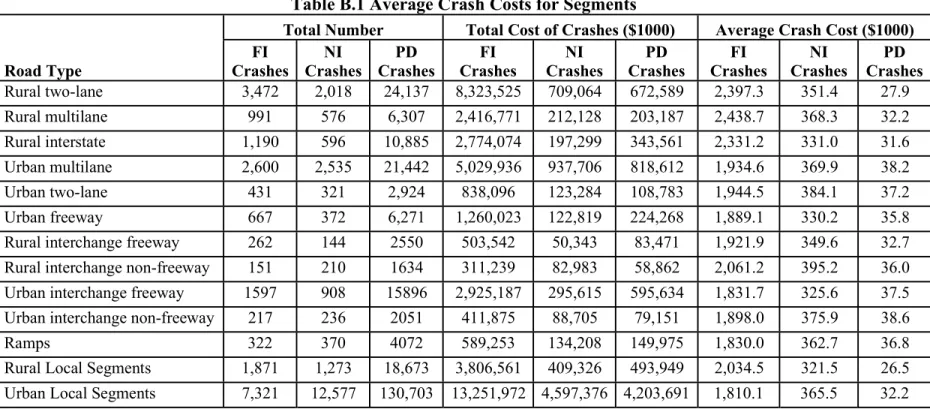
Table

B.1 Average Crash Costs for Segments

Road Type

Total Number

Total

Cost of Crashes ($1000)

Average Crash Cost

($1000)

FI

Crashes

NI

Crashes

PD

Crashes

FI

Crashes

NI

Crashes

PD

Crashes

FI

Crashes

NI

Crashes

PD

Crashes

Rural two-lane

3,472

2,018

24,137

8,323,525

709,064

672,589

2,397.3

351.4

27.9 Rural multilane

991

576 6,307

2,416,771

212,128

203,187

2,438.7

368.3

32.2 Rural interstate

1,190

596 10,885

2,774,074

197,299

343,561

2,331.2

331.0

31.6 Urban multilane

2,600

2,535

21,442

5,029,936

937,706

818,612

1,934.6

369.9

38.2 Urban two-lane

431

321 2,924

838,096

123,284

108,783

1,944.5

384.1

37.2 Urban freeway

667

372 6,271

1,260,023

122,819

224,268

1,889.1

330.2

35.8 Rural interchange freeway

262

144 2550

503,542

50,343

83,471

1,921.9

349.6

32.7 Rural interchange non-freeway

151

210 1634

311,239

82,983

58,862

2,061.2

395.2

36.0 Urban interchange freeway

1597

908 15896

2,925,187

295,615

595,634

1,831.7

325.6

37.5 Urban interchange non-freeway

217

236 2051

411,875

88,705

79,151

1,898.0

375.9

38.6 Ramps

322

370 4072

589,253

134,208

149,975

1,830.0

362.7

36.8 Rural Local Segments

1,871

1,273

18,673

3,806,561

409,326

493,949

2,034.5

321.5

26.5 Urban Local Segments

7,321

12,577

130,703

13,251,972

4,597,376

4,203,691

1,810.1

365.5

32.2

Note: The average crash costs increased considerablyin 2016 when the comprehensive costs replaced the economic loss used in thepreviousyears. Thecomprehensiveunit costs are updated by NHTSA on regular basis and they tend togrow atrather high rate.Another source of the average crash costs increase was the 2016modification of the Incapacitating Injury criterion. This effect waslimited.

(20)

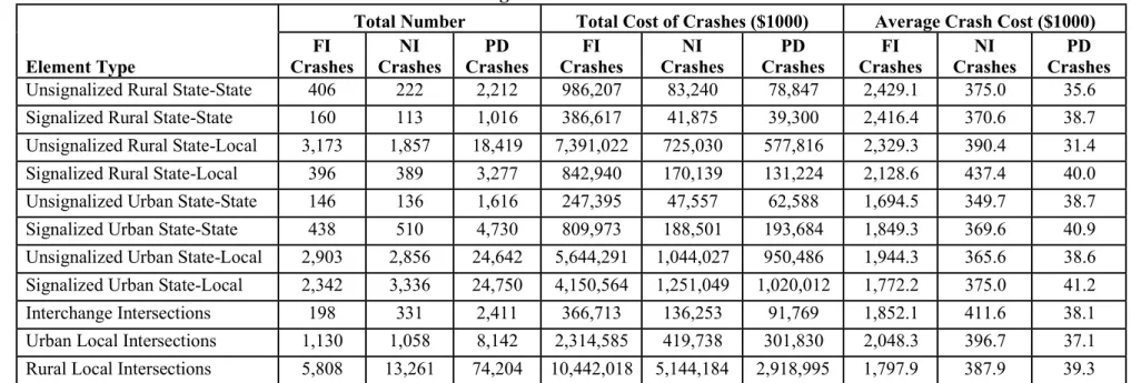
Table

B.2 Average Crash Costs for Intersections

Element Type

Total Number

Total Cost of Crashes ($1000)

Average Crash Cost ($1000)

FI

Crashes

NI

Crashes

PD

Crashes

FI

Crashes

NI

Crashes

PD

Crashes

FI

Crashes

NI

Crashes

PD

Crashes

Unsignalized Rural State-State

406

222 2,212

986,207

83,240

78,847

2,429.1

375.0

35.6 Signalized Rural State-State

160

113 1,016

386,617

41,875

39,300

2,416.4

370.6

38.7 Unsignalized Rural State-Local

3,173

1,857

18,419

7,391,022

725,030

577,816

2,329.3

390.4

31.4 Signalized Rural State-Local

396

389 3,277

842,940

170,139

131,224

2,128.6

437.4

40.0 Unsignalized Urban State-State

146

136 1,616

247,395

47,557

62,588

1,694.5

349.7

38.7 Signalized Urban State-State

438

510 4,730

809,973

188,501

193,684

1,849.3

369.6

40.9 Unsignalized Urban State-Local

2,903

2,856

24,642

5,644,291

1,044,027

950,486

1,944.3

365.6

38.6 Signalized Urban State-Local

2,342

3,336

24,750

4,150,564

1,251,049

1,020,012

1,772.2

375.0

41.2 Interchange Intersections

198

331 2,411

366,713

136,253

91,769

1,852.1

411.6

38.1 Urban Local Intersections

1,130

1,058

8,142

2,314,585

419,738

301,830

2,048.3

396.7

37.1 Rural Local Intersections

5,808

13,261

74,204

10,442,018

5,144,184

2,918,995

1,797.9

387.9

39.3

Note: The average crash costs increased considerablyin 2016 when the comprehensive costs replaced the economic loss used in thepreviousyears. Thecomprehensiveunit costs are updated by NHTSA on regular basis and they tend to grow at ratherhigh rate. Another source of theaverage crash costs increase was the 2016 modificationofthe Incapacitating Injury criterion.This effect waslimited.

(21)

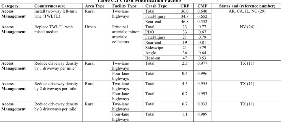
Table

C.1 Crash Modification Factors

Category Countermeasure Area Type Facility Type CrashType CRF CMF States and (reference number)

Access Install two-way left-turn Rural Two-lane Total 36.0 0.640 AR, CA, IL, NC (29)

Management lane (TWLTL) highways Fatal/Injury 34.8 0.652

Rear-end 46.8 0.532

Access Replace TWLTLwith Urban Principal Total 23 0.77 NV (24)

Management raised median arterials; minor PDO 33 0.67

arterials; Fatal/Injury 21 0.79 collectors _Rear-end ₁₉ _0.81 Sideswipe 21 0.79

Angle 36 0.64

Head-on 47 0.53

Access Reduce driveway density Rural Two-lane Total 2.3 0.977 TX (11)

Management by 1 driveway per mile1 _highways

Four-lane Total 0.4 0.996 highways

Access

Management Reduce driveway density by 2 driveways per mile1 Rural Two-lane_highways Total 4.5 0.955 TX (11)

Access Reduce driveway density Rural Two-lane Total 6.7 0.933 TX (11)

Management by 3 driveways per mile1 _highways

APPENDIX C. UPDATED CRASH MODIFICATION

FACTORS

The following table presents the CRFs/CMFs for safety countermeasures that were identified as being the most suitable for Indiana

based on the criteria presented in the Joint Transportation Research Program technical report, “Updating the Crash Modification Factors

and Calibrating the

IHSDM for Indiana”

(Tarko

et

al., 2018). The

table contains 82 safety countermeasures spanning 16 different

categories. For each countermeasure, the

applicable

areas type (urban and/or rural), facility type, and CRF/CMF

values for various crash

types and severities are presented. Finally, the state(s) where each study was conducted and the corresponding reference are provided in

the table.

(22)

Access Reduce driveway density Urban Principal Total 4.7 0.953 NV (24)

Management by 5 driveways per mile1 _{arterials, minor}

arterials, or collectors with raised medians PDO 3.5 0.965 Fatal/Injury 2.9 0.971 Rear-end 1.5 0.985 Angle 4.3 0.957 Principal arterials, minor arterials, or collectors with TWLTLs Total 4.4 0.956 PDO 4.6 0.954 Fatal/Injury 1.3 0.987 Rear-end 3.8 0.962 Angle 4.1 0.959 Access Management

Reduce driveway density

by 10 drivewaysper mile1 Urban Principal_{arterials, minor}

arterials, or collectors with raised medians Total 9.2 0.908 NV (24) PDO 6.9 0.931 Fatal/Injury 5.7 0.943 Rear-end 3.0 0.970 Angle 8.3 0.917 Principal arterials, minor arterials, or collectors with TWLTLs Total 8.6 0.914 PDO 9.0 0.910 Fatal/Injury 2.6 0.974 Rear-end 7.4 0.926 Angle 8.1 0.919 Access Management

arterials, or collectors with raised medians Total 13.4 0.866 NV (24) PDO 10.1 0.899 Fatal/Injury 8.5 0.915 Rear-end 4.4 0.956 Angle 12.2 0.878 Principal arterials, minor arterials, or collectors with TWLTLs Total 12.6 0.874 PDO 13.2 0.868 Fatal/Injury 3.8 0.962 Rear-end 10.9 0.891 Angle 11.8 0.882 Access Management

arterials, or collectors with raised medians Total 17.5 0.825 NV (24) PDO 13.2 0.868 Fatal/Injury 11.1 0.889 Rear-end 5.8 0.942 Angle 16.0 0.840 Principal arterials, minor Total 16.5 0.835 PDO 17.1 0.829

C-2

(23)

Category Countermeasure Area Type Facility Type CrashType CRF CMF States and (reference number) arterials, or Fatal/Injury 5.1 0.949

collectors with Rear-end 14.3 0.857 TWLTLs Angle 15.5 0.845

Alignment Flatten crestof curve Rural Arterials, Total 19.6 0.804 OH (19)

collectors Fatal/Injury 51.2 0.488

Alignment Reduce the average grade Rural Two-lane roads PDO 2.0 0.980 IN (42)

rate by 1%1 _Fatal/Injury _1.9 _0.981

Alignment Reduce the average grade

rate by 2%1 Rural Two-lane roads PDO _Fatal/Injury 4.0_3.8 0.960_0.962 IN (42)

Alignment Reduce the average degree of curve by 1 degree1

Rural Two-lane roads PDO 1.9 0.981 IN (42) Fatal/Injury 2.9 0.971

Alignment Reduce the average degree of curve by 2 degrees1

Highway

Lighting Install lighting on a roadway segment Urban and rural Not specified NighttimeNighttime 20.029.0 0.800.71 Not specified (17) Fatal/Injury

Highway

Lighting Install lighting at asignalized intersection Urban Not specified DaytimeNighttime -3.03.0 1.030.97 MN (6) Rural Notspecified Daytime 2.0 0.98

Nighttime 2.0 0.98

Urban Not specified Daytime -5.0 1.05 MN (6)

(24)

Highway Install lighting at a stop- Nighttime 9.0 0.91

Lighting controlled intersection Rural Notspecified Daytime -9.0 1.09

Nighttime -7.0 1.07

Highway Install lighting at an Urban and Arterials, Total 50.4 0.496 OH (19)

Lighting interchange rural collectors Fatal/Injury 26.0 0.74

Intersection Add a left-turn lane on Urban Three-leg Total 7.0 0.930 IA, IL, LA, MN, NE, NC, OR, VA

Geometry one major approach to a intersections (18)

signalized intersection Four-leg Total 10.0 0.900 intersections

Rural Three-leg Total 15.0 0.850 intersections

Four-leg Total 18.0 0.820 intersections

Intersection Add a left-turn lane on Urban Three-leg Total 33.0 0.670 IA, IL, LA, MN, NE, NC, OR, VA

Geometry one major approach to an intersections (18)

unsignalized intersection Four-leg Total 27.0 0.730 intersections

Rural Three-leg Total 44.0 0.560 intersections

Four-leg Total 28.0 0.720 intersections

Intersection Add a right-turn lane on Urban Four-leg Total 4.0 0.960 IA, IL, LA, MN, NE, NC, OR, VA

Geometry one major approach to a intersections (18)

signalized intersection

Intersection Add a right-turn lane on Rural Four-leg Total 14.0 0.860 IA, IL, LA, MN, NE, NC, OR, VA

Geometry one major approach to an intersections (18)

unsignalized intersection

Intersection Convertdiamond Urban Principal Total 33 0.67 KY, MO, NY, TN (20)

Geometry interchange to diverging arterial, other Injury 41 0.59

diamond interchange freeways and Angle 67 0.33

(DDI) expressways Rear-end 36 0.64

Sideswipe -27 1.27 Single-vehicle 24 0.76

Intersection Convertintersection on Urban and Intersections Total -9.9 1.099 WI (31)

Geometry low-speed road to a rural where all Fatal/Injury 52.7 0.473

roundabout approaches are

low-speed (less than 45 mph)

(25)

Intersection Convertintersection on Urban and Intersections Total 34.1 0.659 WI (31)

Geometry high-speed roadto a

roundabout rural where at leastone approach is high-speed (45

Fatal/Injury 49.4 0.506 mph or greater)

Intersection Convertintersection to a Urban and Intersections Total 36.0 0.640 WI (31)

Geometry single-lane roundabout rural with low- and

high-speed Fatal/Injury 18.2 0.818 approaches

Intersection Convertintersection to a Urban and Intersections Total -6.2 1.062 WI (31)

Geometry multilane roundabout rural with low- and

high-speed Fatal/Injury 63.3 0.367 approaches

Intersection Converttwo-way stop- Urban Intersections on Total 27.0 0.73 CA, CO, CT, FL, KS, MD, ME, MI,

MO, MS, NV, OR, SC, UT, VT, WA WI (31, 33)

Geometry controlled intersection to

a roundabout two- or four-lane roads Fatal/Injury 58.1 0.419 Rural Intersections on Total 48.2 0.518

two- or

four-lane roads Fatal/Injury 61.2 0.388

Intersection Convertall-way stop- Urban and Intersections on Total -7.4 1.074 CA, CO, CT, FL, KS, MD, ME, MI,

MO, MS, NV, OR, SC, UT, VT, WA WI (31,33)

Geometry controlled intersection to

a roundabout rural two- or four-lane roads Fatal/Injury 8.7 0.913

Intersection Convertsignalized Urban Intersections on Total 12.4 0.876 CA, CO, CT, FL, IN, KS, MD, ME,

MI, MO, MS, NC, NV, NY, OR, SC, UT, VT, WA, WI (15, 31, 33) Geometry intersection to a

roundabout two- or four-lane roads Fatal/Injury 66.1 0.339 Rural Intersections on Total 26.2 0.738

two- or

four-lane roads Fatal/Injury 71.5 0.285

Intersection Converta non-controlled Urban and Intersections on Total -24.2 1.242 WI (31)

Geometry or yield-controlled

intersection to a rural two- or four-lane roads Fatal/Injury 100.0 0 roundabout

Intersection Converttwo-way stop- Rural Intersections of Total 34.8 0.652 MO (8)

Geometry controlled intersection to J-turn intersection

four-lane divided, high-speed roads and

Fatal/Injury 53.7 0.463 minor roads

Intersection

Geometry Urban and rural Four-leg intersections TotalFatal/Injury 33.835.6 0.6620.644 WI (30)

(26)

Category Countermeasure Area Type Facility Type CrashType CRF CMF States and (reference number) Improve left-turn lane Left-turn 38.0 0.62

offset to create positive Rear-end 31.7 0.683 offset

Intersection Improve intersection sight Urban and Not specified Total 33.0 0.67 Based on AK, AZ, CA, IA, KY, MO

Geometry distance rural (13)

Right-angle 21.0 0.79 Based on AZ, MO, MN (13) Left-turn 13.0 0.87 Based on AZ, MO (13) Sideswipe 43.0 0.57 Based on AK, MO (13)

Intersection Change left-turn phasing Urban Four-leg Total -8.1 1.081 NC, Toronto (39)

Traffic on one approach from intersections Fatal/Injury 0.5 0.995

Control permitted to Left-turn 7.5 0.925

protected/permitted Rear-end -9.4 1.094

phasing

Intersection Change left-turn phasing Urban Four-leg Total 4.2 0.958 NC, Toronto (39)

Traffic on more than one intersections Fatal/Injury 8.6 0.914

Control approach frompermitted Left-turn 21.3 0.787

to protected/permitted Rear-end -5.0 1.050 phasing

Intersection Change left-turn phasing Urban Signalized Total 1 0.99 NC (17)

Traffic from permitted or intersections Left-turn 99 0.01

Control permitted/protectedto protected-onlyphasing

Intersection Supplement left-turn Urban Four-leg Total 24.7 0.753 NC, OR, WA(39)

Traffic phasing fromat least one intersections Left-turn 36.5 0.635

Control permitted approachwith flashing yellow arrow

Intersection Change left-turn phasing Urban Four-leg Total 7.8 0.922 NC, OR, WA(39)

Traffic from protected/permitted intersections Left-turn 19.4 0.806

Control to flashing yellow arrow

Intersection Change left-turn phasing Urban Four-leg Total -33.8 1.338 NC, OR, WA(39)

Traffic from protected to flashing intersections Left-turn -124.2 2.242

Control yellow arrow

Intersection Converttwo-way stop Urban and Four-leg Total 68 0.32 NC (34)

Traffic controlto all-way stop rural intersections Fatal/Injury 77 0.23

Control control Frontal impact 75 0.25

Ran stop sign 15 0.85

Improve signalvisibility Urban Daytime PDO 9.9 0.901 British Columbia (9)