CMS-EMS
The Center for
Mathematical Studies
in Economics &
Management Sciences
CMS-EMS
The Center for
Mathematical Studies
in Economics &
Management Sciences
Nor
thwestern
University
2001 Sheridan R oad 580 L ever one Hall Evanston, IL 60208-2014 US Awww.kellogg.northwestern.edu/research/math
Discussion Paper #1489
August 1, 2010
Preference for Randomization
Ambiguity Aversion and Inequality Aversion
Key words:
Ambiguity; randomization; Ellsberg paradox; other–
regarding preferences; inequality; maxmin utility
JEL classification: D81, D03
Kota Saito
Northwestern University
Preference for Randomization
∗
Ambiguity Aversion and Inequality Aversion
Kota SAITO
†Department of Economics, Northwestern University
[email protected]
August 1, 2010
Abstract
In Anscombe and Aumann’s (1963) domain, there are two types of mixtures. One is an ex-ante mixture, or a lottery on acts. The other is an ex-post mixture, or a state-wise mixture of acts. These two mixtures have been assumed to be indifferent under the Reversal of Order axiom. However, we argue that the difference between these two mixtures is crucial in some important contexts. Underambiguity aversion, an ex-ante mixture could provide onlyex-ante hedging but notex-post hedging. Under
∗The part of this paper on inequality aversion was originally circulated as Saito, K. (January 25, 2008)
“Social Preference under Uncertainty,” the University of Tokyo, COE Discussion Papers, No. F-217. The original paper was presented firstly on January 16, 2007 at Micro-workshop seminar in the University of Tokyo.
†I am indebted to my adviser Eddie Dekel for continuous guidance, support, and encouragement. I
am grateful to Marciano Siniscalchi, Kyuongwon Seo, Peter Klibanoff, Jeff Ely, and Faruk Gul for many discussions which have led to the improvement of the paper. I would like to thank to my former adviser Michihiro Kandori for his guidance when I was at the University of Tokyo. I would also like to thank Mas-simo Marinacci, Fabio Maccheroni, Larry Epstein, Itzhak Gilboa, Elchanan Ben-Porath, Thibault Gajdos, Soo Hong Chew, Jacob S. Sagi, Uzi Segal, Edi Karni, J¨urgen Eichberger, David Kelsey, Tomasz Strzalecki, Philippe Mongin, Pierpaolo Battigalli, John E. Roemer, Costis Skiadas, Ernst Fehr, Colin Camerer, Ken-neth Binmore, James Andreoni, Alvaro Sandroni, Adam Dominiak, Nabil Al-Najjar, Christoph Kuzumics, Daisuke Nakajima, Kazuya Kamiya, Akihiko Matsui, Hitoshi Matsushima, and seminar participants at the University of Tokyo, Northwestern University, and RUD 2010 in Paris. I gratefully acknowledge financial support from the Center for Economic Theory of the Economics Department of Northwestern University.
inequality aversion, an ex-ante mixture could provide only ex-ante equality but not ex-post equality. We provide a unified framework that treats a preference for ex-ante mixtures separately from a preference for ex-post mixtures. In particular, two representations are characterized for each context. One representation for ambiguity aversion is an extension of Gilboa and Schmeidler’s (1989)Maxmin preferences. The other representation for inequality aversion is an extension of Fehr and Schmidt’s (1999)Piecewise preferences. In both representations, a single parameter characterizes a preference for ex-ante mixtures. For both representations, instead of the Reversal of Order axiom, we propose a weaker axiom, theIndifference axiom, which is a criterion, suggested in Raiffa’s (1961) critique, for evaluating lotteries on acts. These models are consistent with much recent experimental evidence in each context.
Keywords: Ambiguity; randomization; Ellsberg paradox; other-regarding
prefer-ences; inequality; maxmin utility. JEL Classification Numbers: D81, D03.
1
Introduction
This paper investigates a preference for randomization. People exhibit such a preference as a form of hedging because of ambiguity aversion, as Raiffa (1961) suggests in his famous critique. Indeed, Dwenger, K¨ubler, and Weizs¨acker (2010) have found such a preference in a field experiment. In addition, in a social context, people exhibit such a preference because of inequality aversion, as in the case of “Machina’s (1989) mom” who prefers flipping a coin to decide how to allocate an indivisible good among her children.1 Indeed, in some
jurisdictions, a coin is flipped to decide between two candidates who obtain equal number of voters in an election and between two companies tendering equal prices for a project.2
Despite its importance, little work has been done on this preference for randomization. Recently, however, experimental researchers have begun to study such a preference in the
1Diamond (1967) proposes a similar argument for this preference for randomization. 2See Samaha (2010) for details.
contexts of both ambiguity and inequality aversion. 3 One important observation drawn from such experimental studies is that timing of randomization matters. The purpose of the present paper is to provide an axiomatic model that characterizes such a preference in both contexts in a unified way.
In one sense, the seminal paper by Anscombe and Aumann (1963) addresses the issue of timing of randomization. They consider two types of randomization depending on timing. One is an ex-ante mixture, or a lottery on payoff profiles, which is a randomization before
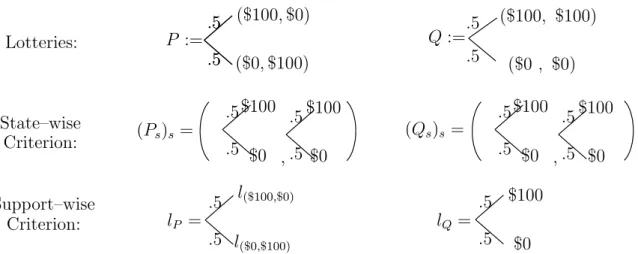
a state realizes. For example, P in Figure 1 is the fifty-fifty ex-ante mixture of ($100,$0) and ($0,$100). This type of mixture is henceforth indicated by ⊕. The other is an
ex-l :.5($100,$0) +.5($0,$100)≡ .5 .5 ($0 , $100) ($100, $0) .5 .5 $100 $0 .5 .5 $100 $0 , P :.5($100,$0)⊕.5($0,$100)≡
Figure 1: Ex-ante Mixture P and Ex-post Mixture l
post mixture, or a state-wise mixture of payoff profiles, which is a randomization after a state realizes. For example, l in Figure 1 is the fifty-fifty ex-post mixture of ($100,$0) and ($0,$100). This type of mixture is henceforth indicated by +, as is conventional literature. Under each context, the difference between the mixtures is crucial, as will be explained in detail later: under ambiguity aversion, an ex-ante mixture could provide only ex-ante hedging but not ex-post hedging. This could be the reason why, in some experiments, some people, who prefer ex-post mixtures, are averse to ex-ante mixtures. Also, under inequality aversion, an ex-ante mixture could provide only ex-ante equality but notex-post equality.
However, in Anscombe and Aumann (1963), the Reversal of Order axiom implies that an ex-ante mixture is indifferent with its ex-post mixture, i.e., αf⊕(1−α)g ∼αf+ (1−α)g
3For instance, in the context of ambiguity aversion, see Dominiak and Schnedler (2009), Spears (2009),
and Dwenger et al. (2010). For examples, in the context of inequality aversion associated with other-regarding preferences, see Bolton and Ockenfels (forthcoming), Krawczyk and Le Lec (2008), and Kircher, Luding, and Sandroni (2009). These experiments are discussed in detail in Section 2
for any payoff profiles f and g, and, α ∈ [0,1]. Hence, this axiom precludes the study of a preference for ex-ante mixtures separately from a preference for ex-post mixtures.
For the above reason, we do not assume the Reversal of Order axiom. Instead, we propose a new weaker axiom, the Indifference axiom. To see the difference between these axioms, notice that one way to justify the Reversal of Order axiom is by a state-wise evaluation: if you look at P state-wise, it offers the same lottery asl. As will be explained in Section 1.1, the criterion has been implicitly used by Raiffa (1961) in his famous critique of ambiguity aversion.
There is, however, another natural comparison between P and l: if you look at each payoff profile in the support ofP, it offers nonconstant payoff profiles, namely ($100,$0) and ($0,$100), which would be less attractive than the constant payoff profilel under ambiguity aversion as well as under inequality aversion;4 this way of evaluation is called
support-wise evaluation. The Indifference axiom states that if two lotteries on payoff profiles are indifferent according to both the state-wise and the support-wise criteria, then the lotteries should be indifferent.
Using the Indifference axiom together with standard axioms, two preferences are charac-terized for each context respectively: for ambiguity aversion, we axiomatize EAP Maxmin preference shown as (2) in Section 1.1, which is an extension of Gilboa and Schmeidler’s (1989) Maxmin preferences. For inequality aversion, on the other hand, we axiomatize
EAP Piecewise preferences shown as (3) in Section 1.2, which is an extension of Fehr and Schmidt’s (1999) Piecewise preferences.
Both representations have a similar structure. To see this, letP be any ex-ante mixture with finite support. Then, P = P(f1)f1 ⊕ · · · ⊕P(fn)fn, where P(fi) is the probability assigned to payoff profile fi by P. Then, for each state s, the marginal distribution of P
on s is Ps =P(f1)fs1+· · ·+P(fn)fsn, where fsi is the payoff at s in fi. Hence, the payoff
profile (Ps)s, which offers Ps at each state s, summarizes an ex-ante evaluation of P before
4In a social context, under which inequality aversion matters, states are reinterpreted as individuals. So,
a state realizes. Given the notations, the general representation can be presented as follows: V(P) =δ U((Ps)s ) + (1−δ) ∫ F U(f)dP(f), (1)
where δ is a real number and U is a real-valued function on the set F of payoff profiles. In the representation (1), the function U captures a preference for ex-post mixtures as in Maxmin preferences or in Piecewise preferences. Given U, on the other hand, the real number δ captures a preference for ex-ante mixtures in each context, as will be explained in Section 1.1 and 1.2, respectively.5 To see this, note that δ is the relative weight between the first and the second terms, where the first term is a utility associated with the ex-ante evaluation, while the second term is a utility associated with the ex-post evaluation
because, in the second term, each ex-post payoff profile in the support of P is evaluated by U separately.
Indeed, the representation (1) satisfies the Reversal of Order axiom if and only ifδ= 1. Given that our purpose is to develop a model which does not satisfy the Reversal of Order axiom, one might wonder why it does not suffice to consider the simpler special case in which δ= 0. However, this special case trivially implies the Independence axiom on ex-ante mixtures so that there is no strict preference for ex-ante mixtures.
The remainder of Section 1 is organized as follows: Section 1.1 provides an overview of EAP Maxmin preferences; while, Section 1.2 provides an overview of EAP Piecewise preferences; finally, in Section 1.3, the related literature is discussed. Next, Section 2 reviews recent experimental evidence on a preference for ex-ante mixtures under the two types of aversion. After that, Section 3 introduces the setup. Then, EAP Maxmin preferences are characterized in Section 4, while in Section 5, EAP Piecewise preferences are characterized. In Section 6, EAP Maxmin and EAP Piecewise preferences are applied to games. Finally in Section 7, further relationships among the axioms of Anscombe and Aumann (1963), Seo (2009), and our model are investigated. All proofs are in the appendix.
1.1
EAP Maxmin preferences
Ellsberg (1961) proposed the following thought experiment: consider two urns, one of which we call objective and the other of which we call ambiguous. Each urn contains 100 balls, each of which is either red or black. The objective urn contains 50 black and 50 red balls. There is no further information about the contents of the ambiguous urn. You first decide which urn you will draw from; then you bet on the color of the ball that you will draw, and you then draw a ball. If your bet turns out to be correct, you will get $100. Typically, subjects strictly prefer the objective urn than the ambiguous urn. This behavior is called
ambiguity aversion.
Raiffa (1961) criticizes ambiguity-averse preferences as follows: by flipping a coin to choose on which color in the ambiguous urn to bet, you can obtain an ex-ante mixture P that is shown in Figure 2. If you look at P state-wise, it offers the same lottery that the
.5 .5 P := ($0 , $100) ($100, $0) l := .5 .5 $100 $0 Figure 2: Flipping a Coin to Make a Decision
objective urn offers, namely, which shown asl in Figure 2. So,P andlshould be indifferent. Hence, there is no reason why you strictly prefer the objective urn.
As Raiffa’s (1961) argument suggests, some people might prefer flipping a coin and then deciding. One conceivable justification for such a preference is that ex-ante mixtures provide hedging in ex-ante expected payoffs. When a coin is flipped, the ex-ante expected payoff for each color becomes a constant $50, although the decision maker finally ends up with the ambiguous bets ex post. We call this preference for ex-ante mixtures ex-ante ambiguity aversion. In contrast, conventional ambiguity aversion constitutes a preference for ex-post mixtures.6 Henceforth, we call this conventional ambiguity aversion ex-post
ambiguity aversion. Indeed, recent experiments, reported in Dominiak and Schnedler (2009) and Spears (2009), have found that subjects often have different attitudes toward ex-ante
and ex-post ambiguity.
Using the Indifference axiom together with standard axioms used in Gilboa and Schmei-dler (1989), we characterize Ex-ante/Ex-post (EAP) Maxmin preferences that capture ex-ante ambiguity aversion and also, but separately, ex-post ambiguity aversion as follows:
V(P) =δ min µ∈C ∫ S ( ∫ F u(fs)dP(f) ) dµ(s) + (1−δ) ∫ F ( min µ∈C ∫ S u(fs)dµ(s) ) dP(f), (2)
where S is the set of states, C is a subset of the set of all finitely additive probabilities on S, and u is a von Neumann-Morgenstern utility function.
In the representation (2), the set C of priors captures ex-post ambiguity aversion as in Gilboa and Schmeidler (1989). On the other hand, the relative weight δ between the first and the second termrs captures ex-ante ambiguity aversion, as will be formally shown in Section 4.4. To see this, observe that in the first term, minimum is taken outside of the integral not only with respect to ex-post mixtures but also with respect to ex-ante mixtures, in contrast to in the second term. So, in the first term, ex-ante mixtures provide hedging as much as ex-post mixtures, as opposed to in the second term.
1.2
EAP Piecewise Preferences
Another situation in which people typically prefer ex-ante mixtures is a social environment in which inequality matters. A classical example of “Machina’s (1989) mom” captures the essence of such a preference as follows: a mother has one indivisible good, which worths, say, $100. She has to give it either to her daughter or to her son. She is indifferent between the choices. In such a situation, she would prefer flipping a coin in order to make a decision; then she obtains an ex-ante mixture P on allocations over the children that is shown in Figure 2 again.
The rationale of such preferences would be that ex-ante mixtures provideex-ante equality, or equality in ex-ante expected payoffs. In the example of “Machina’s (1989) mom”, when a coin is flipped, the ex-ante expected payoff for each child becomes the same $50, although the mother finally ends up with the unequal allocations ex post. We call this preference
for ex-ante mixturesex-ante inequality aversion. In contrast, ex-post mixtures even provide
ex-post equality, or equality in ex-post payoffs; so, we call a preference for ex-post mixtures
ex-post inequality aversion.
Indeed, as will be discussed in Section 2.2, such preferences for ex-ante mixtures as well as for ex-post mixtures have been observed in many recent experiments on other-regarding preferences. One robust finding in the experimental studies is that such preferences are nonmonotonic with respect not only to ex–ante expected payoffs but also to ex–post payoffs. For example, in ultimatum games, almost half of recipients, on average, reject positive but unfair offers by dictators, which is less than 20 percent of a total prize; and thereby both of the recipients and dictators obtain nothing. (See Fehr and Schmidt (2005) for a survey.) Such behavior is inconsistent with Gilboa and Schmeidler’s (1989) Maxmin preferences, which are monotonic with respect to ex-post payoffs.7
To describe such experimental evidence parsimoniously, using the Indifference axiom again, together with standard axioms, we characterize Ex-ante/Ex-post (EAP) Piecewise preferences that capture ex-ante inequality aversion and also, but separately, ex-post in-equality aversion as follows:
V(P) =δ ( EPu(f1)− ∑ s̸=1 ( αsmax{EPu(fs)−EPu(f1),0}+βsmax{EPu(f1)−EPu(fs),0} )) + (1−δ) ∫ F ( u(f1)− ∑ s̸=1 ( αsmax{u(fs)−u(f1),0}+βsmax{u(f1)−u(fs),0} )) dP(f), (3)
where 1 ∈ S denotes the decision maker, αs, βs are nonnegative real numbers, u is a von
Neumann-Morgenstern utility function, and EPu(fs) =
∫
Fu(fs)dP(f). Under the
assump-tion of the risk neutrality, EAP Piecewise preferences reduce to the utility funcassump-tion proposed by Fehr and Schmidt (1999), for degenerate lotteries on allocations.
In the representation (3), the nonnegative numbersαsand βscapture ex-post inequality
aversion as in Fehr and Schmidt (1999). In particular, αs and βs are interpreted as indices
7As for a planner’ social preferences, however, it would be reasonable to assume monotonicity with
respect to ex-post payoffs. So, EAP Maxmin preferences would be consistent with such preferences. Indeed, it is easy to see that if δ ∈(0,1), EAP Maxmin preferences can describe the choice of “Machina’s (1989) mom”.
of disutility from envy and guilt toward the individual s when the decision maker gets less and more, respectively than the individual s. Given this, the relative weight δ between the first and the second terms captures ex-ante inequality aversion, as will be formally shown in Section 5.4. To see this, note that the first term represents a concern about ex-ante equality, because the term depends on the differences in the expected utilities, while the second term captures a concern about ex-post equality, because the term depends on the differences in the ex-post utilities.
1.3
Related Literature
To our knowledge, no other axiomatic papers have studied ex-ante mixtures and ex-post mixtures in the context of a preference for randomization.
However, there are a few axiomatic papers which relax the Reversal of Order axiom. Among them, to the best of our knowledge, the first is Dr`eze (1987), which studies the issue in a context of games with moral hazard. A recent paper that is most closely related to the present paper is Seo (2009).8 He does not assume the Reversal of Order axiom either. However, under Seo’s key axiom, Dominance, the Reduction of Compound Lotteries axiom
implies the Reversal of Order axiom. This means that, in Seo’s model, the distinction between ex-ante mixtures and ex-post mixtures is impossible as long as we assume the standard assumption on the reduction.
In contrast, under the Indifference axiom, this incompatibility does not arise, because, as will be shown in Section 7, the Indifference axiom is weaker than the Reversal of Or-der axiom, thereby enabling the distinction between the two types mixtures, but it is still stronger than the Reduction of Compound Lotteries axiom. Indeed, there is a direct con-nection between the Indifference axiom and the Dominance axiom: under the Reduction of Compound Lotteries axiom, the Dominance axiom implies the Indifference axiom but not vice versa, as will be shown in Section 7.
In terms of applications, the present paper is related to a literature on game theory
that studies ambiguity-averse players, in which mixed strategies correspond to lotteries on acts. The special cases of EAP Maxmin preferences and EAP Choquet preferences (Choquet counterpart of EAP Maxmin), where δ = 0 or 1, have been used in the literature as follows:9 Klibanoff (1996) and Lo (1996) have applied EAP Maxmin preferences with
δ = 1; Eichberger and Kelsey (2000) have applied EAP Choquet preferences with δ = 0; Mukerji and Shin (2002) have applied EAP Choquet preferences with δ= 0 as well as with δ = 1. As these authors note, both assumptionsδ= 1 andδ= 0 could provide unintuitively extreme predictions in some games, respectively. In such games, in Section 6, it will be shown that, δ ∈ (0,1) could predict more reasonable behavior of ambiguity-averse players than δ = 0 and 1.
Finally, the present paper is also related to the social choice literature regarding the trade-off between equality of opportunity and equality of outcome; these issues are addressed especially in Ben-Porath, Gilboa, and Schmeidler (1997) and Gajdos and Maurin (2004).10 However, the models and motivations in both papers are different from ours. These papers have considered a social planner’s preferences on matrices of real numbers that are utilities over a product space that consists of states and individuals. Hence, in their model, there is no conceptual counterpart of ex-ante mixtures.11 In addition, our emphasis in this paper is other-regarding preferences, not a planner’s social preferences, in response to recent rich experimental evidence on the former; the present is the first paper apart from Saito (2008) to provide an axiomatization of the utility function proposed by Fehr and Schmidt (1999).
2
Experiments
As noted, both EAP Maxmin and EAP Piecewise preferences are consistent with recent experimental evidence in each context.
9Since Choquet expected utilities with convex capacity have Maxmin representations, our axiomatization
of EAP Maxmin preferences is also an axiomatize EAP Choquet preferences with convex capacities.
10Ben-Porath et al. (1997) do not provide an axiomatization. Gajdos and Maurin (2004) axiomatize
a weaker representation than the one used in Ben-Porath et al. (1997). The representations and axioms proposed by Gajdos and Maurin (2004) are different from ours.
2.1
EAP Maxmin Preferences in Experiments
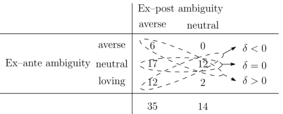
EAP Maxmin preferences can parsimoniously describe experimental evidence found by Do-miniak and Schnedler (2009). They have studied relationship between attitudes toward ex-ante and ex-post ambiguity. The number in Table 1 shows the number of subjects who exhibited a corresponding attitude toward ex-ante and ex-post ambiguity.12
averse loving neutral averse neutral Ex–post ambiguity Ex–ante ambiguity 6 17 12 35 0 12 2 14 δ <0 δ = 0 δ >0
Table 1: Attitudes toward Ex-ante and Ex-post Ambiguity
Dominiak and Schnedler’s (2009) experimental result might be summarized by the follow-ing two points. First, subjects who are averse to ex-post ambiguity differ in their attitudes toward ex-ante ambiguity. This result is inconsistent not only with the Reversal of Order axiom but also with Raiffa’s (1961) critique because his claim implies that all of the ex-post ambiguity-averse decision makers should be ex-ante ambiguity averse as well. Second, however, most of the ex-post ambiguity neutral subjects are ex-ante ambiguity neutral as well.
The first observation is explained by the heterogeneity of the parameter δ as follows: suppose EAP Maxmin preferences exhibit ex-post ambiguity aversion. Then, as will be shown in Section 4.5, the preferences exhibit ex-ante ambiguity aversion, neutrality, and loving, if and only ifδ > 0,δ= 0, and δ <0, respectively, which is consistent with Table 1. The second observation is also consistent with EAP Maxmin preferences. As will be shown in Section 4.5, among EAP Maxmin preferences, ex-post ambiguity neutrality implies ex-ante ambiguity neutrality for any δ, which is also consistent with Table 1.
Spears (2009) independently conducted similar experiments to Dominiak and Schnedler (2009) and has obtained similar tendencies. On the other hand, in a field experiment, Dwenger et al. (2010) have found a significant evidence for ex-ante ambiguity aversion, which would suggest that δ >0.
2.2
EAP Piecewise Preferences in Experiments
EAP Piecewise preferences are also consistent with recent experimental evidence. Firstly, we discuss the experimental results in probabilistic dictator games, in which dictators al-locate chances to win a prize, in contrast to standard dictator games, in which dictators allocate a prize itself. One of the robust findings in such experiments is that a substantial fraction of dictators shared chances to win, so that exhibited ex-ante inequality aversion. This finding is simply described by EAP Piecewise preferences with δ > 0.13 See, for the
experiments, Karni, Salmon, and Sopher (2008), Bohnet, Greig, Herrmann, and Zeckhauser (2008), Bolton and Ockenfels (forthcoming), Krawczyk and Le Lec (2008), and Kircher et al. (2009).
Secondly, Kariv and Zame’s (2009) experiment is also consistent with EAP Piecewise preferences. In their experiments, subjects are asked to divide a budget z intox andy such thatx+qy≤z, whereqis a given price. After the decision, the payoff of the decision maker and a recipient are determined as x or y with the probability .5, so that what the decision maker obtains is an ex-ante mixture .5(x, y)⊕.5(y, x). Hence, the subjects are required to make decisions under a veil of ignorance.
One of their main findings is that most of the subjects did not allocate all funds to the cheaper element. This fact is also consistent with EAP Piecewise preferences. To see this, assume the risk neutrality, for simplicity. Then, the utility by the ex-ante mixture is as follows: V ( .5(x, y)⊕.5(y, x) ) = 1 2 [ (x+y)−(1−δ)(α+β)|x−y| ] . (4)
So, when (1−δ)(α+β) exceeds a certain level, in order to maximize the utility, the decision maker tries to equalize x and y even if the prices are not the same.14
Finally, EAP Piecewise preferences are also consistent with seemingly contradictory ex-perimental results on efficiency versus inequality; recently, a number of papers have claimed that efficiency, or the sum of allocation across agents, has a stronger influence than in-equality. In particular, Charness and Rabin (2002) report that in a dictator game, almost 50 percent of their subjects chose an efficient but unequal allocation (in which the dictator obtained 375 points and the receiver obtained 750 points) to an equal but inefficient allo-cation (in which each player obtained 400 points).15 This behavior seems contradictory to any theory of ex-post inequality aversion including a theory provided by Fehr and Schmidt (1999).
The key fact that can explain this contradiction by using EAP Piecewise preferences is that in the experiments that are in favor of efficiency, each subject makes decisions as if he were a dictator, but the actual roles (i.e., dictator or receiver) are determined at random. Hence, the subjects are required to make decisions under risk over roles.
Under the risk over roles, each subject has to face a game with the other subjects because their decisions could determine the subject’s payoff if a dictator is chosen among them. In a game that describes the aforementioned dictator game under the risk over roles, it will be shown in Section 6.2 that in an equilibrium, subjects with EAP Piecewise preferences choose the efficient allocation rather than the equal allocation because of the ex-ante equality.16
To understand this result intuitively, note thatrisk over roles plays a role similar to that of veil of ignorance. To see this, suppose that two subjects decide to allocatexto themselves and yto the other. Then, under the risk over roles, what they obtain is the ex-ante mixture
14Without loss of generality, consider the case where q <1. If 1−δ > q−1
(α+β)(q+1), then EAP Piecewise
preferences with such parameters are consistent with the experimental evidence that many subjects did not spend all the budget to the cheaper element, i.e.,y.
15See, for other experiments, Engelmann and Strobel (2004, 2006)
16Indeed, this result is consistent with experimental evidence found by Bolton and Ockenfels (2006), which
report that in three-person dictator games, under risk over roles, subjects tended to choose efficient but unequal allocations over equal but inefficient allocations.
.5(x, y)⊕.5(y, x). Thus, the utility of each subject is determined as in (4), in other words: V ( .5(x, y)⊕.5(y, x) ) = 1 2 [ (“efficiency”)−(1−δ)(α+β)(“inequality”) ] .
Hence, even if a subject cares about ex-post equality (i.e., α and β are positive), if he weighs ex-ante equality heavily enough (i.e.,δ is larger than a certain level), then his utility from choosing the efficient allocation becomes larger than his utility from choosing the equal allocation, given that the other player chooses the same efficient allocation. Therefore, it looks as if the subjects with EAP Piecewise preferences care more about efficiency than about inequality.
3
Setup
For any topological spaceX, let ∆(X) be the set of distributions overXwith finite supports. An element in ∆(X) is called a lottery onX. Let δx ∈∆(X) denote a point mass on x.
LetS be a set of states and let Σ be an algebra of subsets of S. Let Z denote a set of outcomes. Both set S and set Z are assumed to be nonempty. A payoff profile f is called an act and defined to be a Σ-measurable function from S into ∆(Z) with finite range. For each act f, we writefs∈∆(Z), instead of f(s). Let F be the set of all acts.
A preference relation % is defined on ∆(F). As usual, ≻ and ∼ denote, respectively, the asymmetric and symmetric parts of %. Aconstant act is an act f such thatfs =fs′ for
all s, s′ ∈ S. Elements in ∆(F) are denoted by P, Q, and R. For all P ∈ ∆(F), supp P is the support of P. Elements in F are denoted by f, g , and h. Elements in ∆(Z) are denoted byl, q, r and are identified as constant acts. For f ∈F, an elementlf ∈∆(Z) is a
certainty equivalent for f if f ∼lf.
Finally, ex-ante mixtures and ex-post mixtures are formally defined as follows:
Definition: For all α ∈ [0,1] and P, Q ∈ ∆(F), αP ⊕(1−α)Q ∈ ∆(F) is a lottery
on acts such that (αP ⊕(1−α)Q)(f) = αP(f) + (1−α)Q(f) ∈ [0,1] for each f ∈ F. This operation is called an ex-ante mixture. For degenerate lotteries on acts, we write
αf ⊕(1−α)g ∈∆(F), instead of αδf ⊕(1−α)δg, for any α∈[0,1], andf, g ∈F.
Definition: For all α ∈ [0,1] and f, g ∈ F, αf + (1−α)g ∈ F is an act such that
(αf + (1−α)g)(s)(z) =αf(s)(z) + (1−α)g(s)(z)∈ [0,1] for each s ∈S and z ∈Z. This operation is called an ex-post mixture.
4
EAP Maxmin Preferences
To characterize EAP Maxmin preferences, instead of Reversal of Order, we assume Indif-ference as well as the axioms used in Gilboa and Schmeidler (1989).
4.1
Axioms
The first six axioms are due to Gilboa and Schmeidler (1989). However, since Reversal of Order is not assumed, both Continuity and Certainty Independence are assumed for ex-ante mixtures and also, but separately, for ex-post mixtures.
Axiom 1 (Weak Order): % is complete and transitive. Axiom 2 (Continuity):
(i) For all P, Q, R ∈ ∆(F), if P ≻ Q and Q ≻ R, then there exist α and β in (0,1) such that αP ⊕(1−α)R≻Q and Q≻βP ⊕(1−β)R.
(ii) For all f, g, h ∈ F, if f ≻ g and g ≻ h, then there exist α and β in (0,1) such that αf + (1−α)h≻g and g ≻βf + (1−β)h.
Axiom 3 (Nondegeneracy): There exist z+, z− ∈Z such thatz+≻z−. Axiom 4 (Monotonicity): For all f, g∈F,
fs % gs for all s ∈S⇒f % g.
If a preference relation % satisfies the axioms above, then each act f ∈ F admits a certainty equivalent lf ∈∆(Z).
Axiom 5 (Ex-post Ambiguity Aversion): For all α∈[0,1] and f, g∈F,
f ∼g ⇒αf + (1−α)g % f.
Mixing constant acts, ex-ante as well as ex-post, does not provide any hedging. Hence,
Axiom 6 (Ex-ante/Ex-post Certainty Independence):
(i) For all α ∈(0,1], P, Q∈∆(F), and l∈∆(Z),
P % Q⇔αP ⊕(1−α)l % αQ⊕(1−α)l.
(ii) For all α ∈(0,1],f, g ∈F, and l ∈∆(Z),
f %g ⇔αf + (1−α)l % αg+ (1−α)l.
The final axiom is a weaker formalization of Raiffa’s (1961) critique. As noted in In-troduction, his argument corresponds to the state-wise criterion. First, to formalize the state-wise criterion, a preliminary concept is defined here:
Definition: For allP ∈∆(F) and s∈S,
Ps=P(f1)fs1+· · ·+P(f n
)fsn,
where P =P(f1)f1⊕ · · · ⊕P(fn)fn.
In words,Psis a reduced marginal distribution ofP ons. Kreps (1988, p. 106) as well as
Raiffa (1961) have proposed an act (Ps)s∈S, which offers Ps at each state s, as a reasonable
embedding ofP ∈∆(F) toF. Henceforth, we write (Ps)s, instead of (Ps)s∈S for simplicity.
The next embedding corresponds to the support-wise criterion as follows: remember that lf ∈∆(Z) is a certainty equivalent for an act f.
Definition: For allP ∈∆(F),
where P =P(f1)f1⊕ · · · ⊕P(fn)fn.17
Axiom 7 (Indifference): For allP, Q∈∆(F),
(i) (Ps)s ∼(Qs)s; and (ii) lP ∼lQ ⇒P ∼Q.
Indifference states that if two lotteries on acts are indifferent according to the two criteria
jointly, then the lotteries should be indifferent. As will be shown in Section 7, a stronger axiom without the condition (ii), which will be called State-wise Indifference, is equivalent to Reversal of Order. Since the stronger axiom, State-wise Indifference, corresponds to Raiffa’s (1961) critique, Indifference would be interpreted as a weaker formalization of his critique. ($100,$0) ($0,$100) P := $100 $0 .5 .5 (Ps)s = $100 $0 , l($100,$0) lP = l($0,$100) .5 .5 .5 .5 .5 .5 .5 .5 Q:=.5 .5 ($0 , $0) ($100, $100) $100 $0 .5 .5 (Qs)s = $100 $0 , .5 .5 $100 lQ = $0 .5 .5 Lotteries: State–wise Support–wise Criterion: Criterion:
Figure 3: State-wise Criterion and Support-wise Criterion
To see formally the difference between Indifference and Raiffa’s (1961) critique, consider two lotteries P and Q on acts in Figure 3; since (Ps)s = (Qs)s, P and Q are indifferent
according to State-wise Indifference. So, Raiffa would conclude that P and Q should be indifferent. According to the support-wise criterion, on the other hand, Qis better than P, because, under ambiguity aversion, lQ = ($100, .5; $0, .5) ≻ ($100,$0) ∼ ($0,$100) ∼ lP.
Hence, Indifference does notconclude that P and Q are indifferent.18
17Note that, in general, it is not true thatP∼l
P. However, for a degenerate lottery on acts,f ∼lδf ≡lf. So, there is no contradiction in the notations.
4.2
Representation
Before stating the result, we mention that the topology to be used on the space of finitely additive set functions on Σ is the weak* topology.
Theorem1: For a preference relation% on∆(F), the following statements are equivalent:
(i) The preference relation satisfies Axioms 1–7.
(ii) There exist a real number δ, a nonempty convex closed set C of finitely additive proba-bility measures on Σ, and a nonconstant mixture linear function u : ∆(Z)→ R, such that
% is represented by the function V : ∆(F)→R of the form
V(P) =δ min µ∈C ∫ S ( ∫ F u(fs)dP(f) ) dµ(s) + (1−δ) ∫ F ( min µ∈C ∫ S u(fs)dµ(s) ) dP(f).
Definition: A preference relation%on ∆(F) is called anEx-ante/Ex-post (EAP) Maxmin
preference if it satisfies axioms in (i) of Theorem 1.
By Theorem 1, EAP Maxmin preferences can be represented by a triple (δ, C, u). Next, we give the uniqueness property of this representation.
Corollary 1: The following two statements are equivalent:
(i) Two triples (δ, C, u) and (δ′, C′, u′) represent the same EAP Maxmin preference as in Theorem 1.
(ii) (a) C =C′, and there exist real numbersα and β such that α >0and u=αu′+β; and (b) If C is nondegenerate, then δ=δ′.
4.3
Characterizations of
δ
The parameter δ has a direct behavioral characterization in terms of ex-ante ambiguity aversion and interim ambiguity aversion:
Axiom (Ex-ante Ambiguity Aversion): For allα ∈(0,1) and f, g∈F,
f ∼g ⇒αf ⊕(1−α)g %f.
Ex-ante ambiguity neutrality andex-ante ambiguity loving are defined in the same way by changing the right-hand side of the definition toαf⊕(1−α)g ∼f and tof %αf⊕(1−α)g, respectively.
Axiom (Interim Ambiguity Aversion): For allα∈(0,1) and f, g∈F,
αf + (1−α)g % αf ⊕(1−α)g.
Interim ambiguity aversion means that an ex-post mixture is preferred over its ex-ante mixture. This is because an ex-post mixture provides hedging in ex-post utilities, whereas an ex-ante mixture provides hedging only in ex-ante expected utilities. In addition,interim ambiguity neutrality is defined in the same way by changing % to ∼, which is nothing but Reversal of Order among two acts.
Proposition 1: Suppose% is an EAP Maxmin preference with nondegenerate C.
(i) % exhibits ex-ante ambiguity aversion if and only if δ≥0. (ii) % exhibits interim ambiguity aversion if and only if δ ≤1.
Note that given the representation, it is easy to see that EAP Maxmin preferences with δ = 0 and δ = 1 satisfy ex-ante ambiguity neutrality and interim ambiguity neutrality, respectively.
4.4
Comparative Attitudes toward Ex-ante Ambiguity
We now study comparative attitudes toward ex-ante ambiguity.
Definition: Given two preference relations %1 and %2, %1 is said to be more ex-ante
ambiguity averse than %2 if, for every P ∈∆(F) and every f ∈F,
P %2 f ⇒P %1 f.
The next proposition shows thatδ captures the attitude toward ex-ante ambiguity.
ui)}i=1,2, whereC1 andC2 are nondegenerate. Then, the following statements are equivalent:
(i) %1 is more ex-ante ambiguity averse than %2.
(ii)δ1 ≥δ2,C1 =C2, and there exist real numbersαandβsuch thatα >0andu1 =αu2+β.
Note that in (ii), both of the preferences coincide inCas well as inuunder normalization. Therefore, Proposition 2 says that stronger ex-ante ambiguity aversion is characterized only by a larger value of δ. Therefore, δ can be interpreted as an index of ex-ante ambiguity aversion.
4.5
Relation between Attitudes toward Ex-ante and Ex-post
Am-biguity
To conclude this section, implications of EAP Maxmin preferences on the relation between attitudes toward ex-ante and ex-post ambiguity are characterized. In particular, it will be shown that the implications of EAP Maxmin preferences are consistent with Dominiak and Schnedler’s (2009) experimental evidence, which was summarized by two points in Table 1 as follows. Fistly, among ex-post ambiguity averse subjects, the attitude toward ex-ante ambiguity is quite heterogeneous; but secondly most ex-post ambiguity-neutral subjects are ex-ante ambiguity neutral as well. These results are formally described by EAP Maxmin preferences as follows:
Proposition 3: Suppose % is an EAP Maxmin preference.
(i) (a) Suppose δ >0. Then, % exhibits ex-post ambiguity aversion if and only if % exhibits ex-ante ambiguity aversion.
(b) Suppose δ <0. Then, % exhibits ex-post ambiguity aversion if and only if % exhibits ex-ante ambiguity loving.
(c) Suppose δ= 0. Then, % exhibits ex-ante ambiguity neutrality.
(ii) For any δ, if % exhibits ex-post ambiguity neutrality, then % exhibits ex-ante ambiguity neutrality.
Part (i) shows that the heterogeneity observed in the experiment can be described sim-ply by whether or not δ is positive. Part (ii) shows that among EAP Maxmin preferences,
ex-post ambiguity neutrality implies ex-ante ambiguity neutrality, as observed in the exper-iment.
5
EAP Piecewise Preferences
In this section, EAP Piecewise preferences are characterized. Accordingly, the setSof states is assumed to be finite and reinterpreted as individuals including a decision maker, who is denoted by 1∈S.
5.1
Axioms
The axioms for EAP Maxmin preferences are now modified to capture inequality aversion. No modification is necessary for Indifference, and the first two modifications required are minor.
As noted in Section 1.2, to capture inequality aversion, Monotonicity (Axiom 4) needs to be weakened as follows:
Axiom 4’ (Substitution): For allf, g ∈F,
fs∼gs for all s ∈S⇒f ∼g.
The second minor change is that the following axiom is assumed instead of Ex-post Ambiguity Aversion (Axiom 5).
Axiom 5’ (Ex-post Inequality Aversion): Let l0 = 12δz+ +
1
2δz−. For alls̸= 1,
(i) (l0,(l0)−s) %(z+,(l0)−s); and
(ii) (l0,(l0)−s) %(z−,(l0)−s).19
Part (i) captures the disutility that results fromenvytoward the individual s when only the individual s is better off than the decision maker, while part (ii) captures the disutility
19For any lottery l, r∈∆(Z) ands∈S, (l,(r)
−s) is an act which offersl for the individuals and offers
that results from guilt toward the individual s when only the individual s is worse off than the decision maker.
The final axiom that requires a modification is Ex-ante/Ex-post Certainty Independence (Axiom 6). Specifically, a new weaker version of comonotonicity needs to be defined. Re-member that 1∈S denotes the decision maker.
Definition: Two acts f, g ∈ F are said to be pointwise comonotonic if for no s ∈ S,
f(s)≻f(1) and g(s)≺g(1).
Suppose two acts f and g are pointwise comonotonic. Then, the rank of utilities of any individual with respect to the decision maker is not reversed between f and g.20 Hence,
Axiom 6’ (Ex-ante/Ex-post Pointwise Comonotonic Independence):
(i) For all α ∈ (0,1] and P, Q, R∈ ∆(F) such that (Ps)s,(Rs)s, and (Qs)s,(Rs)s are each
pointwise comonotonic,
P % Q⇔αP ⊕(1−α)R % αQ⊕(1−α)R.
(ii) For allα∈(0,1] andf, g, h∈F such thatf, h, andg, hare each pointwise comonotonic,
f % g ⇔α f + (1−α)h % αg+ (1−α)h.
As noted, no modification is necessary for Indifference. The interpretation of that axiom is straightforward here. The first criterion (i) corresponds to ex-ante equality, because each marginal distribution Ps yields ex-ante expected payoff of the individual s. The second
criterion (ii) corresponds to ex-post equality, because each certainty equivalent lf reflects
the ex-post equality of f. Hence, Indifference means that if two lotteries P and Q on acts are indifferent in both ex-ante and ex-post equality, then P and Q should be indifferent.
20Schmeidler (1989, p. 586) has presented an interpretation ofcomonotonicity from the point of view of a
planner’s social preferences as follows: two income allocationsf andgare comonotonic if the social rank of any two agents is not reversed betweenf andg. When we focus on anagent’s other-regarding preferences, what is relevant to the agent is social rankwith respect to the agent himself, not the social rank ofany two agents.
5.2
Representation
Theorem2: For a preference relation% on∆(F), the following statements are equivalent:
(i) The preference relation satisfies Axioms 1, 2, 3, 4’, 5’, 6’, and 7.
(ii) There exist a real number δ, nonnegative numbers {αs, βs}s̸=1, and a nonconstant
mix-ture linear functionu: ∆(Z)→Rsuch that%is represented by the functionV : ∆(F)→R
of the form V(P) =δ ( EPu(f1)− ∑ s̸=1 ( αsmax{EPu(fs)−EPu(f1),0}+βsmax{EPu(f1)−EPu(fs),0} )) + (1−δ) ∫ F ( u(f1)− ∑ s̸=1 ( αsmax{u(fs)−u(f1),0}+βsmax{u(f1)−u(fs),0} )) dP(f), whereEPu(fs) = ∫
Fu(fs)dP(f). Furthermore, the two quadruples(δ, α, β, u)and(δ′, α′, β′, u′)
represent the same preference as in the above if and only if (α, β) = (α′, β′), δ = δ′ if
(α, β)̸=0, and there exist real numbers a and b such that a >0 and u=au′+b.
Definition: A preference relation % on ∆(F) is called an Ex-ante/Ex-post (EAP)
Piece-wise preference if it satisfies axioms in (i) of Theorem 2.
5.3
Characterization of
δ
The parameterδ has a direct behavioral characterization in terms of bothex-ante inequality aversion and interim inequality aversion, as follows:
Axiom(Ex-ante Inequality Aversion):For alls ̸= 1 andl+, l− ∈∆(Z) such thatl+ ≻l0 ≻l−,
(l+,(l0)−s)∼(l−,(l0)−s)⇒
1
2(l+,(l0)−s)⊕ 1
2(l−,(l0)−s) %(l+,(l0)−s).
Ex-ante inequality aversion means that an ex-ante mixture of unequal allocations offsets the inequalities in the expected utilities. So, the ex-ante mixture would be more desirable.21
21Ex-ante inequality aversion is consistent with the experimental evidence, drawn from the probabilistic
dictator games, that subjects who are indifferent between winning and losing tend to prefer flipping a coin to decide the winner.
In addition, ex-ante inequality neutrality is defined by changing % to ∼ in the right-hand side of the above definition.
Axiom (Interim Inequality Aversion): For alls ̸= 1,
1 2(z+,(l0)−s) + 1 2(z−,(l0)−s)% 1 2(z+,(l0)−s)⊕ 1 2(z−,(l0)−s).
To interpret interim inequality aversion, recall thatl0 = 12δz++
1
2δz−, so that the ex-post
mixture in the left hand side is identical to constant actl0 and provides ex-post equality. On
the other hand, the ex-ante mixture in the right hand side could provide ex-ante equality but not ex-post equality. So, the ex-post mixture would be preferred over the ex-ante mixture. In addition, interim inequality neutrality is defined by changing % to∼.
Corollary 2: Suppose% is an EAP Piecewise preference with (α, β)̸=0.
(i) % exhibits ex-ante inequality aversion if and only if δ≥0. (ii) % exhibits interim inequality aversion if and only if δ ≤1.
Note that given the representation, it is easy to see that EAP Piecewise preferences with δ= 0 and δ= 1 satisfy ex-ante inequality neutrality and interim inequality neutrality, respectively.
5.4
Comparative Attitudes toward Ex-ante Inequality
To conclude this section, comparative attitudes toward ex-ante inequality are characterized. As mentioned in Introduction, a preference for ex-ante mixtures is due to ex-ante inequality aversion in a social context, in contrast to ambiguous situations, in which such a preference is due to ex-ante ambiguity aversion. So, the same definition of being more ex-ante ambiguity averse in Section 4.4 is interpreted as the definition of beingmore ex-ante inequality averse
in the context of inequality aversion.
Hence, results analogous to those derived from Proposition 2 in Section 4.4 also hold for inequality aversion.
ui)}i=1,2, where (α1, β1)̸=0̸= (α2, β2). Then the following statements are equivalent:
(i) %1 is more ex-ante inequality averse than %2.
(ii) δ1 ≥ δ2, (α1, β1) = (α2, β2), and there exist real numbers a and b such that a > 0 and
u1 =au2+b.
Note that in (ii), both of the preferences coincide in α and β as well as in u under a normalization. Therefore, Corollary 3 says that stronger ex-ante inequality aversion is characterized only by larger value of δ. Therefore, δ can be interpreted as an index of ex-ante inequality aversion in a social context.
6
Games
In preceding sections, we saw how EAP Maxmin and EAP Piecewise preferences are con-sistent with many experimental results, mainly on single-person decision making. In this section, EAP Maxmin and EAP Piecewise preferences are applied to games in order to see the implications of the models in strategic situations.
6.1
EAP Maxmin Preferences in Games
As noted in Introduction, the special cases of EAP Maxmin and EAP Choquet preferences, whereδ= 0 or 1 have been used in the game theory literature on ambiguity-averse players.22
The following two symmetric games, Game I and Game II, suggest that δ ∈ (0,1) would predict more realistic behavior of ambiguity-averse players than δ = 0 and 1, respectively. The numbers in the games are von Neumann-Morgenstern utilities andxandεare a positive numbers.
22To see the relationship between the literature and our model, fix a game and a player. Then, the
player’s pure strategy corresponds to an act; the set of strategies of the other players corresponds to the set of states; hence, the player’s mixed strategies corresponds to ex-ante mixtures on acts.
1\2 d e a 2x 0 b 0 2x 1\2 d e a 2x 0 b 0 2x c x−ε x−ε Game I Game II
For both of the games, when they are played for the first time, the symmetry makes it difficult for each player to have a unique prior probability over the opponent’s strategies. So, in Game I, the ambiguity-averse players would prefer mixed strategies over pure strategies in order to hedge. In addition, in Game II, if a positive numberεis less than a certain threshold, player 1 would prefer strategyc, whose payoff is constant, over any mixed strategies between a and b.
EAP Maxmin preferences with δ ∈ (0,1) can describe these reasonable behaviors in a
strict equilibrium in each game as opposed to withδ = 0 and 1.23 EAP Maxmin preferences
withδ= 0 show that in Game I, if a player is indifferent between the strategies, then there is no strict incentive to mix between them. In addition, EAP Maxmin preferences with δ= 1 show that in Game II, for player 1, the fifty-fifty mix between a and b strictly dominates c for any small positive number ε.
6.2
EAP Piecewise Preferences in Games
In this section, we show that EAP Piecewise preferences can describe seemingly contra-dictory experimental results on efficiency versus inequality. As mentioned in Introduction, the key to resolving the putative contradiction is that it is only in the experiments that are strongly in favor of efficiency that subjects are under risk over roles. That is, in the experiments, each subject makes a decision as if he were a dictator, but actual roles (i.e., dictator or receiver) are determined at random.
23See Klibanoff (1996) for a definition of an equilibrium with ambiguity-averse players. He assumesδ= 1
We study a Bayesian game that describes the dictator game from Charness and Rabin (2002), mentioned in Section 2.2. In the game, they report that about 50 percent of the subjects chose the efficient but unequal allocation rather than the equal but inefficient al-location. Assume, for simplicity, there exist two players {1,2} and two types of players as follows: fair (i.e., αF, βF > 0 and δF > 0) and selfish (i.e., αS = 0 = βS). Player 1’s set of actions is {(375,750),(400,400)} and player 2’s set of actions is {(750,375),(400,400)}, where the first and second coordinates show the material prizes for players 1 and 2, re-spectively. Denote the efficient but unequal allocation by Ef, and the equal but inefficient allocation by Eq. The game is described as Game I in Figure 4.
.5(375,750)⊕.5(750,375) .5(375,750)⊕.5(400,400) .5(400,400)⊕.5(750,375) .5(400,400)⊕.5(400,400) Ef Eq Ef Eq Eq Ef 1 2 Game I (400,400) (375,750) Ef Eq 1 Game II Figure 4: Dictator Games with and without Risk over roles
In Game I, the player’s choice determines an allocation only if he turns out to be a dictator, in contrast to Game II, in which player 1’s choice determines an allocation for sure. So, given that each role is determined with the probability .5, what a player obtains is a fifty-fifty ex-ante mixture on allocations. For example, if player 1 chooses action Ef and player 2 chooses Eq, players obtain an ex-ante mixture that gives (375,750) and (400,400) with the probability .5. Now the result can be stated as follows:
Proposition 4: Suppose
(a) Players’ preferences are EAP Piecewise with u(z) = logz for all z ∈R+.
(b) There exist two types, fair (i.e., αF, βF >0,and δF >0)and selfish (i.e., αS = 0 =βS). Let αF =.2, βF =.9, and δF =.85. Then the following results hold:
(i) In Game I, there exists a Bayesian Nash equilibrium in which the fair type choose the efficient allocation (Ef ), the selfish type choose the equal allocation (Eq), and the common prior probability on the fair type is .5.
(ii) In Game II, for both types, choosing the equal allocation (Eq) strictly dominates choosing the efficient allocation (Ef ).
Note that in the result (i), the common prior probability on the fair type is consistent with the experimental evidence found by Charness and Rabin (2002), which report that about 50 percent of the subjects chose Ef.
Finally, to conclude this section, an implication of Proposition 4 on the use of risk over roles is discussed. Currently, in many experimental studies, subjects are required to make decisions under risk over roles. However, Proposition 4 shows that risk over roles induces subjects with EAP Piecewise preferences to choose the efficient allocations, even if they do not have a preference for efficiency itself. Indeed, this implication is consistent with the experimental evidence, found by Bolton and Ockenfels (2006), that under risk over roles, subjects tend to choose efficient but unequal allocations over equal but inefficient allocations.
7
Concluding Remarks on Axioms
To conclude the paper, the relationships among the key axioms used in Anscombe and Aumann (1963), Seo (2009), and our model are discussed. As noted, we will show that State-wise Indifference, which is a strengthening of Indifference by dropping the support-wise criterion, is equivalent with Reversal of Order. This result means that what makes the difference between Indifference and Reversal of Order is the support-wise criterion.
Based on the result above, we also show that Reversal of Order implies Indifference but not vice versa, and Indifference, in turn, implies Reduction of Compound Lotteries but not vice versa. This result clarifies the difference between Indifference and Seo’s Dominance. This is because, as noted, under Dominance, Reversal of Order and Indifference become equivalent; so, it is impossible to distinguish between ex-ante and ex-post mixtures as long as we assume the standard axiom on the reduction.
First, Reversal of Order by Anscombe and Aumann (1963) is formally defined as follows:
numbers such that ∑ni=1αi = 1,
α1f1⊕ · · · ⊕αnfn ∼α1f1+· · ·+αnfn.
As noted, Reversal of Order turns out to be equivalent to the following axiom:
Axiom (State-wise Indifference): For all P, Q∈∆(F),
(Ps)s∼(Qs)s⇒P ∼Q.
Lemma 1: Reversal of Order and State-wise Indifference are equivalent.
Note that State-wise Indifference is a strengthening of Indifference by dropping the requirement of the support-wise criterion. Hence,
Corollary 4:Reversal of Order implies Indifference.
As the example illustrated by Figure 3 in Section 4 shows, the opposite of Corollary 4 is not true. However, Indifference implies Reversal of Order among constant acts. Formally,
Axiom (Reduction of Compound Lotteries): For all set {li}ni=1 of lotteries and set {αi}ni=1
of nonnegative numbers such that ∑ni=1αi = 1,
α1l1⊕ · · · ⊕αnln ∼α1l1+· · ·+αnln.
Lemma 2: Indifference implies Reduction of Compound Lotteries.
As noted, Seo (2009) proposes an axiom of his own, Dominance, instead of Reversal of Order. To present the axiom, we must first introduce preliminary notations. For each f ∈ F and µ ∈ ∆(S), Ψ(f, µ) = µ(s1)fs1 +· · ·+µ(s|S|)fs|S| ∈ ∆(Z).
24 In addition, for
each P ∈ ∆(F) and µ ∈ ∆(S), Ψ(P, µ) = P(f1)Ψ(f1, µ)⊕ · · · ⊕P(fn)Ψ(fn, µ), where
P =P(f1)f1⊕ · · · ⊕P(fn)fn. Now, his axiom can be stated as follows:
Axiom (Dominance, Seo (2009)): For allP, Q∈∆(F),
Ψ(P, µ) % Ψ(Q, µ) for all µ∈∆(S)⇒P %Q.
Under Dominance, Seo (2009, p. 1587, Lemma 5.1) shows the equivalence between Reduction of Compound Lotteries and Reversal of Order for n = 2. This equivalence can be extended immediately to any finite n. This observation together with Corollary 4 imply the following result:
Corollary 5: Under Reduction of Compound Lotteries, Dominance implies Indifference.
Therefore, under Reduction of Compound Lotteries, Dominance together with the ax-ioms used in Theorems 1 and 2 (except Indifference) respectively imply EAP Maxmin and EAP Piecewise preferences with δ= 1.
Appendix: Proofs
Section A provides a sketch of the proofs of the sufficiencies for Theorems 1 and 2. Section B provides the proofs for Lemmas. The proofs of Theorem 1 and related results are in Section C, while Section D presents the proofs of Theorem 2 and related results.
A
Sketch of Proofs
First, a sketch of the proof for the sufficiency in Theorem 1 is provided. By the standard ar-gument, there exists a function V representing % on ∆(F), which is unique up to positive affine transformation. Ex-post Ambiguity Aversion, Ex-ante/Ex-post Certainty Indepen-dence, and Indifference will show that V can be taken so that the restriction U of V onF has a Maxmin representation. That is, there exists a set C of priors and a mixture linear function u on ∆(Z) such that U(f) = minµ∈C
∫
Then, for all P ∈∆(F), U((Ps)s) = min µ∈C ∫ S ( ∫ F u(fs)dP(f) ) dµ(s); U(lP) = ∫ F ( min µ∈C ∫ S u(fs)dµ(s) ) dP(f). (5)
Hence, it follows from Jensen’s inequality that U((Ps)s)≥U(lP) for all P ∈∆(F). Define
C = { (u(l), u(l))∈R2 ¯¯ l ∈∆(Z) } ; D ={(U((Ps)s), U(lP) ) ∈R2 ¯¯ P ∈∆(F)}. (6)
We now can show that C consists of the upper boundary of D as in Figure 5. In addition, if (x, y)∈D, (c, c)∈C, and α∈[0,1], then α(x, y) + (1−α)(c, c)∈D.
Define a binary relation ˆ% onD : for all (x, y),(x′, y′)∈D,
(x, y) ˆ% (x′, y′)⇔V(P)≥V(Q), where P, Q ∈ ∆(F), (U((Ps)s), U(lP) ) = (x, y), and (U((Qs)s), U(lQ) ) = (x′, y′). Indif-ference will show that %ˆ is a well-defined binary relation. The purpose of the proof is to show that there exists a real number δ such that for any (x, y) and (x′, y′) ∈ D, (x, y) ˆ% (x′, y′)⇔ δx+ (1−δ)y ≥δx′+ (1−δ)y′. Together with the definition of ˆ%, this implies that
V(P)≥V(Q)⇔δU((Ps)s) + (1−δ)U(lP)≥δU((Qs)s) + (1−δ)U(lQ).
Since bothV andU coincide withuon ∆(Z), it follows from the cardinal uniqueness of V that V(P) =δU((Ps)s) + (1−δ)U(lP) for all P, as desired.
In the following, we sketch how to show the existence of the desired real numberδ.25 It
will be shown that ˆ% satisfies completeness, transitivity, monotonicity onC, and certainty
25Note that, the continuity of ˆ%does not follow directly from the continuity of%. In addition, inR2, it
is well-known that in general, additive linear representation requires more than Independence. (See Debrue (1960).) So, the standard argument might not show the existence of the desiredδ directly.