Structured Rule Discovery from Heterogeneous Longitudinal Data for Complex Disease

(1)

STRUCTURED RULE DISCOVERY FROM HETEROGENEOUS

LONGITUDINAL DATA FOR COMPLEX DISEASE

A Thesis by ZHOU WANG

Submitted to the Office of Graduate and Professional Studies of Texas A&M University

in partial fulfillment of the requirement for the degree of MASTER OF SCIENCE

Chair of Committee, Peng Li

Co-Chair of Committee, Xiaoning Qian

Committee Members, I-Hong Hou

Xia Hu

Head of Department, Miroslav Begovic

December 2016

Major Subject: Computer Engineering

(2)

ABSTRACT

Many complex diseases manifest heterogeneous degenerative disease progression processes that impose enormous challenges for accurate disease prognosis and effective intervention. The emerging “big” data collected from the population with predisposed dis-ease risk brings us motivation to translate it into accurate prognosis and effective risk mon-itoring. We propose a structured sparse rule discovery method to identify risk-predictive patterns from heterogenous longitudinal. By extending the existing RuleFit framework, we have developed an analysis pipeline to derive risk-predictive patterns from complex data. The results in a de-identified Type 1 Diabetes dataset have shown promising predictive performances.

(3)

(4)

ACKNOWLEDGMENTS

Dr. Xiaoning Qian has been a great supervisor. His sage advice, insightful criticisms, and patient encouragement aided me with the whole process of this thesis in every way. I would like to thank Dr. Peng Li, Dr. I-Hong Hou, and Dr. Xia Hu whose support of this project was greatly needed and deeply appreciated. I am also grateful for the help and advice from Dr. Shuai Huang at the University of Washington. The help from Drs. Kendra Vehik and Kristian Lynch is truly appreciated for the data from The Environmental Determinants of Diabetes in the Young (TEDDY) study.

(5)

NOMENCLATURE

AD Alzheimer’s Disease

PD Parkinson Disease

T1D Type 1 Diabetes

RF Random Forest

LASSO Least Absolute Shrinkage and Selection Operator

OGL Overlapped Group LASSO

OGAPS Office and Graduate and Professional Studies at Texas

A&M University

(6)

LIST OF FIGURES

FIGURE Page

1.1 Study Purpose . . . 3

2.1 General Decision Tree . . . 7

3.1 Proposed Pipeline . . . 16 4.1 K-M: Rule01 OGL . . . 26 4.2 K-M: Rule02 OGL . . . 27 4.3 K-M: Rule03 OGL . . . 27 4.4 K-M: Rule04 OGL . . . 28 4.5 K-M: Rule05 OGL . . . 28 4.6 K-M: Rule06 OGL . . . 29 4.7 K-M: Rule07 OGL . . . 29 4.8 K-M: Rule08 OGL . . . 30 4.9 K-M: Rule09 OGL . . . 30 4.10 K-M: Rule10 OGL . . . 31 4.11 K-M: Rule11 OGL . . . 31 4.12 K-M: Rule12 OGL . . . 32 4.13 K-M: Rule13 OGL . . . 32 4.14 K-M: Rule14 OGL . . . 33

(9)

4.15 K-M: Rule15 OGL . . . 33 4.16 K-M: Rule01 Lasso . . . 36 4.17 K-M: Rule02 Lasso . . . 36 4.18 K-M: Rule03 Lasso . . . 37 4.19 K-M: Rule04 Lasso . . . 37 4.20 K-M: Rule05 Lasso . . . 38 4.21 K-M: Rule06 Lasso . . . 38 4.22 K-M: Rule07 Lasso . . . 39 4.23 K-M: Rule08 Lasso . . . 39 4.24 K-M: Rule09 Lasso . . . 40 4.25 K-M: Rule10 Lasso . . . 40 4.26 K-M: Rule11 Lasso . . . 41 4.27 K-M: Rule12 Lasso . . . 41 4.28 K-M: Rule13 Lasso . . . 42 4.29 K-M: Rule14 Lasso . . . 42 4.30 K-M: Rule15 Lasso . . . 43

(10)

LIST OF TABLES

TABLE Page

4.1 The Top 15 Identified Rules from OGL · · · · 25

4.2 Log-Rank Test p-values of Top 15 Rules from OGL · · · · 34

4.3 The Top 15 Identified Rules from LASSO · · · · 35

(11)

1 INTRODUCTION

1.1 Background

Many degenerative complex diseases, such as autoimmune disorders (e.g., Type 1 Diabetes, Celiac Disease, Rheumatoid Arthritis, Multiple Sclerosis), chronic disease (e.g., Asthma, Cardiac Diseases), and neurodegenerative diseases (e.g., Alzheimer’s Disease (AD), Parkinson Disease (PD), Amyotrophic Lateral Sclerosis), usually exhibit heteroge-nous phenotypes. The exact causes of those complex diseases are still in debate. However, the increasing evidences in the literature [1, 2], indicate that the evolution to disease clinical onsets can be affected by various exogenous factors, such as different early-life environ-ment exposures including dietary as well as infection exposures. It is possible to intervene to delay [3], or even avoid the disease clinical onset if we can better model, understand, and predict the disease progression processes by identifying potential risk-predictive patterns from high-dimensional measurements of candidate genetic, biomolecular, clinical, as well as environmental risk factors.

Discovering risk-predictive factors residing in massive biomedical data that have been accumulated in existing clinical trials, is potentially helpful but also imposes enor-mous data analytic challenges. Take Type 1 Diabetes (T1D) as an example, several stud-ies have been conducted to collect large scale data for risk factor identification for T1D data. Translating such big and complex data to accurate and reproducible understand-ing complex diseases requires appropriate data analytic methods. One frequently applied method is to analyze risk variables over observable outcomes with logistic regression [4]. However, common logistic regression models generally examine average risk effects over whole group without considering complex structured patterns, which might hide in the sub-groups. Therefore, a rule-based analysis approach has recently been proposed to identify

(12)

baseline profile patterns, and synthesize these pattern for risk prediction [5]. Such rule-based analyses can help model potential nonlinear interactive effects among candidate factors for better risk-predictive factor identification. However, besides baseline profile factors, temporal changes from the collected longitudinal data that can also potentially be risk-predictive have not been carefully studied.

1.2 Problem Statement

The problem to be studied in this thesis is to develop a structured rule-based method to derive risk-predictive patterns from data featured with temporal measurements. The problem fits within the ongoing data-driven discovery to model, understand, predict, and treat complex diseases with the help of mixed types of data collected with heterogeneous binary, categorical, quantitative measurements at the baseline as well as across disease progression time.

There are a number of essential challenges in this study. First of all, we must integrate mixed types of measurements into a unified statistical model to identify risk-predictive patterns in a more systematic way. Beyond that, with longitudinal data, it is critical to appropriately model the dependency structures among temporal measurements for the cor-responding factors that may change over time. Finally, with high-dimensional measure-ments, it is necessary to select non-redundant risk-predictive patterns to avoid potential overfitting problems in risk factor identification.

To overcome these challenges, we integrate rule-based analysis [6] and Overlapped Group LASSO (OGL) [7] in this study.

Rule-based analysis brings some special advantages, in comparison with earlier stud-ies using logistic regression. First, deriving rules can be considered as a normalization step, which can convert diverse data types into consistent binary indicators in a supervised fash-ion. This naturally handles the problem of having mixed types of data and helps integrate

(13)

binary, categorical, and numeric variables or features by mapping them to binary outputs based on whether their values fall into interesting ranges with respect to the outcome of interest. Second, the derivation rules are dependent on derived value ranges by setting thresholds considering the disease risk outcome. This makes it possible to model nonlin-earity that is relevant to disease risk. Finally, the derived rules often involve two or more features. It incorporates interactions among features for risk prediction.

Applying Overlapped Group LASSO with rule-based methods helps to facilitate the flexibility to model the group dependency among rules and candidate factors. When lon-gitudinal data is to analyze with potential temporal dependecy, such consideration of stuc-tured dependency may help derive more robust and accurate risk-predictive patterns while avoiding overfitting to ensure that the identified rules are non-redundant and significant.

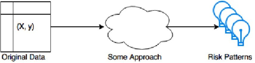
Figure 1.1: We want an approach to translate disease data into predictive patterns.

The purposes of this study are to 1) design a workflow(see Figure 1.1) to generate rules and appropriately select top rules as risk-predictive patterns for disease prognosis and risk monitoring to better understand and intervention of complex degenerative diseases; 2) evaluate the rule-based methods when deriving complex disease progression patterns from big, complex, and heterogenous data.

(14)

2 LITERATURE REVIEW

Biomarker and risk factor discovery has been studied extensively in the literature. Different statistical and computational methods have been proposed to analyze collected measurements to derive potential factors that may help understand and predict disease pro-gression and outcomes of interest.

2.1 Biomarker Discovery and Disease Prognosis

Logistic regression model has been the standard biostatistics method applied to study the association between disease outcome and candidate risk factors. As early as 1983, T.A. Welborn,et al. conducted a research [4] to identify risk factors for clinical macro-vascular diseases among diabetic subjects by applying a logistic regression method to determine the strength of association of possible risk variables over the outcome, clinical onset of macro-vascular diseases. In such association analyses, the logistic regression was performed for each variable, and the association was evaluated by the coefficient p-values, by which a subset of variables can be selected as “biomarkers” or “risk factors” considering the deviance contribution derived from the regression.

Logistic regression also has been implemented for disease prognosis. Another study in 2002 [8], by Bahman P. Tabaei,et al., proposed an empirical predictive equation for dia-betes screening by multiple logistic regression analysis. They collected data from subjects with no history of diabetes, assessed baseline characteristics, such as age, gender, height, weight, postprandial time, and estimated the likelihood of previously undiagnosed diabetes based on these candidate risk variables. The researchers finally developed a screening method for diabetes based on a predictive equation.

(15)

conducting logistic regression analysis have been mostly hypothesis-driven, by analyzing a limited number of carefully selected observable risk factors. For example, Welborn’s research validated that age is the major risk factor for macro-vascular disease among both Type 1 and Type 2 diabetic subjects, and plasma creatinine levels and plasma glucose levels are also significant risk predictors for Type 2 Diabetes subjects. However, many complex diseases are conjectured to be caused by both genetic and environmental risk factor expo-sures, as well as their interactions. Hypothesis-driven analyses may not reveal the disease progression mechanisms without accurate and systematic identification of all influencing factors. For example, in Welborn’s study, they failed to validate some well-recognized risk factors for vascular diseases, such as cigarette smoking. Although they claimed that this discrepancy may be caused by the crudity of simple smoking questionnaire, ignoring inter-active effects in traditional association analyses by logistic regression in their research may be one of the reasons that they failed to demonstrate the smoking effects on macro-vascular complications for diabetic subjects.

In order to integrating interaction in addition to individual effects for risk factor identification and disease prognosis, one way is to perform new logistic regressions on subgroups of the variables including their potential interaction terms. However, with the current trend of data-driven research to collect large-scale and high-dimensional observ-able measurements in biomedical studies, we face enormous data analytic challenges to do that. First, adding interaction terms can increase the model complexity and computational complexity in an exponential fashion. With often a limited number of samples in biomed-ical studies, it may lead to many false discoveries in addition to computational difficulty. When adding interaction terms with the help of experts or existing hypotheses, it may in-cur the cost from human labor and potential bias towards the analysis results. Second, with the availability of different types of measurements, it requires appropriate analytic methods to integrate all different types of data in one unified analysis framework to obtain

(16)

reproducible, interpretable, and meaningful results. Finally, when we have longitudinal measurements from prospective clinical trials, how to model the temporal dependency im-poses another potential challenge.

To overcome these analytic challenges, we adopt rule-based methods for risk factor identification when analyzing complex and heterogeneous data from biomedical studies. Rule-based methods [9] are based on decision trees. In the following, we give the liter-ature review on decision tree, random forest, and rule-based analytic methods and their applications in biomedical research.

2.2 Decision Tree

The decision tree classifiers are widely and successfully applied in diverse areas, e.g., biomedical engineering, financial analysis, system controls, software engineering. As stressed in S.R. Safavian’s survey paper [10], the most crucial property of a decision tree model is its capability to simplify complex decision-making process by a representation of sequences of comprehensible decision rules. A decision tree is a tree-like directed graph model, where each tree node contains the corresponding trained decision-making rule. The basic decision-making scenario is that when a candidate sample comes in, the final decision is made by starting from the root of the trained decision tree, going down to next one until the leaf node based on the hierarchical decision rules along the path.

A general decision TreeTfor decision-tree classifiers can be illustrated in Figure 2.1, where each tree nodetcontains three key factors: 1) accessible class subset fromt, 2) fea-ture subset, and 3) decision rule applied in t. Decisions would be made when candidate testing samples reach leaf nodes at the terminal level, and are assigned with the correspond-ing class labels.

Since it has been proved [11] that constructing the optimal binary decision tree is NP-Complete problem, it is computationally prohibitive when the data dimension grows.

(17)

C(t) - accessible class subset from nodet F(t) - feature subset applied at nodet D(t) - decision rule applied at nodet Figure 2.1: Illustration of a general decision tree.

Heuristics based on some common criteria are adopted for building the decision tree clas-sifiers based on training samples, including minimum error rate and minimum number of tree nodes, etc. For example, in bottom-up training, training set samples are iteratively grouped as tree nodes with member samples having small distances, measured by selected metrics, until we form the root node of the tree. For top-down methods, the iterative pro-cedure can be decomposed into three steps: 1) selecting optimal splitting rules based on the criterion of the choice, 2) assigning class label for the corresponding tree nodes, and 3) determining terminating criterion.

For decision tree classifier design on finding node splitting rules, there are multiple measures of evaluating the quality of splitting [12]. Two of the most popular indices include (1) Gini Impurity, which is implemented in CART (Classification And Regression Tree),

(18)

and (2) Information Gain, which is implemented in ID3 (Iterative Dichotomiser 3) and its extension C4.5.

LetT denote an accessible subset of class in the form of(x,y) = (x1,x2, . . . ,xk,y),

wherexais the value of thea-th attribute or factor,y∈ {1,2, . . . ,J}is the class label.

Gini impurity is defined as the probability of incorrectly assigning class labels based on the class distribution for randomly selected samples in a given node. In each split deci-sion making, the algorithm in CART seeks for a subsequent condition where Gini impurity is minimized. It takes this form:

IG(T) =1− J

∑

i=1 P(y=i)2=

∑

i̸=k P(y=i)P(y=k), (2.1)

whereP(y=i)indicates probability of label of random item in set isi.

Information gain is the decrement amount of information entropyH from a state to another. Algorithms applying this metric seek for the optimal information gain in each split.

The entropy in the splitting node is H(T) =−

J

∑

i=1

P(y=i)logP(y=i) (2.2)

The information gain by setting splitting according toxa=vis

IG(T,a,v) =H(T)−

∑

v∈vals(a)

|x∈T |xa=v|

|T| ·H(x∈T |xa=v) (2.3)

Another interesting related issue in the design phase is the missing value problem. For training samples with missing feature, a simple approach is to throw them away, but it is not applicable with testing samples. The common solution in decision trees is called surrogate split. The basic idea is that the best split at current nodeS∗is known, then we can find another splitting criterionSˆwithout considerring missing features where similarity of two splitsλ(S∗,S)ˆ are maximized, where the surrogate splitsSˆdivide the training dataset, and leads to a similar result as divided by optimal splitλ(S∗,S). Then we may useˆ Sˆas to determine whether the incoming test samples should traverse to the left or right child.

(19)

In general, there are some positive characteristics for decision-tree-like models: 1) the capability of handling numerical and categorical attributes together, 2) less require-ments for data preprocessing, 3) a “white-box” model, where decision rules are explicit and can be extracted as interpretable patterns, 4) good performance for large datasets be-cause of efficient heuristic search strategies.

Decision trees have been implemented to to discover predictive patterns for com-plex disease prognosis [13, 14] in the past to analyze observable biomedical measure-ments and derive rules with decision tree models to predict the disease outcome. These approaches have been reported to achieve high prediction accuracy with flexible and in-terpretable structured patterns. It can be a better option, compared to logistic regression based methods when we want to underline variable associations, and model the structure patterns as rules.

2.3 Random Forest

To further improve the performances of decision tree methods, there have been two common ensemble learning approaches to construct prediction models with multiple deci-sion trees: boosting [15] and bagging [16]. In boosting, the algorithm repeatedly constructs decision trees on randomly sampled subsets of training data, and tends to assign heavier weights to those training samples misclassified by the existing trees when generating new trees, to construct a weighted ensemble for prediction. While constructing multiple deci-sion trees in bagging, each tree is generated independently with bootstrap sampling training data for multiple times. After that, the outcome of a samplex′ can be predicted as either the majority of the decision tree votes or by this following the ensemble rule:

ˆ f = 1 B B

∑

b=1 fb(x′) (2.4)

(20)

1,2, . . . ,B. By the bootstrapping procedure, and constructing numerous trees with similar but not the exactly same training data, it significantly reduces variances and sensitivity to noisy samples, and therefore increases the robustness of the ensemble model.

Random Forests (RF) algorithm is proposed by Breiman [17] based on the bagging approach. Besides bootstrapping the training set over samples, RF increases its randomness by splitting nodes based on random selection or linear combination of features, rather than on all possible features in analyses. By introducing both sample and feature randomness, RF does not only reduce overfitting because of the law of large numbers, but also produces good prediction accuracy for classification purposes.

Random forest analyses have also been adopted to perform complex disease pre-diction [18], in which researchers applied RF to analyze National Inpatient Sample data, divided the data into balanced subgroups to construct decision trees, then predicted eight disease categories. And they claimed that their method performs slightly better than other popular methods such as support vector machines, bagging and boosting methods with linear classifiers.

Random forest can be a suitable approach to perform our task to discover risky pat-terns in complex disease data, since it does not only enable highly accurate prediction, but also provides interpretable structured rules, which can be good representations for risk-predictive patterns. For the next steps for pattern discovering, if we are able to find a good way to select the rules of high significance and high confidence from the entire rule set, we can conclude risk-predictive patterns with exactly that subset of rules.

2.4 Rule-Based Learning Ensembles

In addition to tree ensemble learning, there is also predictive learning approach via rule ensembles [6] based on RF. Rules are defined as directed paths on decision trees. It can be obtained by traversing decision trees generated with random forests. Instead of simply

(21)

averaging the predictions of ensemble trees as in random forest prediction, it represents the predictive model as F(x) =aˆ0+ K

∑

k=1 ˆ akrk(x), (2.5)

where rk(x) denotes the output of the corresponding sample x applied to the k-th rule,

k∈ {1,2, . . . ,K}, andaˆk is the estimated weight for thek-th rule.

Learning the coefficients a_k is achieved by a regularized linear regression over N samples in training data, with both prediction loss function andl1-norm of the coefficient

weight vector{aˆk}K₀ considered.:

{aˆk}K₀ =argmin_{_a_ˆ k}K0 N

∑

i=1 L(yi,a0+ K

∑

k=1 akrk(xi)) +λ· K

∑

k=1 |ak|, (2.6)

where the first term ∑N_i=1L(yi,F(x))measures the empirical prediction risk, which often

takes the least-square form for regression and the logistic loss function for classification, and the second term denotes the sparsity regularize term to enable the selection of signifi-cantly contributing rules when predicting outcome responses. Such a formulation is known as Least Absolute Shrinkage and Selection Operator (LASSO) [19], which we will discuss in the next section. Theλ balances between the risk and regularization terms. By taking a larger value ofλ, the optimization generally yields more sparse coefficient vector{aˆk}K₀. Thus, a subset of weighted rules finally ensembles the prediction.

Somethings else interesting about this paper [6] is that they also proposed measure-ment criteria for the importance of individual rule predictor, denoted asIk. For each rule,

its global importance can be measured as

I_k=|aˆk| ·√s_k(1−s_k), (2.7)

wheresk is the rule support, characterizing how much percentage of the training samples

satisfying the corresponding rulerk. And for its local measure for any testing data sample

x, it can be computed as

(22)

Although the importance measurement does not necessarily reveal the quality of in-dividual rules without referring to other dependencies, the information importance Ik is

a good estimation for a given rule’s capability of distinguishing different samples, which might contain potential information to narrow the range of patterns for further validation.

RuleFit [9] package implements a predictive learning method via rule ensembles [6]. It performs rule generation with RF by considering each decision tree node as an individ-ual rule, and perform rule selection with the LASSO formulation [19]. With the LASSO regularization term, we can control the size of the selected rule subset to avoid overfitting and identify significant rules as disease predictive patterns, still minimizing the overall prediction risk as in logistic regression.

We have recently implemented the rule-discovery algorithm, RuleFit, to discover complex disease risk patterns. For instance, Lin, et al. conducted a research [5] with RuleFit on Diabetes Prevention Trial-Type 1 data to explore whether some selected basic biomedical markers can reveal significant information to predict the risk of diabetes clin-ical onset. They identified risk-predictive rules by generating rules with Random Forest, and selecting rules with LASSO. And the derived risk-predictive rules are consistent with results in the existing literature on T1D. In addition, Haghighi,et al.compared RuleFit to logistic regression analysis in exploring risk factors in dropping out from a T1D prospec-tive study [20]. They found that both methods yield similar risk factors, but RuleFit is more beneficial because of its capability to detect multi-risk-factor interactions.

2.5 LASSO

LASSO [19] is a sparse linear regression model featured with its capability to select a subset of significant variables as potential risk factors from a large collection of can-didate variables. The LASSO estimatorβˆ_λ was proposed originally for linear regression

(23)

problems: argmin_β_,_µ∥Y−µ·1−Xβ∥2₂+λ p

∑

j=1 ∥βj∥1, (2.9)

whereY ∈Rn denotes the outcome response, X denotes an×p sample-feature matrix, with the penalty parameterλ, µ is the intersept.

LASSO withl1-norm regularization enables penalized feature subset selection when

analyzing high-dimensional measurements, and ensures prediction stability as in ridge re-gression, which takes the∥βj∥2₂regularization term instead of∥βj∥1. Due to the geometric nature of thel1norm, more components inβ shrink to exactly zero asλ is set larger. This

property is especially helpful during feature selection. As discussed earlier, this formula-tion is applied in the RuleFit workflow, which is an implementaformula-tion of rule-based learning ensembles [6].

There are a few LASSO variant models proposed as its generalization. And they can be especially powerful for addressing specific problems, especially when dependency structures among predictors need to be taken care. The typical way of achieving that, is to add or modify the regularization terms, so that predictor associations can be modeled and considered during optimization. For example, the elastic net [21] re-designs the optimiza-tion funcoptimiza-tion by adding a ridge regression regularizaoptimiza-tionl2₂term. It becomes

argmin_β_,_µ∥Y−µ·1−Xβ∥2₂+λ1∥β∥1+λ2∥β∥2₂ (2.10) It addresses one of the limitations of LASSO, where the number of features is greater than the sample size, only the most significant features can be selected from the highly associated set. It combines the benefit of LASSO and ridge penalty, so that contribution feature subset can be better selected, in which correlated features are more likely to have similar regression coefficients.

Another LASSO variant is known as fused LASSO [22], also proposed by Tibshirani, which is designed to address the dependency problems when analyzing spatial and temporal

(24)

covariates. It takes this form argmin_β_,_µ∥Y−µ·1−Xβ∥2₂+λ1 p

∑

j=1 ∥βj∥1+λ2 p

∑

j=2 ∥βj−βj−1∥1 (2.11)

The second term is introduced to enforce the similarity of fitting coefficients between dependent covariates, thus selected features tend to distribute in multiple continuous small regions. This can be useful to model underlying patterns within one-dimentional sequential covariates. In addition, there are other generalizations of fused LASSO, including cluster LASSO by replacing the second penalty term withλ2∑_ip_<_j|βi−βj|.

Group LASSO is introduced by Yuan and Lin in 2006 [23]. It meets the purpose of applying prior knowledge on feature groups and selecting or not selecting groups together. The resulting optimization problem is:

argmin_β,µ∥Y−µ·1− J

∑

j=1 Xjβj∥22+λ J

∑

j=1 √ pj∥βj∥2, (2.12)

whereXjindicates feature measurements assigned to the j-th group, and√plis determined

by the group size.

A sparse group LASSO [7] is a further extension from group LASSO. It also produces sparse models within a group, in addition to enforcing group association. It is achieved by involving both group LASSO penalty and basic lasso penalty, and takes this form

argmin_β_,_µ∥Y−µ·1− J

∑

j=1 Xjβj∥22+λ2 J

∑

j=1 √ pj∥βj∥2+λ1∥β∥1, (2.13) where j∈ {1,2, . . . ,J}.

The group LASSO with overlap is also proposed, where features are potentially as-signed into multiple overlapping groups. It allows greater flexibility than typical group LASSO to predefine various complex structured interactions. Since an efficient algo-rithm [24] has been developed, overlapping group LASSO becomes an powerful approach when analyzing high-dimensional measurements of interacting factors in practice, which is often the case when we analyze big and complex biomedical data.

(25)

3 METHODS

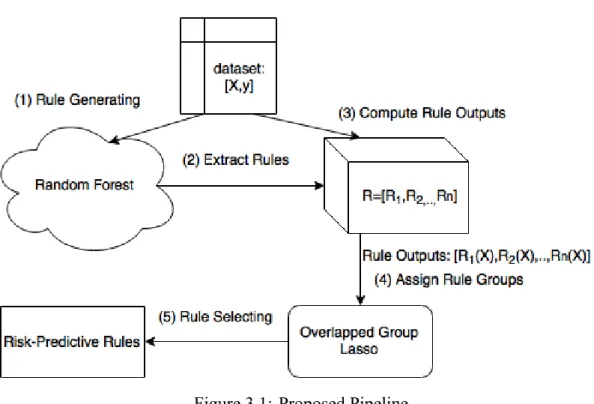
In this chapter, we describe our structured rule-based approach for risk-predictive pattern discovery by analyzing heterogeneous longitudinal complex data. It extends the existing RuleFit [6] approach to specifically address the challenge when analyzing longi-tudinal measurements, where some measurements of candidate risk factors are collected along time and hence, the corresponding features manifest as two-dimensional time-variant measurements. The essential idea of structured sparse rule discovery is to modify the Rule-Fit rule pruning procedure to replace the step with the LASSO formulation, with the over-lapped group LASSO (2.13), so that we can enforce temporal dependency structures by group regularization terms.

3.1 Problem Statement

In biomedical applications, it is often valuable but difficult to fully understand com-plex disease progression patterns. With the development of efficient high-throughput pro-filing techniques, powerful computational resources, and efficient machine learning algo-rithms, researchers hope to analyze large-scale data collected from biomolecular, clinic, and daily-life observations to seek for accurate and reproducible identification of potential risk factors that may affect and trigger disease development so that more accurate disease prognosis and effective therapeutics can be developed based on them. We propose here a structured sparse rule discovery method to identify risk-predictive patterns as compos-ite biomarkers by analyzing large-scale heterogeneous longitudinal data. The proposed method takes advantages of the existing advanced rule-based and structured sparse regu-larization methods to specifically address the critical challenges in risk-predictive pattern discovery: (1) It naturally handles the data challenges, including diverse data types and

(26)

Figure 3.1: Proposed Pipeline

potential missing values in collected measurements; (2) It incorporates the potential inter-active effects among different candidate factors by employing rule-based methods; (3) It aims to select non-redundant and significant rules as risk patterns that alleviates the po-tential overfitting problem and addresses the interpretability issues by sparse rule pruning methods; (4) Last but not least, incorporating overlap group LASSO regularization helps to take care of potential dependency structures among candidate factors and temporal de-pendency when analyzing longitudinal data.

The proposed structured spare rule discovery analysis pipeline is illustrated in fig-ure 3.1.

3.2 Data Representation

As typical in feature selection and predictive learning problems, we denote the out-come label byy, which is evaluated by a candidate feature setX= [X1,X2, . . . ,Xf], where

(27)

f is the number of candidate factors that we can collect the corresponding measurements. In biomedical studies, these candidate factors may interact with each other and influence the disease progression process. In addition, some factors may change over time when dis-ease develops. The corresponding measurements manifest as longitudinal data for these dynamic features. For clear representations, we assume that the longitudinal measurements are aligned with time points, thus we can have a subset inXin addition to static (or

base-line) features: Xˆ = [X₍₁_,₁₎, . . . ,X₍₁_,_q),X₍₂_,₁₎, . . . ,X₍₂_,_q), . . . ,X_(p_,₁₎, . . .X_(p_,_q)], where there are p dynamic features, observed atq sequential discrete time points. Hence, with both baseline and longitudinal measurements, we can represent all of them by a design matrix X= [X1, . . . ,Xf,X(1,1), . . . ,X(1,q), . . . ,X(p,1), . . .X(p,q)].

In this work, we want to derive rules as a representation of risky-predictive patterns by extending RuleFit to the integrated framework in figure 3.1 to seek for better perfor-mance on analyzing such heterogenous longitudinal data.

3.3 Structured Sparse Rule Discovery

As illustrated in figure 3.1, our rule-based approach consists of two major steps, rule generation and rule pruning.

3.3.1 Rule Generation

A rule is defined as an indicator functionR, which maps the corresponding values that a feature vectorxcan take onto a binary output by checking whether a specified condition

of the involved features is satisfied, often the observed measurements being within the specified range. A general rule function take one or more features and these features can be of different data types with binary, categorical or numerical values. We can write a rule asR(x) =I(x1∈S1)···I(xf ∈Sf), whereI(·)is an indicator function,Sf denotes the

(28)

values or continuous real values.

In the first rule generation stage, we take advantage of the existing fast random for-est algorithm [17] to generate rules by fitting decision tree models with the training data. Random forest serves as an extended decision tree model. It ensembles a large number of decision trees estimated from the training data through the bootstrap aggregating al-gorithm featured with random sampling from both subsets of samples and features. The random forest procedure helps to construct decision tree ensembles with subpopulations fully searched, and potential interactions among features are fully explored and evaluated to pick the rules with interacting features with a high likelihood as candidate risk factors when forming node splitting criteria. In this way, the full set of rules resulting from random forest can be considered informative and candidate risk-predictive patterns to describe the characteristics of the training dataset.

In each random decision tree from the derived random forest, each non-root tree node has a rule representation and hence from the root to leaf nodes, we have a hierarchy of rules involving different numbers of factors. Specifically, since the collection of trees

{T1,T2, . . . ,TM|Tm= (Vm,Em)}are derived, the corresponding path from the root in each

tree gives a ruleR(·). Hence, for a given decision treeTm, the number of generated rules

equals|Vm|−1. Such a hierarchy of derived rules naturally incorporates the potential inter-actions among features. The procedure of decision tree construction also accommodates the data issues when we need to analyze different data types of measurements with missing values.

However, due to many heuristics utilized to ensure the efficiency of random forest, a large number of weakly predictive trees and rules can be generated in this first stage. In order to better select non-redundant and significant rules, we further apply a regularized parametric model to help pruning rules to select a minimum subset of significant rules as the final risk-predictive patterns.

(29)

3.3.2 Rule Pruning

For the next rule pruning stage, we apply the overlapped group LASSO regulariza-tion to help incorporate the dependency of derived rules when pruning rules to identify significant ones as final risk-predictive patterns. Instead of directly applying the LASSO regularization as in RuleFit, which simply adopts thel1-norm penalty to produce a sparse

coefficient vector with many elements being zero, corresponding to potential weakly pre-dictive or false positive rules, we take an overlapped group LASSO regularization term that allows to enforce considering the dependency relationships among rules when pruning. It is easy to see that when we consider the dependency structure, the overlapped groups can be represented by a hyper-graph with each vertex representing a group of dependent rules and vertices connected by an edge if there are common rules within different groups. In that sense, overlapped group LASSO is a general graph-based regularization method. By incorporating such general dependency structures, we hope to achieve more stable rule discovery by selecting rules with repeatedly selected features. Due to the rule generation procedure, one feature can appear in different rules. Hence, when we incorporate such rule dependency based on common features, the group dependency relationships may lead to overlapped groups. The overlapped group LASSO formulation for rule pruning is therefore critical to consider complex and high-order interactions among original features.

In this rule pruning stage, we first integrate all the rules obtained from the rule gen-eration stage as the predictors transformed from the original features. Given a binary out-come responseY, for example, denoting the corresponding sample coming from healthy or disease subjects, we can formulate a logistic regression problem with the overlapped group LASSO regularization to select significant rules from this large number of random forest rules. Note that for each corresponding rule R(x) as the transformed predictor, it

(30)

fea-tures takes different types of values. For the pool of all the random forest rules, we can denote them by R= [R1,R2, . . . ,RN], we can now formulate the logistic regression with

overlapped group LASSO to fit high-dimensionalRagainst the outcomeY. Similar as the problem (2.13), the formulation for our rule pruning problem is

argmin_β,µ∥Y−µ·1−Rβ∥22+λ1 J

∑

j=1 √ pj∥βj∥2+λ2∥β∥1. (3.1) In the logistic regression problem, we denote the outcomeyi∈ {−1,1}, and feature

vectorxifori-th sample, then it becomes

argmin_β_,_µ 1 N N

∑

i=1 (log(1+exp(−yi(βTxi+µ)))) +λ1 J

∑

j=1 √ pj∥βj∥2+λ2∥β∥1. (3.2) Hereβjstands for a subset vector of the elements inβ, where{βn|Rnassigned to a

given group j}. The logistic loss term, _N1∑N_i=1(log(1+exp(−yi(βTxi+µ)))), is applied

to measure prediction accuracy. The l-1 norm penalty ∥β∥1, is used to minimize the size of selected rule subset. Thel-2 norm penalty with respect to each potential group of rules, is used to regularize the diversity within given groups. Here,λ₁andλ₂are two parameters to be specified to balance within the three terms, reflecting model accuracy, model com-plexity, and model internal dependency. With such a formulation, we can implement the recent optimization algorithm [24] to solve (3.1) for rule pruning.

3.3.3 How We Form Overlapped Groups

Deciding the overlapped group structure for rule pruning is critical. Based on the de-sired rule dependency structures, we propose an overlapped group hyper-graph by grouping rules based on their involvement with both baseline and dynamic features, so that the rules within the same group tend to be selected or pruned together based on their synergistic predictive power on outcome of interest.

First, we consider the rule dependency by assigning rules associated with shared fea-tures to the same groups (grouping rules by involved feafea-tures). Interacting rules (involving two or more features) are assigned to multiple groups and the number of groups will be

(31)

upbounded by the number of original features. By doing that, in addition to identifying significant rules as risk-predictive patterns, we also can have better interpretation which candidate risk factors may have larger influence on disease progression so that better prog-nosis and intervention can be designed based on that.

When considering heterogeneous longitudinal data, one of our basic assumptions is to consider the potential temporal dependency from longitudinal measurements. Denote the p-th dynamic feature’s measurement collected at theq-th time point byX_(p_,_q). In ad-dition to the rule dependency based on the feature sharing, we also consider the potential interaction of dynamic features at the aligned time points. Such rule dependency may help reveal the interactive effects on disease progression from environmental exposures for ex-ample. In this thesis, we only consider grouping rules if they involve dynamic features at the same time point but this can be extended to incorporate potential delays by setting up a time window.

Let’s denote a rule that involves both baseline and dynamic features as Rn ∼

(Xf1, . . . ,Xfa,X(p,q)1, . . . ,X(p,q)b). Here, Xfa denotes the a-th baseline feature; and X(p,q)b denotes theb-th dynamic feature. Considering the previously described rule dependency structures, there are three ways to assign rules into the same group: 1) Given baseline/static feature f fixed, group all the rules Rn∼(Xf, . . .) that involve f; 2) Given dynamic

fea-ture p, group all the rules Rn∼(Xp,q, . . .) that involve p; 3) Given time pointq for the

corresponding longitudinal measurement, group all the rulesRn∼(Xp,q, . . .)that involve

the longitudinal measurements at the same time point q for any dynamic features. We solve (3.2) for rule pruning based on such rule dependency structures modeled in the first term of (3.2).

(32)

4 EXPERIMENT RESULTS

In this chapter, we present our exploratory results by applying the structured sparse rule discovery to identify risk-predictive patterns by analyzing a large-scale dataset col-lected in a prospective T1D study. T1D have been commonly considered as complex dis-ease for subjects with pre-disposed genetic risk. However, the exact trigger(s) and disdis-ease progression processes have not been completely understood. In order to identify poten-tial genetic and early-life environmental risk factors to help predict and treat T1D, there have been several large T1D studies to collect diverse types of measurements for candidate risk factors so that systematic analysis of the collected measurements, hoping to discover risk-predictive patterns that may help predict the clinical T1D onset.

4.1 Risk-Predictive Rules for T1D

We focus on a de-identified T1D dataset with heterogeneous measurements, col-lected for binary, categorical, and numerical valued candidate factors. Some early-life en-vironmental factors, including infectious disease exposures and body-mass index (BMI), have been tracked every 3 months for the first two years for after-born children. In this study, we have 7,512 subjects and we consider whether the subject has been tested pos-itive for persistent auto-antibody tests as the disease outcome of interest. The persistent auto-antibody has been considered as the precursor of the clinical T1D onset. Hence, the early accurate prognosis may help timely intervention to delay and even prevent T1D on-set. Among 7.512 subjects in this study, there are 599 subjects with persistent confirmed positive auto-antibodies as the case population and 6,913 negative subjects as the control population. After removing redundant measurements in the original dataset, there are 97 baseline and dynamic candidate factors as features in the analysis. The details of these

(33)

features are given in a table in Appendix. Among these features, the baseline features are mostly collected from genetic tests, clinic records, daily-life behavior questionnaire, and family information. There are binary features, such as gender, and FDR (first-degree rela-tive) that indicates whether the subject has diabetic first-degree relatives (parents, siblings, etc.); categorical features (race, country, HLA (Human Leukocyte Antigen) genotype cat-egory, etc.); and numerical features (mom’s age when giving birth, number of days with a specific type of infectious disease, the age of the subject was given certain types of diet, etc.). Dynamic features include BMI and infection history of 4 categories of infectious diseases for the first 2 years of life. For example, the feature IDinf_epi_group_1_15 de-notes how many days the subject has reported (by parents) to be infected with category one infectious diseases on the 15th month.

As described in the previous chapter, we first generate rules based on orginal dataset using random forest package developed and maintained by A. Liaw,et al.[25], which nat-urally incorporates potential interactions among different features. From the adopted ran-dom forest procedure, we have generated 952 candidate rules by setting the number of trees to 250, and maximum node number for each tree as 4. The random forest training takes 9.435s. Besides, by having the assumption that there are a few features (HLA_Category, Sex, and FDR) being conjectured to be risk-predictive and have significant marginal ef-fects, we want to validate by creating additional rules just based on taking every possible value of each of those features. For example, the additional rules forFDRareFDR∈ {′1′}

and FDR ∈ {′0′}, for feature Sex are Sex ∈ {′Male′} and Sex ∈ {′Female′}, and for HLA_Category we have 12 more rules indicating whether subject belongs to particular HLA category. Thus, we have 16 more rules, finally 968 rules in total. Then, we select rules with the overlapped group LASSO formulation by pruning away weakly predictive or redundant rules. Again, the rule dependency structures are considered by grouping rules in three ways: 1) if the rules involve the same baseline feature; 2) if the rules involve

(34)

dif-ferent dynamic features at same time point(e.g bmi_03andin f_epi_group_2_03), or 3) if the rules involve the same dynamic features, even at different time points (e.g bmi_03and bmi_09).

When solving the overlapped group LASSO logistic regression, we make use of the SLEP package developed by J. Liu, et al.[26], which solves overlapped group LASSO efficiently. And grid search has been implemented to search for the optimal penalty co-efficients for for the model complexity penalty l-1 norm, and for the overlapped group penaltyl-2 norm. We search for the appropriateλ1 value between [0.001,0.05] with the

step size0.001, jointly withλ2 between[0.0001,0.005] with the step size0.0001, totally

50×50=2500setups, repeated10times each. The average running time of every 10 re-peated experiments is 1.073s. Based on the average prediction accuracy, AUC (Area Un-der Curve) of Receiver Operating Characteristic (ROC), as well as the number of non-zero coefficients obtained from the exhaustive search from neighboring grids in the parameter space, we setλ1=0.012andλ2=0.0023in (3.2).

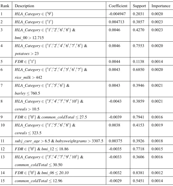
Ranked by the absolute value of the derived model coefficients in overlapped group LASSO logistic regression, the top 15 rules are provided in Table 4.1.

In this table, positive coefficient values reveal that the corresponding rules charac-terize the subpopulation that may have increased risk of developing T1D while negative coefficients characterize the protective patterns. The larger the magnitudes or absolute val-ues of the corresponding rules are; the greater the corresponding features have impact on T1D development. We also report both the Support and Important indices for the identi-fied rules. The Support index indicates how many percentages of the population are the samples that satisfy the corresponding rules. For example, if Support equals to0.5, then the corresponding rule divides the set into halves: 50% satisfying the rule and the other 50% violating the rule. The Importance index is derived based on both the corresponding model coefficient and Support, see (2.7).

(35)

Table 4.1: The Top 15 Identified Rules from OGL

Rank Description Coefficient Support Importance 1 HLA_Category∈ {′9′} -0.004947 0.2031 0.0020 2 HLA_Category∈ {′1′} 0.004713 0.3857 0.0023 3 HLA_Category∈ {′1′,′2′,′6′,′8′}& 0.0046 0.4270 0.0023

bmi_00>12.715

4 HLA_Category∈ {′1′,′2′,′4′,′6′,′7′,′8′}& 0.0046 0.7553 0.0020

potatoes>23

5 FDR∈ {′1′} 0.0044 0.1138 0.0014 6 HLA_Category∈ {′1′,′2′,′4′,′5′,′6′,′7′}& 0.0043 0.6850 0.0020

rice_milk>442

7 HLA_Category∈ {′1′,′5′,′6′}& 0.0043 0.3946 0.0021

barley≤760.5

8 HLA_Category∈ {′3′,′4′,′7′,′9′,′10′}& -0.0043 0.3859 0.0021

cereals>10.5

9 FDR∈ {′0′}&common_coldTotal≤27.5 -0.0039 0.7941 0.0016 10 HLA_Category∈ {′1′,′5′,′6′,′8′}& 0.0038 0.4153 0.0019

cereals≤323.5

11 sub j_curr_age>6.5&babysweightgrams>3307.5 0.00375 0.3926 0.0018 12 FDR∈ {′0′}&bmi_12≤18.86 -0.0035 0.7718 0.0015 13 HLA_Category∈ {′3′,′4′,′7′,′9′,′10′}& -0.0033 0.3606 0.0016

common_coldTotal≤30.50

14 FDR∈ {′0′}&bmi_06≤20.10 -0.0032 0.8381 0.0012 15 common_coldTotal≤12.96 -0.0029 0.5451 0.0014

4.2 Rule Validation via Survival Analysis

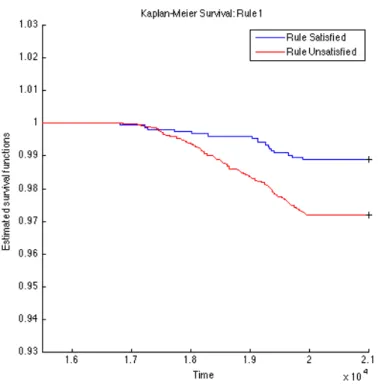
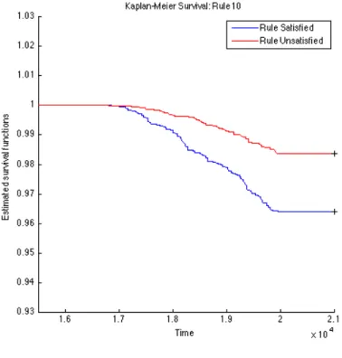
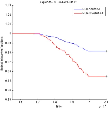
To further validate the identified rules, we carry out survival analysis on these derived rules to estimate the separability of two subpopulations distinguished by the corresponding rule. Since we have the clinical T1D diagnosed date for each subject (t1d_diag_date) for who eventually gets diagnosed with T1D clinical onset, we use these records to plot Kaplan-Meier (KM) curves for every two subpopulations partitioned by each top rule. The KM plots for the top 15 rules are given in Figures 4.1, 4.2, 4.3, 4.4, 4.5, 4.6, 4.7, 4.8, 4.9,

(36)

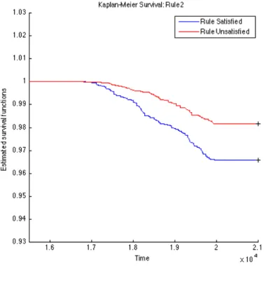
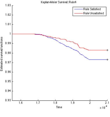
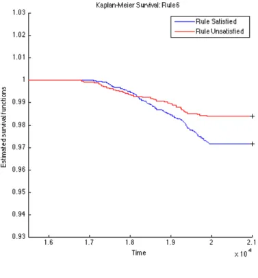
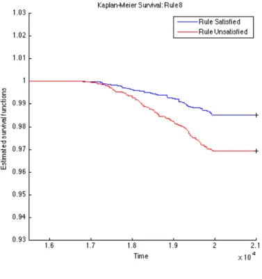
Figure 4.1: K-M: Rule01 OGL

4.10, 4.11, 4.12, 4.13, 4.14, and 4.15. The horizontal axis in the KM plot represents the aligned time since the birth of subjects, and the vertical axis represents the survival rate (the percentage of those have not been diagnosed with T1D) for a given subpopulation. The stared curves indicate the rule-satisfied subpopulations, and the cycled curves indicate the rule-violated ones.

It is clear that all these 15 top rules are risk-predictive, especially Rules 5, 9, 12, and 14. When applying log-rank tests to compare the survival distributions of subpopulations under individual rules, all the identified rules are significant withp-values<0.05as illus-trated in Table 4.2. When we check Rules 5, 9, 12, and 14, there are both risk-increasing and risk-protective patterns with their log-rank test p-values<10−9. This group of rules involve mostly the risk factors FDR, infection history, BMI and their interactions. These indeed can be found reported evidences in the T1D literature.

(37)

(38)

(39)

(40)

(41)

(42)

(43)

(44)

Table 4.2: Log-Rank Test p-values of Top 15 Rules from OGL Rules P-value of log-rank test Rules P-value of log-rank test Rule 1 2.3260e−4 Rule 9 1.2095e−11 Rule 2 2.2292e−5 Rule 10 9.7659e−8 Rule 3 5.3404e−4 Rule 11 1.8051e−3 Rule 4 1.8996e−2 Rule 12 6.8077e−10 Rule 5 <1e−16 Rule 13 5.9548e−5 Rule 6 1.8573e−3 Rule 14 2.9132e−13 Rule 7 8.8449e−8 Rule 15 4.3533e−2 Rule 8 2.4628e−5

4.3 Comparison to RuleFit with LASSO Rule Pruning

To further evaluate the rules selected from overlapped group LASSO and compare them with the results from RuleFit, we have identified top 15 rules via LASSO (without considering the overlapped group penalty termλ2=0) as in RuleFit. The corresponding

penalty parameterλ1for the model complexity penalty in (3.2) in this experiment is set to

0.03, which is also obtained from exhaustive grid search within an interval[0.0001,0.005]. The search step size was set to0.0001. We have run evaluations10times for each setup, to compare the average obtained prediction accuracy, non-zero coefficients and AUC values. The average running time of every 10 repeated experiments is 0.792s, also using SLEP package[26]. Withλ1=0.03, the logistic regression model with the same set of random

forest rules yields a decent prediction accuracy and selects a reasonable number of non-zero model coefficients. Here we list the top 15 rules from LASSO rule pruning in Table 4.3, as a comparison to the rules selected in our overlapped group LASSO framework.

(45)

Table 4.3: The Top 15 Identified Rules from LASSO

Rank Description Coefficient Support Importance 1 common_coldTotal≤27.5&FDR∈ {′0′} -0.0161 0.7940 0.0065 2 HLA_Category∈ {′3′,′4′,′7′,′9′,′10′} -0.0095 0.3606 0.0045

common_coldTotal≤30.50

3 HLA_Category∈ {′1′,′2′,′4′,′5′,′6′,′7′}& 0.0086 0.6849 0.0040

rice_milk>442

4 HLA_Category∈ {′2′,′3′,′4′,′7′,′8′,′9′,′10′}& -0.0072 0.5836 0.0036

bmi_00≤19.52

5 HLA_Category∈ {′1′,′5′,′6′,′8′}& 0.0073 0.4153 0.0036

cereals≤323.5

6 HLA_Category∈ {′1′,′2′,′6′,′8′}&bmi_00>12.715 0.0071 0.4269 0.0035 7 HLA_Category∈ {′1′,′6′,′8′}&milk_product≤525 0.0068 0.3908 0.0033 8 HLA_Category∈ {′1′,′5′,′6′}&barley≤525 0.0067 0.3946 0.0033 9 HLA_Category∈ {′2′,′3′,′4′,′5′,′7′,′9′,′10′}& -0.0067 0.5213 0.0033

bmi_12≤18.864

10 HLA_Category∈ {′2′,′3′,′4′,′7′,′9′,′10′}& -0.0066 0.5821 0.0033

in f_epi_2_21≤323.5

11 HLA_Category∈ {′2′,′3′,′4′,′5′,′7′,′8′,′9′,′10′}& -0.0054 0.6021 0.0027

rice>10.5

12 FDR∈ {′0′}&in f_epi_3_18≤0.5 -0.0052 0.8272 0.0020 13 HLA_Category∈ {′1′} 0.0048 0.3857 0.0023 14 HLA_Category∈ {′1′,′5′,′6′}&bmi_18>13.41 0.0073 0.4153 0.0036 15 HLA_Category∈ {′1′,′6′}&bmi_21>12.98 0.0042 0.3850 0.0020

As we can see from Tables 4.1 and 4.3, most selected rules by overlapped group LASSO remain consistent with those from LASSO by RuleFit. Two collections of selected rules typically involve similar features and cutoffs (e.g.HLA_Category∈ {′1′,′5′,′6′} in-deed is known as the genotypes with higher risk of developing T1D). We also have observed early-life environmental factors including BMI and infection history also have interactive effects on T1D disease development.

(46)

Figure 4.16: K-M: Rule01 LASSO

(47)

(48)

(49)

(50)

(51)

(52)

(53)

Table 4.4: Log-Rank Test p-values of Top 15 Rules from LASSO Rules P-value of log-rank test Rules P-value of log-rank test Rule 1 1.2095e−11 Rule 9 7.6264e−5 Rule 2 5.9548e−5 Rule 10 6.3691e−8 Rule 3 1.8573e−4 Rule 11 1.4774e−5 Rule 4 2.6483e−7 Rule 12 1.2430e−12 Rule 5 9.7659e−8 Rule 13 2.2292e−5 Rule 6 5.3404e−4 Rule 14 4.7007e−7 Rule 7 1.1237e−5 Rule 15 3.9779e−5 Rule 8 8.8450e−8

the rules identified with LASSO, as illustrated in Figures 4.16, 4.17, 4.18, 4.19, 4.20, 4.21, 4.22, 4.23, 4.24, 4.25, 4.26, 4.27, 4.28, 4.29, 4.30, and Table 4.4. Clearly selected rules

(54)

can serve as risk-predictive patterns for T1D development.

The rules highly ranked in LASSO approach and overlapped group LASSO ap-proach show strong consistency, as similar risk-predictive features are involved, such as HLA_Category,common_coldTotal,FDR, andBMI. Involved features also exhibit simi-lar predictive patterns,e.g., a largerBMI,HLA_Category∈ {′1′,′5′,′6′}generally indicates higher risk in our model. These discovered pattern turns out to be valid as also reported in the diabetes literature [27, 28].

Comparing to RuleFit with LASSO rule pruning, our structured sparse rule discovery with overlapped group LASSO indeed have the trend to select related factors into the top rules as we noted earlier with Rules 5, 9, 10, and 12 from overlapped group LASSO. These corresponding rules show strong statistical significance in survival analysis; and they are risk-predictive, and worthy to be selected and examined further.

In addition, with overlapped group LASSO, the rule pruning procedure may help re-duce false discovery of interacting rules. Comparing the top rules from overlapped group LASSO and LASSO, more rules involving only one factor have been ranked high in over-lapped group LASSO due to imposing the rule dependency. It naturally adjusts the contri-butions of complex interacting rules to reduce the false discovery.

Another trend can also be observed when checking the Support indices in Table 4.3. RuleFit with LASSO pruning tend to given the higher rank to the rules with Support close to 0.5 (which means preferred rules divide the whole set into halves), than those from overlapped group LASSO shown in Table 4.1. In fact, among the top 15 selected rules, the average Support for overlapped group LASSO top rules is 0.4979, with the standard deviation0.2226, and that for RuleFit rules is0.5180, with the standard deviation0.1550. Again, due to the rule dependency enforced by overlapped group LASSO, our structured sparse rule discovery does not restrict to achieving good global splitting only, but also selects the rules that may help distinguish interesting subpopulations.

(55)

Since we have observed that some important rules denoting potentially interesting subpopulations are only selected by overlapped group LASSO, we may conclude that, our overlapped group LASSO approach may help find more robust and refined subpopulations for better understanding and prediction of T1D development, compared to the original RuleFit, due to the consideration of the dependency relationships among different features and temporal measurements.

4.4 Prediction Accuracy Evaluation

Our method is not only effective in identifying top rules as disease risk-predictive patterns, but also capable of performing prediction for disease diagnosis. As a typical rule-based ensemble model, in the form of overlapped group LASSO logistic regression, the trained classifier can be applied to derive the overall risk score of a given subject.

We evaluate the prediction accuracy by AUC values. In this evaluation, in order to avoid reporting bias, we perform random sampling to obtain training and testing samples, and repeated training the model for 200 times. Each time training dataset and testing dataset are separately random sampled from original set, both with balanced outcome labels. And we want to keep the training and testing set both balanced, by which the training set is produced with balanced case and control samples, especially because the case samples have a much smaller portion (less than 10%) in the original dataset. For each evaluation experiment, we randomly sample the63%of all the case samples (since case samples take a much smaller portion) and randomly sample the same number of control samples. Then we use the model trained with the training set to make prediction on the testing set, thus obtained AUC under the current evaluation. The average AUC is obtained by repeating this process, which turns out to be0.6545.

For comparison, we also have evaluated the LASSO regularized logistic regres-sion [5] by RuleFit, which yields an average AUC value at0.6570. In addition, we plot

(56)

Figure 4.31: ROC Comparison

the ROC curves by our overlapped group LASSO model and RuleFit from one of 200 evaluation experiments, which are very close to each other. It is interesting to see that our proposed structured sparse rule discovery with overlapped group LASSO does not sacrifice too much on prediction accuracy but have the potential to incorporate more complicated dependency structures when selecting top rules as risk-predictive patterns.

We note that our structured rule discovery with overlapped group LASSO achieves slighly worse AUC compared to RuleFit-based analysis [5]. This is reasonable as we impose additional structure dependency regularizations. More critically, our method is designed to discover risk-predictive patterns. We have observed a number of rules can significantly distinguish subgroups of subjects with different trends in survival, and it is consistent with the existing findings in relevant studies. Hence, we believe our proposed structured rule-based method has the potential in helping understand disease progression. In order to comprehensively evaluate the proposed method, we will need to conduct more

(57)

experiments with well-established benchmark datasets and compare with other existing methods as similarly done in [5].

(58)

5 CONCLUSIONS

In this thesis, we have designed a structured rule-based disease risk-predictive pattern discovery framework by extending RuleFit to explicitly model potential rule dependency so that heterogeneous longitudinal data can be appropriately analyzed. Our structured spare rule discovery procedure has a few nice properties comparing to the original RuleFit. By applying overlapped group LASSO, we have the flexibility to model the dependency struc-tures among rules and feastruc-tures. This property is especially useful in a situation where we have some prior knowledge or assumptions about candidate factors.

We have obtained exploratory results by applying both RuleFit and our structured sparse rule discovery with overlapped group LASSO regularization to analyze a hetero-geneous dataset studying T1D disease progression. Our experiments have shown that its capability of identifying risk-predictive patterns for T1D development. The identified rules are consistent with the reported T1D research results. For instance, HLA genotypes have been reported as an indicator of susceptibility to T1D [29]. BMI has also been conjectured as a significant indicator of diabetes risk, especially for people at younger ages [28]. FDR is observed in our experiments as one of the dominant risk factors, which is also reported in the literature [27] as an important risk factor of T1D onset.

5.1 Future Directions

For analyzing complex disease longitudinal data, careful modeling temporal depen-dency can help reveal disease progression mechanisms and timely intervene to help delay and prevent disease onset. It is definitely an important direction for future reseach.

There can be several possible improvements for longitudinal data analysis. From our experimental results, we have not been able to figure out significant time-associated

(59)

patterns. One possible explanation may be that the temporal dependency with respect to the disease development may not be as strong as the other interactive effects identified in this specific dataset. On the other hand, only the rules with dynamic features having ob-servations at the same time points are grouped but more general temporal dependency and continuity at neighboring time points may need to be considered. For example, the feature bmi_03should be more correlated tobmi_06rather than tobmi_24. Such dependency rela-tionships may need to be integrated into the future rule-based discovery models. With the flexibility of overlapped group LASSO, we can establish a complex interaction network by adding more general dependency relationships, which may lead to more interesting pat-terns and association findings related to disease progression. We will study these potential models in our future research.