Amaral, Getulio J.A. (2004) Bootstrap and empirical
likelihood methods in statistical shape analysis. PhD
thesis, University of Nottingham.
Access from the University of Nottingham repository: http://eprints.nottingham.ac.uk/11399/1/shapetese2.pdf Copyright and reuse:
The Nottingham ePrints service makes this work by researchers of the University of Nottingham available open access under the following conditions.
· Copyright and all moral rights to the version of the paper presented here belong to the individual author(s) and/or other copyright owners.
· To the extent reasonable and practicable the material made available in Nottingham ePrints has been checked for eligibility before being made available.
· Copies of full items can be used for personal research or study, educational, or not-for-profit purposes without prior permission or charge provided that the authors, title and full bibliographic details are credited, a hyperlink and/or URL is given for the original metadata page and the content is not changed in any way.
· Quotations or similar reproductions must be sufficiently acknowledged. Please see our full end user licence at:
http://eprints.nottingham.ac.uk/end_user_agreement.pdf
A note on versions:
The version presented here may differ from the published version or from the version of record. If you wish to cite this item you are advised to consult the publisher’s version. Please see the repository url above for details on accessing the published version and note that access may require a subscription.
Bootstrap and Empirical Likelihood
Methods in Statistical Shape Analysis
by Getulio J. A. Amaral
Thesis submited to The University of Nottingham for the degree of
Doctor of Philosophy, August 2004
Contents
1 Introduction 8
1.1 Main Ideas of Shape Analysis . . . 9
1.2 Literature Review . . . 11
1.3 Mathematical Representation of Shape . . . 14
1.4 Coordinate Systems . . . 19
1.5 Definition and Simulation of Shape Distributions . . . 21
1.5.1 Complex Normal Distribution . . . 22
1.5.2 Simulation Method for the Complex Normal Distribution . . . 23
1.5.3 Complex Bingham Distribution . . . 24
1.5.4 Simulation Method for the Complex Bingham Distribution . . . 25
1.6 Confidence Regions based on Normal Approximation . . . 26
1.7 Tests for One Group of Objects . . . 29
1.7.1 Hotelling’sT2Test for a Specified Mean Shape . . . 29
1.7.2 Goodall’s Test for a Specified Mean Shape . . . 30
1.8.1 Hotelling’sT2Test to Compare the Mean Shape of Two Populations . 32
1.8.2 Goodall’s Test to Compare the Mean Shape of Two Populations . . . . 33
1.9 Scope of the Thesis and Motivation . . . 35
2 Bootstrap Confidence Regions for the Mean Shape 37 2.1 Main Ideas and Literature Review of Bootstrap Methods . . . 38
2.2 Bootstrap Confidence regions . . . 41
2.3 The Method of Fisher et al. (1996) for Axial Data . . . 44
2.4 Relationship Between Axial data and Shape Data . . . 47
2.5 Modified T-statistic for Complex Unit Vectors . . . 48
2.6 Bootstrap Confidence Regions for the Mean Shape . . . 50
2.6.1 Monte Carlo Simulation Design . . . 51
2.6.2 Mahalanobis Bootstrap Method . . . 52
2.7 Asymptotic Distribution of the Statistic T . . . 53
2.8 Practical Applications . . . 60
2.8.1 Example 2.1 . . . 60
2.8.2 Example 2.2 . . . 62
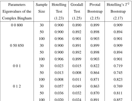
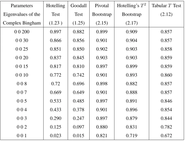
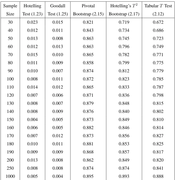
2.9 Simulation Results . . . 65
3 Bootstrap Tests in Statistical Shape Analysis 72 3.1 Bootstrap Hypothesis Testing . . . 73
3.2 Rotations Determined by Geodesics . . . 76
3.4 Asymptotic Distribution ofFB(µ) . . . 85
3.5 Some Applications . . . 95
3.6 Simulation Study . . . 95
4 Empirical Likelihood Methods in Shape Analysis 103 4.1 Main Ideas and Literature Review of Empirical Likelihood . . . 104
4.2 Definition and Properties of Empirical Likelihood . . . 107
4.3 Empirical Likelihood for a Univariate Mean . . . 110
4.4 Empirical Likelihood Regions for The Mean Direction . . . 114
4.5 Empirical Likelihood Regions for the Mean Shape . . . 117
4.6 Explicit Calculation of a set of Orthogonal Unit Vectors . . . 119
4.7 Algorithm . . . 121
4.8 Bootstrap Calibration . . . 123
4.9 Monte Carlo Simulation Study . . . 124
4.10 Simulation Results . . . 125
4.11 Graphical Representation of the EL’s Asymptotic Distribution . . . 128
4.12 Analysing Real Data . . . 128
4.13 Empirical Likelihood Tests for Several Samples . . . 131
4.14 Empirical Likelihood Hypothesis Tests in Shape Analysis . . . 133
4.15 Simulation Experiment . . . 136
4.16 A Real-data Example . . . 137
5.1 Comparing the Two Methods . . . 138
5.1.1 Bootstrap Methods . . . 139
5.1.2 Empirical Likelihood Methods . . . 139
5.1.3 Simulation Results . . . 140 5.2 Further Work . . . 144 5.2.1 A Bayesian Method . . . 144 5.2.2 Size-and-Shape . . . 145 5.2.3 Shape Variation . . . 146 A Matrix Results 149 B Order Notation 153 C The Factor 2 in(2.12) 154 D Owen’s Empirical Likelihood Program for a Vector Mean 156 References . . . 158
Abstract
The aim of this thesis is to propose bootstrap and empirical likelihood confidence regions and hypothesis tests for use in statistical shape analysis.
Bootstrap and empirical likelihood methods have some advantages when compared to con-ventional methods. In particular, they are nonparametric methods and so it is not necessary to choose a family of distribution for building confidence regions or testing hypotheses.
There has been very little work on bootstrap and empirical likelihood methods in statistical shape analysis. Only one paper (Bhattacharya and Patrangenaru, 2003) has considered boot-strap methods in statistical shape analysis, but just for constructing confidence regions. There are no published papers on the use of empirical likelihood methods in statistical shape analysis. Existing methods for building confidence regions and testing hypotheses in shape analysis have some limitations. The Hotelling and Goodall confidence regions and hypothesis tests are not appropriate for data sets with low concentration. The main reason is that these methods are designed for data with high concentration, and if this hypothesis is violated, the methods do not perform well.
On the other hand, simulation results have showed that bootstrap and empirical likelihood methods developed in this thesis are appropriate to the statistical shape analysis of low concen-trated data sets. For highly concenconcen-trated data sets all the methods show similar performance.
Theoretical aspects of bootstrap and empirical likelihood methods are also considered. Both methods are based on asymptotic results and those results are explained in this thesis. It is proved that the bootstrap methods proposed in this thesis are asymptotically pivotal.
“R”. An algorithm for computing empirical likelihood tests for several populations is also implemented in “R”.
Acnowledgements
I would like to thank my first supervisor professor Andrew Wood who gave all necessary help in all the steps of this thesis. I also would like to thank my second supervisor professor Ian Dryden who supervised this work in the first two years of the PhD.
I also would like to thank Francisco Cribari-Neto and Gauss M. Cordeiro, for their help before the PhD.
I dedicate this thesis to Severina Amaral, Jose Amaral, Vitor, Debora e Daniel. I also would like to thank god.
Notation
Symbol– Meaning Page Number
k Number of landmarks 14 m Number of dimensions 14 Y = y1,1 y1,2 .. . ... yk,1 yk,2 Configuration matrix 14
Rm m-dimensional Euclidean space 14 z0 Complex coordinates for the landmarks 15
HF Helmert matrix 15 H Helmert sub-matrix 16 w=Hz0 Helmertized configuration 16 1k Vector of ones 16 Ik k×kIdentity matrix 16 n Number of observations 16 zi=wi/||wi|| Pre-shapes 17
CSk−1 (k−1)dimensional pre-shape space 17
Ck Complex space 17 ˆ S =Pni=1ziz⋆i Complex SSP matrix 18 b λ1, . . . ,bλk−1 Eigenvalues ofSb 19 b
Notation (Cont.)
Symbol– Meaning Page Number
b
µ1, . . . ,µbk−1 Eigenvectors ofSb 19
b
µ=µb1 Sample mean shape 19
wPi =wi⋆µwb i/(w⋆iwi) Full procrustes coordinates 20
vi Tangent coordinates 21
Nk(.) k−dimensional real multivariate normal 22
CNk(., .) Complex normal 23
f(z) = πk−11|Σ|e
−(z−µ)Σ−1(z−µ)
Density of the complex normal distribution 23
f(z) =c(A)−1exp(z⋆Az) Density of the complex Bingham distribution 24
Z Random variable on the pre-shape space 24
Sv Covariance matrix of the tangent coordinates 27 F Hotelling’sT2 statistic 30
S+ Moore-Penrose inverse ofS 30
Notation (Cont.)
Symbol——- Meaning Page Number
G Goodall’s statistic 32
D Mahalanobis distance 33
H Hotelling statistic (two sample case) 33
GT Goodall statistic (two sample case) 34 u(b)={u(b)
1 , . . . , u (b)
n } Bootstrap sample 42
Rα ={ν :Tu2(ν)≤t(αB)} Bootstrap confidence region 43 Sd ddimensional real sphere 45
T(m) Statistic of Fisher et al. (1996) 45
b
m Mean polar axis 44
Rα={m:T(m)6t(αB)} Bootstrap confidence region form 46 T(µ) ModifiedT statistic in complex case 49
b
Σ Covariance matrix used inT(µ) 49
c
Mk−2 = [bµ2, . . . ,µbk−1]⋆ Matrix of the orthogonal eigenvectors ofSb 49
Notation (Cont.)
Symbol——- Meaning Page Number
F(µ) Statistic of Mahalanobis bootstrap method 52
y[j] Sample of configurations from thejthpopulation 82
z[j] Sample of pre-shapes from thejthpopulation 82
b
Σ[j] Covariance matrix for thejthgroup 84
c
Mk[j−]2 Eigenvector matrix for thejthgroup 84
FB(µb) Statistic for bootstrap hypothesis test 84 EL(m) Empirical likelihood function 107
R(ν) Empirical likelihood ratio 111
Chapter 1
Introduction
In this chapter background on shape analysis is given and notation for describing shape data is presented. Extensive accounts of shape analysis are given in the monographs by Dryden and Mardia (1998), Small (1996) and Kendall et al. (1999).
In§1.1, the main ideas of statistical shape analysis are considered. A review of the liter-ature about shape analysis is the topic of§1.2. The mathematical representation of shape and concepts such as the mean shape are reviewed in§1.3. In§1.4, coordinate systems including Procrustes coordinate systems and tangent coordinate systems are considered. Two relevant distributions, the complex normal and complex Bingham distributions, and techniques for their simulation, are studied in§1.5. How tangent coordinates can be used to obtain confidence re-gions for the mean shape via a normal approximation is reviewed in§1.6. Hypothesis tests for a single population are considered in§1.7 and for several populations in§1.8.
1.1
Main Ideas of Shape Analysis
The study of the shape of random objects has received increasing attention in several disci-plines. Advances in computer technology have made easier the capture and manipulation of images of objects. This information can be used to answer relevant questions in many dis-ciplines including biology, medicine, archeology and computer vision. Some examples of objects which have been studied are mouse vertebrae, gorilla skulls and magnetic resonance brain scans.
The concept of the shape of an object plays an essential role in this study. Statistical shape analysis is concerned with summaries and comparisons of shapes of objects.
Some steps have to be carried out in order to represent the shape of an object in a mathe-matically convenient way. A convenient approach is to place landmarks on the object, which are points for identifying special locations on the object. The numerical coordinates of the landmarks are then used to represent an object. These coordinates belong to a space which is called the landmark space. The information about the shape of an object is what is left after allowing for the effects of translation, scale and rotation (Kendall, 1984).
A new set of coordinates of an object, which will be called pre-shape coordinates, can be obtained from the coordinates of that object in the landmark space. Suitable transformations are used to remove the effects of scale and translation. The new coordinate system also represents a mapping from the landmark space to the a new space. The new space is called pre-shape space.
Two important summaries of a random sample of objects, the mean shape and the product matrix (or ssp), can be calculated using the pre-shape coordinates. The product matrix repre-sents the variation of the pre-shape coordinates and the mean shape is defined as the eigenvector associated to the largest eigenvalue of this matrix.
The shape is finally obtained by removing the rotation information in the pre-shape coordi-nates of an object. The rotation information is eliminated by rotating an object to be as close as possible to a template. The new set of coordinates of the object are inside a new space, which is called shape space.
The pre-shape and shape spaces are non-Euclidean spaces. It is therefore difficult to per-form standard statistical analyses on those spaces. To avoid the difficulties of non-Euclidean spaces it is possible to define a linear approximation to the space. A tangent space is a local linear approximation to the space at a particular point. For a given random sample of objects, the pre-shape coordinates of those objects can be projected on the tangent space at the sample mean shape. The new coordinates are called tangent coordinates.
Inference methods in shape analysis are often carried out in the tangent space. Such meth-ods work better when the data are highly concentrated. In the tangent space many commonly used procedures of standard linear multivariate analysis are available. For example, shape vari-ability can be studied by applying principal components analysis to the tangent coordinates.
There are some other possible approaches to statistical shape analysis which are not con-sidered in this thesis. Possibilities include size-and-shape analysis, reflection shape analysis and reflection size-and-shape analysis. In the size-and-shape statistical analysis of objects, the information about size is retained, and the information about rotation and location is discarded.
If one wants to perform a reflection shape study of objects, the information about reflection should be removed from the shapes of those objects. Similarly, if one wants to perform a reflection size-and-shape study of objects, the information about reflection should be removed from the size-and-shapes of those objects (see Dryden and Mardia, 1998, p. 57).
1.2
Literature Review
The first work on statistical shape analysis was done by Kendall (1977). In a later paper, Kendall (1984) gives a more complete description of the research field. Several important concepts including shape spaces, shape manifolds, Procrustes analysis and shape densities are presented and discussed in depth. He also clarifies the differences between statistical shape analysis and the theory of shape which is studied by topologists.
In Kendall (1984) a system of coordinates is also introduced; we refer to this later as Kendall’s coordinate system. One interesting fact about this system is that the location is removed by the use of a special matrix, the Helmert matrix. An important contribution of Kendall (1984) was the mathematical definition of shape, where he defines a mathematical space to represent the shape of a labelled set ofkpoints inmdimensions.
On the other hand, Bookstein (1984, 1986) presents a mathematical basis for the study of morphometrics. In this case the objects under consideration are from disciplines such as biology and medicine, and have landmarks chosen according to some biological or medical features. He also introduces what is known as Bookstein’s coordinate system, which removes the effects of translation, rotation and scale by manipulating two of the landmarks in such a way that they will be in fixed position.
When invited to comment the paper of Bookstein (1986), Kendall (1986) established the connection between their two theories. Kendall’s labelled set of k points in m dimensions corresponds to Bookstein’s landmarks. Even though they use different ways of calculating size and different coordinates systems, their ideas are quite similar in the sense of representing the shape of an object as a point in a manifold.
Procrustes analysis can be considered as a methodology for estimating for, a particular set of objects, the “optimal” scaling transformation, rotation transformation and translation transformation. The topic of Procrustes analysis was fully studied by Goodall (1991) who defined the mean shape in terms of Procrustes analysis. If the sum of squared distances between a point and the pre-shapes is minimal, then this point is said to be the mean shape.
A Gaussian model for the landmarks is also introduced by Goodall (1991). This model has a parameter for each transformation: scale, rotation and translation. Goodall (1991) also presented some algorithms to perform Procrustes analysis including an algorithm for ordinary procrutes analysis which minimizes the sum squares of the distances between two observa-tions, and a more general method using weighted least squares. He also presented an iterative algorithm for estimating the transformations with several observations. This second algorithm is called the generalized Procrustes analysis.
After applying the transformations to the pre-shapes, the Procrustes fit coordinates are obtained. The mean shape also can be obtained as the mean of those coordinates.
Goodall also defined tests for shapes in the one and two population cases. Those tests were based on statistics of F-ratio and Hotelling’sT2 type. The F-ratio test is called Goodall’s test in the literature.
Mardia and Walder (1994) considered tests for paired landmark data. They used a Gaussian model for the landmarks, where for each object there are two observations. The case of two x-rays for the same object was given as an example. They proposed a paired shape density, and they used this density to perform inference. They estimated the parameters of this distribution by maximum likelihood and they derived a likelihood ratio statistic, which can be used for testing hypotheses and for building confidence regions.
An important probabilistic model for statistical shape analysis is presented by Kent (1994). This model was the complex Bingham distribution, a complex version of the real Bingham dis-tribution. One important property of the complex Bingham distribution is complex symmetry. This complex symmetry means that a vector and any rotated version of this vector will have the same distribution. This property is useful because shape analysis can be performed while working with pre-shapes.
The complex Watson distribution, which is a special case of the complex Bingham dis-tribution, was discussed by Mardia and Dryden (1999). Maximum likelihood estimation and hypothesis testing procedures are considered, and they also illustrate how to use this distribu-tion in shape analysis.
Kent (1997) introduced a method for calculating the mean shape which is resistant to out-liers for landmark data in two dimensions. His model uses an angular central Gaussian dis-tribution for the pre-shapes. The mean shape is calculated by maximum likelihood estimation using the EM algorithm.
The geometry of the shape space is studied by Kendall (1984), Le and Kendall (1993) and Kendall et. al (1999). See also Dryden and Mardia (1998, Ch 5, 7).
1.3
Mathematical Representation of Shape
LetY be ak×mmatrix of Cartesian coordinates ofklandmarks inmdimensions which is given by Y = y1,1 . . . y1,m .. . . .. ... yk,1 . . . yk,m . (1.1)
A configuration are a set of landmarks on a particular object and the matrixY is usually called a configuration matrix.
The shape of a configuration matrix is obtained by removing the information about isotropic scaling, location and rotation. The shape space is the set of all possible shapes. The dimension of the shape space associated to objects withklandmarks inmdimension is
km−m−1−m(m−1)/2.
The term kmis the total dimension of the configuration matrix Y and we subtractm,1
andm(m−1)/2as a consequence of removing location, scale and rotation respectively (see
Dryden and Mardia, 1998, p. 56).
The landmark space is a real spaceRmwhere the Cartesian coordinates of each landmark
are represented. For example, for two dimensional objects,m= 2,and the landmark space is
R2.In this thesis, the focus is exclusively on the casem= 2.
of location, scale and rotation. When m = 2, the configuration matrix may be written as a
complex vector. Define ak×1complex vector
z0= (y1,1+iy1,2, . . . , yk,1+iyk,2)T = (z(1)0 , . . . , z(0k))T, (1.2)
which corresponds to complex coordinates for the landmarks. The superscript 0 is used to indicate that the configuration retains the effects of location, scale and rotation. The details of each transformation in the casem= 2will be given below.
The first step is to remove location. This can be done in various ways, depending on the coordinate system. Kendall’s coordinates will be used here. Details about the Helmert matrix and Helmert sub-matrix are needed for Kendall’s coordinate system. The Helmert sub-matrix provides a particular linear transformation which removes location by pre-multiplyingz0(see Small, 1996, p. 130, and Dryden and Mardia, 1998, p. 34).
The full Helmert matrixHF is ak×korthogonal matrix whose first row has all elements
equal to1/√k,and has rowj+ 1forj≥1given by
(hj, . . . , hj,−jhj,0, . . . ,0), hj =−{j(j+ 1)}−1/2,
withj= 1, . . . , k−1, where the number of zeros elements in the rowj+1is equal tok−j−1.
HF = 1/√5 1/√5 1/√5 1/√5 1/√5 −1/√2 1/√2 0 0 0 −1/√6 −1/√6 2/√6 0 0 −1/√12 −1/√12 −1/√12 3/√12 0 −1/√20 −1/√20 −1/√20 −1/√20 4/√20 .
It can be shown by direct calculation that the Helmert matrixHF is an orthogonal matrix.
The location of the complex configurationz0 is removed by multiplying it by the(k−1)×k
Helmert sub matrix, which is the Helmert matrixHF with the first row removed. The Helmert sub-matrix will be calledH.The Helmertized configuration is given by
w=Hz0. (1.3)
A configuration is said to be centered if 1Tkz0 = 0 where 1k is a k×1 vector of ones.
Helmertized configurations are connected to the centered configurations by the following prop-erty of the Helmert matrix (see Dryden and Mardia, 1998, p. 54):
HTH =Ik−
1
k1k1 T k,
whereIk is ak×kidentity matrix and1k is ak×1vector of ones. Moreover, sinceHF is
orthogonal, it follows thatHTH =I
k−1.Thus, if the(k×1)vectorz0 = (z0(1), . . . , z0(k))T is
a complex configuration, then
(Ik−
1
k1k1 T
wherez¯0 = k−1Pki=1z(0i).Therefore, sincez0 −z¯01k is a centered configuration, it means
that the centered configurations are equal to the Helmertized configurations multiplied byHT.
So it always possible to obtain the Helmertized configurations from the centered configurations and vice versa.
The scale can be removed from the Helmertized configurationwusing
z=w/√w⋆w=Hz0/p(Hz0)⋆Hz0, (1.4)
wherew⋆ is the complex conjugate transpose ofw. The vectorzis called the pre-shape of the complex configurationz0.This name was coined by Kendall (1984). Note that a pre-shape is a shape with rotation information retained.
The concept of pre-shape space will be reviewed because it plays an important role (see Dryden and Mardia, 1998, p. 59 and Small, 1996, p. 9). The pre-shape space is the space of all possiblek−1complex vectors that do not have translation and scale information. Thus the
pre-shape space is a unity complex hypersphere in(k−1)−dimensional complex dimensions;
i.e.
CSk−1 ={z∈Ck−1 :z⋆z= 1}, (1.5)
whereCk−1is(k−1)−dimensional complex space.
The shape space can be thought of as the pshape space with rotation information re-moved. The rotation information in the pre-shape vectorzcan be eliminated by defining the equivalence class
[z] ={eiθz:θ∈[0,2π)}, (1.6)
where [z]is identified with any of its rotated versions. Kendall (1984) notes that the shape
space whenm= 2is the complex projective spaceCPk−2,the space of complex lines passing
thought the origin.
An important problem of shape analysis is to estimate the average shape of a random sam-ple of configurations. Considerz0
1, . . . , zn0as a random sample of complex configurations from
a population of objectsΠ,where eachzi0is defined by(1.2).
Let z1, . . . , zn be the pre-shapes of z10, . . . , zn0, where zi is defined via (1.4) and zi ∈ CSk−1.The full Procrustes mean shapeµbcan be found as the eigenvector corresponding to
the largest eigenvalue of the complex sum of squares and product (SSP) matrix which is defined by (see Kent, 1994) ˆ S = n X i=1 zizi⋆.
Since the complex matrix Sbsatisfies the condition thatSb= Sb⋆, this matrix is Hermitian. Provided that the underlying distribution of the pre-shapes has a density with respect to the uniform distribution on the pre-shape sphere andn≥k−1,as opposed to being concentrated
on a subspace, thenSbhas full rank with probability 1. So, applying the spectral decomposition theorem for Hermitian matrices which is given in Theorem(A.1)in appendix A ,Sbis written as ˆ S= k−1 X j=1 b λjµbjµb⋆j, (1.7)
where bλ1 > bλ2. . . > bλk−1 > 0 are the eigenvalues, and µb1, . . . ,µbk−1 the corresponding
eigenvectors ofS.ˆ
Provided thatbλ1 >λb2, . . . ,which will usually be the case in practice, the mean shapeµbis
well defined and is given by
b
µ=µb1. (1.8)
1.4
Coordinate Systems
In statistical shape analysis there several coordinate systems in common use. Each coordinate system is useful for some aspects of the analysis. Two coordinate systems will be considered here: full Procrustes coordinates and the tangent coordinates.
Procrustes analysis is a technique to match two objects up. When two or more objects are considered, they may have different rotations, translations and scales. So the technique of Procrustes analysis is used to match one object into the other. It is done using the pre-shapes of those objects since the pre-shapes have the same translation and scale.
For a given sample of pre-shapes, Procrustes analysis is performed by fitting the pre-shape of each object onto the mean shape. The new coordinates are called Procrustes fits or Procrustes coordinates and they will be defined below.
Let z1, . . . , zn be a random sample of pre-shapes, and also letw1, . . . , wn be a random
sample of Helmertized configurations.
The configurations have an arbitrary rotation (see Dryden and Mardia, 1998, pp. 44-45). Thus, before proceeding with statistical shape analysis, it is necessary to rotate all the
config-urations in such way that they will be as close as possible of the sample mean shape. This is done by calculating
wiP =w⋆ibµwi/(wi⋆wi), i= 1, . . . , n. (1.9)
ThuswP1, . . . , wPn are called the full Procrustes fits or full Procrustes coordinates.
Since the pre-shapes can be written aszi=wi/||wi||,where eachziis defined in(1.4)and
||wi||=pw⋆iwi, the Procrustes coordinates can also be calculated from
wPi =zi⋆µzb i, i= 1, . . . , n.
Another useful system of coordinates is the tangent space coordinates. The concepts of tangent vectors and tangent space need to be presented before the definition of tangent coordi-nates (see Small, 1996, pp. 42-46). The tangent space of the shape spaceCPk−2at the point z
is the vector space of all the tangent vectors toCPk−2at the pointz. When performing tangent
space inference, the tangent space at the sample mean pre-shape is often used.
The analysis of shape variability may be carried out in the tangent space. This space is a linearized version of the shape space. One of the main advantages of the tangent space is that standard multivariate techniques can be used directly.
There are several different types of tangent space coordinates. Here we use the partial Procrustes tangent coordinates, which are given by
ti=eiθb[Ik−1−µbµb⋆]zi, i= 1, . . . , n, (1.10)
Suppose thatz1, . . . , znis a random sample of pre-shapes andt1, . . . , tntheir tangent
co-ordinates, where eachziandtiare calculated using(1.4)and(1.10),respectively. Letvi be a
2k−2vector which is obtained by stacking the real and imaginary coordinates of eachti. If
ti =xi+iyi, this operation is represented bycvecwhere
vi=cvec(ti) = (xTi , yiT)T, (1.11)
wherexi = Re(ti) is the real part ofti andyi = Im(ti)is the imaginary part ofti.If the
number of landmarks isk, a pre-shape vectorzi has dimension(k−1)and its corresponding
vector of tangent coordinatesvi,whereviis given in(1.11),has dimension(2k−2).
Standard multivariate methods can be applied to the real tangent coordinates vi. When
the data are highly concentrated, methods based on the multivariate normal distribution can be applied for the real tangent coordinatesvi (see Dryden and Mardia, 1998, p. 151). Some of
these methods will be considered in the next sections.
1.5
Definition and Simulation of Shape Distributions
This section aims to review two distributions relevant to shape analysis: the complex normal distribution and the complex Bingham distribution. Methods for simulating these distributions are also discussed. The complex Bingham distribution is suitable for modelling pre-shapes and shapes and it will be used to evaluate the computer intensive methods of the next chapters.
1.5.1 Complex Normal Distribution
Since the multivariate complex normal and multivariate normal distribution are related, it is necessary to review the multivariate normal distribution.
The multivariate normal distribution is an extension of the univariate normal distribution to
(2k−2)variables (see Mardia et. al, 1979, p. 37), where the number of variables is chosen as
(2k−2)to make a connection with the shape context. The probability density function (pdf)
of the multivariate normal of a(2k−2)real vectorxis given by
f(x|µ, V) = 1
(2π)(k−1)|V|
−1/2exp
{−12(x−µ)TV−1(x−µ)}, (1.12) whereV is(2k−2)×(2k−2)positive definite matrix,|V|= detV,andµis a(2k−2)real
vector.
A multivariate complex normal distribution can be represented as a real multivariate normal distribution (see Dryden and Mardia, 1998, p. 112). To clarify this relationship, consider the
(k−1)complex vectorz= (z1, . . . , zk−1)T and the(2k−2)real vector
v= (xT, yT)T = (x1, . . . , xk−1, y1, . . . , yk−1)T, (1.13)
wherexj =Re{zj}is the real part ofzjandyj =Im{zj}is the imaginary part ofzj.Suppose
that v∼N2k−2 (µT1, µT2)T, 1 2 Σ1 −Σ2 Σ2 Σ1 , (1.14)
whereN2k−2(µ,Σ)denotes a2k−2multivariate normal distribution with mean vectorµand
covariance matrixΣ,Σ2 =−ΣT2 is skew-symmetric andΣ1is symmetric positive definite.
The distribution of the complex vector z is known as the complex normal distribution, which is denoted byCNk−1(µ,Σ), whereν =µ1+iµ2andΣ = Σ1+iΣ2,(see Dryden and
Mardia, 1998, p. 112). The pdf ofzis given by
f(z) = 1
πk−1|Σ|e
−(z−µ)⋆Σ−1(z−µ)
. (1.15)
In the real case, it is well-known that the quadratic form (x−µ)TV−1(x−µ)in(1.12)
has aχ2
2k−2distribution. However, in the complex case, it is2(z−ν)⋆Σ−1(z−ν)which has
aχ2
2k−2distribution. The need for this factor2is explained in appendix C.
1.5.2 Simulation Method for the Complex Normal Distribution
Consider the problem of generating a vectorz which has a complex normal distribution with complex meanµand Hemitian covariance matrixΣ.
The complex Gaussian vectorzwill be represented as a real multivariate Gaussian vector
v;see(1.14).Thenvis simulated using a standard method (See Bratley et al, 1983, p. 152),
andzis obtained fromvby the inverse operation tocvecin(1.11).
The procedure to generate a2(k−1)real Gaussian vectorvin(1.14)is defined as follows.
LetAbe a(2k−2)×(2k−2)upper triangular matrix such that
ATA= 1 2 Σ1 −Σ2 Σ2 Σ1 ,
Letu ∼ N2k−2(02k−2, I2k−2),where02k−2 is a2k−2vector of0.Then the vectorv is
given by
v= (µT1, µT2)T +ATu,
whereµ1 andµ2are real(k−1)vectors, andzis obtained by applying the inverse operation
to(1.11)tov.
So thek−1-dimensional vectorzhas complex normal distribution with mean vectorµ=
µ1+iµ2 and covariance matrixΣ = Σ1+iΣ2.
1.5.3 Complex Bingham Distribution
One of the most useful distributions for two dimensional landmark datasets is the complex Bingham distribution. A detailed account of this distribution is given by Kent (1994). This is a distribution on the space of complex unit vectors, or equivalently, the complex unit sphere.
Ifz is a random complex unit vector with complex Bingham distribution, the pdf ofz is given by
f(z) =c(A)−1exp(z⋆Az), z∈CSk−1, (1.16)
whereAis a(k−1)×(k−1)Hermitian matrix andc(A)is a normalizing constant. IfA=I,
f(z)becomes a uniform distribution onCSk−1,due to the constraintz⋆z= 1.
The complex Bingham distribution has the property of complex symmetry, which means thatzande(iθ)z,whereθ∈[0,2π),have the same distribution (see Kent, 1994, p. 290). This is an important reason for using this distribution as a plausible model for the analysis of landmark
data in two dimensions, since a shape distribution should respect the definition of shape given in (1.6).
1.5.4 Simulation Method for the Complex Bingham Distribution
To simulate from the complex Bingham distribution, which is defined in (1.16), one of the methods proposed by Er (1998) is reviewed. Initially,(k−2)truncated exponentials are
gen-erated subject to a linear constraint, and then these random variables are expressed in polar coordinates to deliver a complex Bingham distribution.
LetT E(λ)denote theexp(λ)distribution conditioned to lie in[0,1]. A simple algorithm
for simulating theT E(λ)distribution is as follows.
It should be noted thatλhere is the rate.
Algorithm 1.1. Simulation ofT E(λ)
1 - Simulate a uniform random variableu∈[0,1].
2 - CalculateX =−(1/λ) log(1−u(1−exp−λ)).
The method for simulating the complex Bingham distribution uses(k−2)truncated
ex-ponentials to generate a (k−1)vector with a complex Bingham distribution. Suppose the
eigenvalues ofAare˜λ1 ≤. . .≤λ˜k−2<˜λk−1,and writeλj = ˜λk−1−λ˜j, j = 1, . . . , k−2.
The input is a(k−2)-vector
˜
λ= (λ1, . . . , λk−2). (1.17)
1 - Generate S = (S1, S2, . . . , Sk−2)T where Sj ∼ T E(λj) are independent random
variables simulated using Algorithm1.1.
2 - IfPkj=1−2Sj <1, writeSk−1 = 1−Pkj=1−2Sj. Otherwise, return to step 1.
3 - Generate independent anglesθj ∼U[0,2π), j= 1, . . . , k−1.
4 - Calculatezj =Sj1/2exp(iθj),j = 1, . . . ,(k−1).
The algorithm delivers a(k−1)vectorz= (z1, . . . , zk−1)T,which has a complex Bingham
distribution. Note that(Sj1/2, θj)are essentially polar coordinates for complex numberzj.
If the parameter matrixAhas spectral decompositionA = ΓΛΓ⋆ (see appendix A), with
Γ6=Ik−1,thenΓzrather thanzshould be returned.
1.6
Confidence Regions based on Normal Approximation
The tangent coordinates can be used for building confidence regions based on a normal ap-proximation. First, it is necessary to study the variability on the tangent space. This variability can be studied using the method of principal components. The principal component method can also be used for building approximate normal-based confidence regions on the landmark space. These issues will be considered in this section.
Consider a random sample of complex configurations z0
1, . . . , zn0,where z0i was defined
in(1.2).Suppose thatv1, . . . , vnare the tangent coordinates of those complex configurations,
wherevi is defined in(1.11).The variability in the tangent space is measured by the sample
Sv = 1 n n X i=1 (vi−¯v)(vi−v¯)T, (1.18) wherev¯=Pni=1vi/n.
The method of principal components can be used to summarize the variability of a random vector (see Mardia, et. al, 1979, p. 213). The idea of the principal component method is to reduce the dimension of the sample by focusing on the most important directions of variability. In the shape analysis context, the idea is to apply the principal component method to the sample covariance matrix of the tangent coordinates, to obtain the first few principal components and to project those components back to the landmark space (see Dryden and Mardia, 1998, pp. 47-51).
The matrixSvcan be written in terms of the spectral representation
Sv = p
X
i=1
φiuiuTi , (1.19)
wherep=min(2k−4, n−1)is the total number of principal components ,φ1 ≥. . . ≥φp
are eigenvalues andu1, . . . , upthe eigenvectors ofSv (see Mardia et al, 1979, pp. 469).
The shape variability on the tangent space is studied using the principal components via the equations
v= ¯v+cpφjuj, j = 1, . . . , p, (1.20)
wherecis a constant,v¯is defined below(1.18)andφj anduj were defined below (1.19).
Insight can be gained by giving different values to the constant c.Under the assumption that the tangent coordinates follow a multivariate normal distribution, it can be shown thatcis
approximatelyN(0,1)(see Dryden and Mardia, 1998, p. 49). On this basis, a plausible range
of values for c is[−3,3].
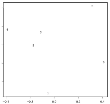
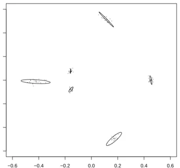
The principal components method can also be used for building confidence regions based on a normal approximation (NA). The idea of using principal components for building a con-fidence region for the mean shape is particularly appealing when the observations on the land-mark space for each landland-mark follow a bivariate normal distribution. The assumption of nor-mality is more plausible for highly concentrated data.
The confidence regions obtained by normal approximation, referred to below as NA confi-dence regions, are calculated using the principal components for tangent coordinates. The NA method uses those principal component, conveniently relocated by replacingv¯by the mean
shapeµb (see(1.8)) in (1.20), to obtain the coordinates of the objects in the landmark space. Only the first and the second principal components are used since with those components it is possible to construct an ellipse for each landmark and represent it in a2Dplot. The axes of
this ellipse are determined by the eigenvectors, and the relative scale along each axes is deter-mined by the eigenvalues, corresponding to the two leading principal components. Thus NA confidence regions can be represented graphically by a plot of
b
µ+cpφ1u1andµb+c
p
φ2u2 (1.21)
where usuallyc∈ (−3,3),µbis given in(1.8)andφj anduj were defined below (1.19). See
1.7
Tests for One Group of Objects
We consider two methods in current use for testing if the mean shape is equal to a particular value. One is the one-sample Hotelling’sT2test and the other is the one-sample Goodall test. The first one is less restrictive than the second but more complex. The Goodall test assumes the joint distribution on the landmark space is complex normal and isotropic (see Dryden and Mardia, 1998, p. 160), which means that the variance for each landmark is the same. On the other hand, the Hotelling’sT2test assumes normality for the observations on the tangent space and isotropy is not assumed.
1.7.1 Hotelling’sT2 Test for a Specified Mean Shape
Consider the assumptions of the one sample Hotelling’sT2 test. Letz01, . . . , z0nbe a random sample of complex configurations,z1, . . . , znbe the pre-shapes of those configurations, where ziis calculated from(1.4),and letµbbe the mean shape of this sample, calculated using(1.8).
Letv1, . . . , vn be the partial Procrustes tangent coordinates of those pre-shapes, wherevi is
obtained from (1.11). Recalling the tangent sample meanv¯ and tangent sample covariance
matrixSvfrom(1.18), suppose that thevihave a multivariate normal distribution.
The aim of the Hotelling’sT2test is to evaluate the hypotheses
H0 : [µ] = [µ0]versus H1 : [µ]unrestricted,
where [µ0] is a pre-specified value for the mean shape. Here [µ] can be thought of as an
are given by
γ0= (I2k−2−cvec(ˆµ)cvec(ˆµT))cvec(µP0/||µP0||), (1.22)
where cvec(.) was defined in(1.11), andµP
0 is the procrustes fit ofµ0, which is calculated
using(1.9).The statistic used for this test is given by
F = (n−M)
M (¯v−γ0) TS+
v (¯v−γ0), (1.23)
whereγ0 is given in(1.22),Sv+ is the Moore-Penrose generalized inverse (see appendix (A))
ofSv,andM is the dimension of the tangent space and calculated as2k−4.
This statistic has anFM,n−M distribution underH0. The hypothesisH0 is rejected at the
levelαifF ≥F(M, n−M, α), whereF(M, n−M, α)is the quantile of the F distribuition
with numeratorMand denominatorn−Mfor theαsignificance level.
1.7.2 Goodall’s Test for a Specified Mean Shape
The situation is similar to Hotelling’s test but isotropy is assumed. Letz1, . . . , zn a random
sample of pre-shapes, where eachzi is given by(1.4).Also consider the tangent coordinates
v1, . . . , vnof those pre-shapes, wherevi is defined in(1.11).
Goodall’s test has the assumption that the tangent coordinates follow an isotropic normal model. So thevi have a multivariate normal distribution with mean vectorµand covariance
matrixΣ =σ2I2k,whereσ2 is a constant andI2kis the2k×2kidentity matrix (see Goodall,
1991, p. 314 and Dryden and Mardia, 1998, p. 160).
H0 : [µ] = [µ0] versus H1 : [µ]6= [µ0].
The Goodall test is based on the squared Procrustes distances. For the pre-shapeszi and zj,defined in(1.4),this distance is given by
dF2(zi, zj) = 1−zi⋆zjzj⋆zi, (1.24)
fori= 1, . . . , n(see Dryden and Mardia, 1998, p. 41).
Ifµb, the estimator ofµ, is close toµ,andσ is small, the approximate analysis of variance (ANOVA) is given by n X i=1 d2F(zi, µ) = n X i=1 d2F(zi,µb) +nd2F(µ,µb),
(see Dryden and Mardia, 1998, p. 160).
Under the null hypothesis H0, the distribution of the squared Procrustes distances are
ap-proximately chi-squared distributions, e. g.,
d2F(zi, µ0)∼τ02χ2M,
whereτ0 =σ/||µ0||andM = 2k−4.The proof of this result is derived using a Taylor series
expansion (see Dryden and Mardia, 1998, p. 161).
Using this result and the additive property of independent chi-squared distributions,
n
X
i=1
Thus the test statistic (see Dryden and Mardia, 1998, pp. 160-161) is given by G= (n−1)n d 2 F(µ0,µb) Pn i=1d2F(xi,µb) ∼FM,(n−1)M. (1.25)
1.8
Tests for Several Populations
Two tests to compare the mean shape of two populations are considered in this section. The first one is the Goodall test and the second is the Hotelling’s T2. Those tests are extended versions of the tests of§1.7.
1.8.1 Hotelling’sT2 Test to Compare the Mean Shape of Two Populations
The test is used to compare the mean of two populations on the pre-shape space. However, the quantities being used are from the tangent space. This aspect will be clarified after the definitions of these quantities.
Consider an independent identically distributed (IID) random samplez10j, . . . , zn0jjof com-plex configurations from the populationΠ[j],wherej= 1,2. Letz1j, . . . , znjjandv1j, . . . , vnjj
be the pre-shapes and the tangent coordinates ofz0
1j, . . . , zn0jj, wherezljandvljare calculated
fromz0ljusing(1.4)and(1.10).
The main assumptions of Hotelling’sT2test are normality and homogeneity across
popula-tions of covariances matrices for the tangent coordinates. Suppose that the tangent coordinates
v1j, . . . , vnjj for populationjare IID, and approximately normally distributed with meanµ
[j]
and common covariance matrixV.
H0 : [µ[1]] = [µ[2]] = [µ]versus H1 : [µ[1]], [µ[2]]unrestricted, (1.26)
where[µ]is the common mean shape.
Let µb[j] and Vb[j] be the estimated mean and estimated covariance matrix of the tangent
coordinatesv1j, . . . , vnjj,whereVb
[j]has divisorn
j.The Mahalanobis distance betweenbµ[1]
andµb[2]is given by
D= (bµ[1]−µb[2])TVb+(µb[1]−µb[2]),
whereVb = (n1Vb[1]+n2Vb[2])/(n1+n2−2),andVb+is the Moore-Penrose generalized inverse
ofV ,b which is defined in (A.3) in appendixA.
The test statistic is
H= n1n2(n1+n2−M−1) (n1+n2)(n1+n2−2)M
D (1.27)
which, underH0,has anFM,n1+n2−M−1 distribution, whereM = 2k−4(see Dryden and
Mardia, 1998, p. 154).
1.8.2 Goodall’s Test to Compare the Mean Shape of Two Populations
Goodall’s test assumes that the tangent coordinates have a jointly Gaussian distribution with an isotropic covariance matrix.
It should be noted that these assumptions are reasonable for data sets for which the vari-ances of each landmark are small and similar. The hypotheses are
H0 : [µ[1]] = [µ[2]] = [µ]versus H1 : [µ[1]], [µ[2]]unrestricted, (1.28)
where[µ]is the common mean.
To obtain the statistic of the test some results about the distribution of some Procrustes distances need to be used. These results are valid underH0 and withσ small. Therefore this
test is appropriate for highly concentrated data. Set
τ0 =σ/||µ0||,
where||µ0||=
p
µ⋆
0µ0.
The distribution of the Procrustes distances for each sample is given by
n
X
i=1
d2F(zi1,bµ[1])∼τ02χ2(n1−1)M, (1.29)
whered2F(., .)is defined in(1.24),and
n
X
i=1
d2F(zi2,bµ[2])∼τ02χ2(n2−1)M. (1.30)
The Procrustes distance between the sample mean of the groups is given by
n X i=1 d2F(bµ[1],µb[2])∼τ02 µ 1 n1 + 1 n2 ¶ χ2M. (1.31)
Thus, underH0and withσsmall, using (1.29), (1.30) and (1.31), the statistic
GT = n1+n2−2 (n1)−1+ (n2)−1 d2F(µb[1],µb[2]) Pn i=1d2F(zi1,bµ[1]) +Pni=1d2F(zi2,µb[2]) (1.32)
has the approximate distribution FM,(n1+n2−2)M (see Dryden and Mardia, 1998, p. 162),
whereM = 2k−4as before.
.
1.9
Scope of the Thesis and Motivation
The contents of the following chapters are explained below. Some motivations for the thesis are given at the end of this section.
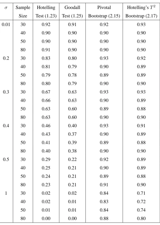
Chapter 2 explains how the bootstrap method of Fisher et al. (1996) for building confi-dence regions for directional data can be adapted to the shape context. It is proved that the distribution of the test statistic is asymptoticallyχ2 under the null hypothesis and is therefore asymptotically pivotal. The coverage accuracy of the bootstrap confidence region is compared numerically to Goodall and Hotelling confidence regions.
Chapter 3 introduces a bootstrap hypothesis test of a common mean shape across several populations. A proof that the statistic test is asymptotically pivotal under the null hypothesis is presented. This bootstrap test is compared to corresponding tests based on Goodall and Hotelling statistics using numerical simulation.
Chapter 4 presents both empirical likelihood confidence regions and hypothesis tests for shape data. First, it is explained how the empirical likelihood confidence regions of Fisher et. al. (1996) can be constructed in the shape context. Subsequently, an empirical likelihood hypothesis test of a common mean shape is introduced. Numerical simulations are carried out in order to compare these empirical likelihood methods to Goodall and Hotelling procedures.
empirical likelihood methods are compared, and numerical and methodological aspects are considered. How to apply the methods of this thesis in other areas of shape analysis is also discussed briefly.
The Goodall and Hotelling’sT2 tests work well under the assumption of high concentra-tion, but they perform poorly when applied to data with low concentration. Even though the majority of shape datasets are highly concentrated, some datasets have low concentration. This provides motivation for using bootstrap and empirical likelihood methods in the shape analysis context, because they work well when applied to data having either high or low concentration. A second motivation is that bootstrap and empirical likelihood methods are nonparametric and only require weak assumptions about the underlying population.
Chapter 2
Bootstrap Confidence Regions for the
Mean Shape
The aim of this chapter is to explain how the bootstrap confidence regions developed by Fisher et al. (1996) can be extended to the statistical shape analysis context. Fisher et al. (1996) proposed some bootstrap methods for building confidence regions for directional and axial data. Since there is a relationship between axial data and shape data for landmarks in two dimensions, it is possible to adapt bootstrap methods for axial data to shape data.
The sections are organized as follows. The main ideas and a literature review of the boot-strap are given in§2.1. Methodology for constructing bootstrap confidence regions is reviewed in§2.2. In §2.3 the bootstrap method of Fisher et al. (1996) for axial data is reviewed. The connection between axial and shape data is explained in§2.4. In§2.5 an asymptotically pivotal statistic for a sample ofncomplex unit vectors is described. The bootstrap method for shape data, which is adapted from the bootstrap method for axial data, is explained in§2.6. In§2.7
the asymptotic distribution of the statistic we propose for shape data is derived. Some practical examples are considered in§2.8. In§2.9 some simulation experiments are performed in order to compare the bootstrap method for shape data with Goodall and Hotelling procedures.
2.1
Main Ideas and Literature Review of Bootstrap Methods
The main ideas about the bootstrap were introduced by Efron (1979). Efron (1979) presented the bootstrap as a more general method than the Quenouille-Tukey jackknife. According to Efron (1979), the jackknife can be considered as a linear expansion method for approximating the bootstrap.Before explaining the bootstrap idea it is worth explaining what a functional is. A func-tional is a function of a function. Thus the notation
ν(F) where ν:{space of distribution functions} →Rd (2.1)
means thatν(F)is function of the distribution functionF. For example, ifν(F)is the variance
function andF is the distribution function of the normal distributionN(µ, σ2), thenν(F) is equal toσ2.
To explain Efron’s (1979) original idea, letu = {u1, . . . , un} be a random sample from
a distribution with cumulative distribution function (CDF)F. Suppose that we are interested in an unknown parameterν = ν(F),and let Fbn(u) = n−1Pni=1I(ui ≤ u),whereI(.) is
the indicator function, denote the empirical distribution function based on the sampleu.The
distribution ofνbby drawing resamples randomly with replacement from the original sample
u,the main point being that the resampling distribution can be estimated to arbitrary accuracy
using computer simulation.
Efron (1979) also considered the parametric bootstrap. The bootstrap mentioned above is nonparametric. But it is possible to define a parametric bootstrap by estimating F by its parametric maximum likelihood estimator. For example, it is possible to assume thatF has a normal or any other particular distribution. The resamples with replacement will be not gen-erated from the sample but from the parametric distributionF, with the parameters estimated from the sample.
Asymptotic properties of bootstrap methods can be examined using Edgeworth expansions. A seminal paper was Singh (1981). Singh (1981) showed theoretically that the bootstrap ap-proximation for a distribution function of a sample mean is generally more accurate than the limiting normal distribution function approximation. For the case of quantiles he showed that the bootstrap approximation is as good as the normal approximation.
Bickel and Freedman (1981) showed some examples where the bootstrap approximation does not work so well. They conclude that for the majority of models with many parameters the bootstrap typically fails.
Hall (1992) presents very detailed information about bootstrap methods and Edgeworth expansions. Among other things, he explained the advantage of using an asymptotically pivotal statistic for bootstrapping (see Hall, 1992, pp. 83-91). A statistic is asymptotically pivotal if its limit distribution does not depend on unknown quantities (see Hall, 1992, p. 14). Considering an asymptotically normally distributed statistic T, Hall (1992) showed that bootstrappingT
reduces the error in the distribution function approximation from ordern−1/2 to order n−1. However, if an asymptotically non-pivotal statistic is used the error does not reduce, its size is
n−1/2.Hall’s (1992) discussion is very relevant for the bootstrap methods of this and the next chapter.
A number of authors have discussed bootstrap methods for confidence regions. A vari-ety of methods for constructing nonparametric confidence intervals were introduced in Efron (1982). Some other important results can be found in Abramovitch and Singh (1985), Beran (1988), Hinkley (1988), Fisher and Hall (1990), and Hall and Wilson (1990), Hall (1988a), Hall (1988b) and Hall (1990).
Hall (1988a) compares five bootstrap confidence intervals. They come from both para-metric and nonparapara-metric contexts. Among the five methods, percentile-t and accelerated bias correction were identified as being superior. He also found that there is not a conclusive differ-ence between the two methods: they achieve similar accuracy in both theoretical and numerical performance. Hall’s (1988a) theoretical comparisons were made using Edgeworth expansions. Asymptotic results clearly demonstrate the advantage of bootstrapping an asymptotically pivotal statistic for both hypotheses tests and confidence regions. Some papers supporting the use of pivotal statistics are Beran (1987), Liu and Sing (1987), Hall (1986), Hall (1988a) and Fisher et. al. (1996).
Bootstrap methods can be applied in many different areas of statistics, including general-ized linear models, time series, sample surveys and statistical quality control, to name a few. These applications are covered in textbooks such as Efron and Tibshirani (1983), Davison and Hinkley (1997) and Chernick (1996).
In the directional data context, several papers have considered the use of the bootstrap for constructing confidence regions for the mean direction or mean axis of a population. See Ducharme et al. (1985), Fisher and Hall (1989) and Fisher et al. (1996). We now describe the developments in these papers in more detail.
Ducharme et al. (1985) developed a bootstrap method for directional data analysis for building confidence cones. They reviewed some parametric methods which are based on the assumption that the underlying distribution is a Fisher distribution. They presented a new bootstrap method which makes assumptions about the underlying distribution. In particular, the method of Ducharne et al. (1985) is not asymptotically pivotal except in relatively special circumstances, e. g. when the underlying population has rotational symmetry.
Fisher and Hall (1989) presented an asymptotic pivotal statistic for constructing confidence regions for directional data. However, this statistic leaves the sphere in its first step of calcula-tion. Thus rescaling is needed to return to the surface of the unit sphere.
Fisher et al. (1996) introduced some asymptotically pivotal methods which involve pro-jecting the true mean direction or mean axis onto the tagent space at the sample mean direction or axis. This approach has the advantages that it is simply to apply and (unlike the Fisher and Hall (1990) approach) no rescaling is required.
2.2
Bootstrap Confidence regions
Fisher et al. (1996)’s method for constructing confidence regions for an axis using axial data is based on the percentile-t method, one of the two methods identified by Hall (1988a) as being superior. The percentile-t method generalizes to higher dimensions more easily than the
accelerated bias correction method, the other superior method identified by Hall (1988a) in the scalar case.
The percentile-t method has some particular steps which need to be reviewed before con-sidering the method of Fisher et al. (1996) for axial data. The case of a scalar parameter is considered initially.
Consider the problem of building a confidence interval for a unknown parameterυof an unknown population based on the random sampleu ={u1, . . . , un}.Letυbbe an estimator of υandseb an estimator of its standard deviation which is denote byse.
The percentile-t method for building a confidence region forυhas the following steps (see, Efron and Tibshirani, 1993, pp. 160-161). First, considerB resamples
u(b)={u(1b), . . . , u(nb)}, b= 1, . . . , B (2.2) each sampled randomly with replacement, fromu. For eachu(b)calculate
Tu(b)(υb)≡Tu(b)= υb
(b)−bυ
b
se(b) , (2.3)
whereυb(b)is the estimatorυbcalculated for theb-th bootstrap sample andseb(b)is the estimated standard error ofυb(b).
The statisticTu(b) is used to calculate a confidence interval forυas follows. Set Tu[1] < Tu[2] < . . . < Tu[B −1] < Tu[B]to be the ordered values ofTu(b), b = 1, . . . , B.Then a
confidence interval forυis given by
where1−2αis the confidence level of the interval, andt(α) is theαpercentile ofTu[i]. For
example, ifα = 0.05andB= 100,t(0.05)=T
u[5]andt(0.95)=Tu[95].
The percentile-t method is named thus because the pivotTucorresponds to the studentized
version ofbυ;see (Hall, 1992, p. 15).
This method can also be used for vector parameters. In this caseυis an unknown parameter vector, andυbis the estimator ofυandVb is the estimator of the covariance matrix ofνbbased on a random sample u = {u1, . . . , un}.The procedure above is used with the multivariate
analogue of the square of(2.3), which is given by
Tu2(b)(bν) = (bυ(b)−υb)T(Vb(b))−1(υb(b)−bυ). (2.4) The confidence region for the mean vector υ is built in a similar way to the confidence interval. GivenBresamples,u(1), . . . ,u(b), selected randomly with replacement, fromu, cal-culateT2
u
(b)
for b = 1, . . . , B.LetTB[1] ≤ TB[2], . . . , TB[B −1] ≤ TB[B]be the ordered
values ofTu2(b),whereb= 1, . . . , B.then the confidence region is given by Rα ={υ:Tu2(υ)≤t(αB)},
whereTB[B(1−α)]and1−αis the nominal coverage level.
For some particular types of statistical analysis such as directional data analysis and statis-tical shape analysis, it is more difficult to find a pivotal statistic. The difficulties appear because these kinds of data are non-Euclidean.
2.3
The Method of Fisher et al. (1996) for Axial Data
Fisher et al. (1996) presented bootstrap confidence regions for directional and axial data which are based on asymptotically pivotal statistics. The method for axial data is explained in this section; in§2.4we explain the relationship between axial data and shape data.
Some notation for axial data is now introduced. Letxbe a random vector on the unit sphere
Sd={x∈Rd:||x||= 1},whereRdisddimensional real space.
For axial data,xand−xare identified as equivalent. A relevant population characteristic is the mean polar axis, which is the unit vectormthat is defined to be the eigenvector associated to the largest eigenvalue ofS=E(XXT).Thus for a sample of axes
x ={x1, . . . , xn}, (2.5)
the parameterSis estimated bySˆ=n−1PxixTi. IfSˆis written in spectral form (see appendix
A) ˆ S = d X j=1 ˆ ηjmˆjmˆTj, (2.6)
whereηˆ1 >ηˆ2 >. . . >ηˆdare the eigenvalues, andmˆ1, . . . ,mˆdthe corresponding
eigenvec-tors, the mean polar axis is given by
ˆ
m= ˆm1. (2.7)
Fisher et al. (1996) indicate how to construct a pivotal percentile-t method for axial data. In a non-Euclidean space addition and subtraction of vectors is not well-defined, so it is not clear
at the outset how to studentize directional or axial data. Fisher et al. (1996) used the statistic
T(m) =nmTMcdTΣb−1Mcdm, (2.8)
where the elements of the(d−1)×(d−1)matrixΣb are given by
ˆ Σjk =n−1(ˆη1−ηˆj)−1(ˆη1−ηˆk)−1× n X i=1 ( ˆmTjxi)( ˆmTkxi)( ˆmTxi)2, (2.9)
whereηˆ1 ≥ηˆ2 ≥. . . ≥ηˆdare the eigenvalues, andm,ˆ mˆ2, . . . ,mˆdthe corresponding
eigen-vectors ofSˆin(2.6),and the(d−1)×dmatrixMcdis given by
c
Md= [ ˆm2, . . . ,mˆd]T. (2.10)
Fisher et al. (1996) use the idea of pivoting on the tangent space to the sphereSd at the sample mean axis mb. The tangent plane for this case can be represented by the hyperplane
Tmb = {t ∈ Rd : tTmb = 0}, which is the space of all vectors orthogonal tom.b Thus the
rows of the matrixM lie in the tangent space atm,b andMcdm = 0d−1. The productMcdm =
c
Md(m−mb)projectsmonto the tangent plane atm.b The matrixΣbis the asymptotic covariance
matrix ofMcdm. ThusT in (2.8) can be considered an asymptotically pivotal statistic for axial
data, which is an analogue of(2.4)for multivariate data. Further details about how to bootstrap
these statistics will be given in§2.6.
Using the statistic (2.8), Fisher et al. (1996) present the following bootstrap algorithm, referred to as Algorithm 2.1, for building a confidence region for the mean axis given in (2.7).
Step 1 - For a samplexof axial data, defined in (2.5), calculate the matrixΣb and the matrix
c
Md, which were defined in(2.9)and(2.10), respectively.
Step 2 - GenerateBresamplesx(b) ={x1(b), . . . , x(nb)},b= 1, . . . , B,randomly with
replace-ment, from the original samplex.
Step 3 - For each resample, calculate the quantitiesΣb,McdandT usingx(b). Those quantities
will be denotedΣb(b),Mcd(b)andTb(b), respectively. The statisticTb(b)is given by
b
T(b)=T(b)(mb) =nmbT(Mcd(b))T(Σb(b))−1Mcd(b)m.b
Step 4 - After the step (3), the values{Tb(b);b= 1, . . . , B}are sorted, into order, giving
b
T(b)[1]6Tb(b)[2]6. . .6Tb(b)[B−1]6Tb(b)[B],
and lett(αB) be the chosen value corresponding to the levelα. For instance, ifB = 100and α=.1, the chosen value ist(100)0.1 =T100[90].
Step 5 - The confidence region based on(2.8)with coverage probability1−αis given by
Rα={m:T(m)6t(αB)}. (2.11)
The method of Fisher et al. (1996) has some advantages when compared with the methods of Fisher and Hall (1989) and Ducharme et al. (1985). The Fisher and Hall (1989) method is asymptotically pivotal, but involves some awkward scaling while typically the method of Ducharme et. al. (1985) is not asymptotically pivotal. In contrast, the statisticT is asymptoti-cally pivotal and this is achieved without leaving the surface of the sphere.
coverage error = coverage probability − nominal coverage probability,
of the confidence region given by(2.11)is of sizeO(n−2);the order notationO(.)is reviewed in appendix B. Equivalently, ifm0is the true mean shape, then under mild conditions,P r[m0 ∈
Rα] = 1−α+O(n−2).The details of the proof about the theoretical coverage accuracy are
given in appendix B of that paper. Edgeworth expansions for bootstrap quantities are used in this proof (see also Hall, 1992, Chap. 5). The proof of those results will not be explained here since they are beyond the objectives of this thesis.
2.4
Relationship Between Axial data and Shape Data
In this section the connections between axial and shape data will be explained (see Kent, 1992, pp. 118-9). Let Sk = {x ∈ Rk : ||x|| = 1} denote the real unit sphere in Rk. Define
ℵk = {uuT : u ∈ Sk}.Note that the real unit vectorsu and−u are mapped onto the same
element ofℵk, and thatℵkis the space ofk×ksymmetric, rank 1, projection matrices.
A p×p matrix R is called orthogonal if RTR = Ip. Let O(p) be the space ofp ×p
orthogonal matrices and defineSO(p) ={R ∈ O(p) : |R|= 1},the space ofp×protation
matrices.
Axial data can be understood in three distincts ways:
(a) an equivalence class of vectors inRkin which a non-zero vectorxis identified with the
axis{rx:r 6= 0};