What you see depends on what you hear: temporal averaging and crossmodal integration

depends on what you hear: temporal averaging and crossmodal integration.

Journal of Experimental Psychology: General 147 (12), pp. 1851-1864.

ISSN 0096-3445.

Downloaded from:

Usage Guidelines:

Please refer to usage guidelines at or alternatively

1

What you see depends on what you hear:

temporal averaging and crossmodal integration

Lihan Chen

_{, Xiaolin Zhou}

_{, Hermann J. Müller}

_{, Zhuanghua Shi}

_*

1 Center for Brain and Cognitive Sciences and School of Psychological and Cognitive Sciences, Peking University, Beijing, 100871, China.

2 Beijing Key Laboratory of Behavior and Mental Health, Peking University, Beijing, China 3 Key Laboratory of Machine Perception (Ministry of Education), Peking University, Beijing, China 4PKU-IDG/McGovern Institute for Brain Research, Peking University, Beijing China

5 Department Psychologie, LMU Munich, Leopoldstrasse 13, 80802 Munich, Germany

6 Department of Psychological Sciences, Birkbeck College (University of London), Malet Street, London WC1E 7HX, UK

* Authors contributed equally

Running title: temporal rate averaging and crossmodal integration

Conflict of Interest: None

Corresponding author: Chen, Lihan ([email protected])

Author Note

This study was supported by grants from the Natural Science Foundation of China (31200760,

61621136008, 61527804), German DFG project SH166 3/1 and “projektbezogener

Wissenschaftleraustausch” (proWA). The data, and the source code of statistical analysis and

modeling are available at https://github.com/msenselab/temporal_averaging. Part of the study

has been presented as a talk in 17th International Multisensory Research Forum (IMRF, June

2

Abstract

In our multisensory world, we often rely more on auditory information than on visual

input for temporal processing. One typical demonstration of this is that the rate of auditory

flutter assimilates the rate of concurrent visual flicker. To date, however, this auditory

dominance effect has largely been studied using regular auditory rhythms. It thus remains

unclear whether irregular rhythms would have a similar impact on visual temporal processing;

what information is extracted from the auditory sequence that comes to influence visual

timing; and how the auditory and visual temporal rates are integrated together in quantitative

terms. We investigated these questions by assessing, and modeling, the influence of a

task-irrelevant auditory sequence on the type of ‘Ternus apparent motion’: group motion

versus element motion. The type of motion seen critically depends on the time interval

between the two Ternus display frames. We found that an irrelevant auditory sequence

preceding the Ternus display modulates the visual interval, making observers perceive either

more group motion or more element motion. This biasing effect manifests whether the

auditory sequence is regular or irregular, and it is based on a summary statistic extracted from

the sequential intervals: their geometric mean. However, the audiovisual interaction depends

on the discrepancy between the mean auditory and visual intervals: if it becomes too large, no

interaction occurs – which can be quantitatively described by a partial Bayesian integration

model. Overall, our findings reveal a crossmodal perceptual averaging principle that may

underlie complex audiovisual interactions in many everyday dynamic situations.

Keywords:Perceptual averaging; Auditory timing; Visual apparent motion; Multisensory

3

Public Significance Statement

The present study shows that auditory rhythms, regardless of their regularity, can

influence the way in which the visual system times (subsequently presented) events, thereby

altering dynamic visual (motion) perception. This audiovisual temporal interaction is based

on a summary statistic derived from the auditory sequence: the geometric mean interval,

which is then combined with the visual interval in a process of partial Bayesian integration

(where integration is unlikely to occur if the discrepancy between the auditory and visual

intervals is too large). We propose that this crossmodal perceptual averaging principle

4

Most stimuli and events in our everyday environments are multisensory. It is thus no

surprise that our brain often combines a heard sound with a seen stimulus source, even if they

are in conflict. One typical such phenomenon, in a performance we enjoy, is the ventriloquism

effect (Chen & Vroomen, 2013; Occelli, Bruns, Zampini, & Roder, 2012; Recanzone, 2009;

Slutsky & Recanzone, 2001): we perceive the ventriloquist’s voice as coming from the mouth

of a dummy as if it was the dummy that is speaking. Of note in the present context,

audiovisual integration has not only been demonstrated in spatial localization, but also in the

temporal domain. In contrast to the dominance of vision in audiovisual spatial perception,

audition dominates temporal processing, such as in rhythms and intervals. As an example,

think of how we tend to ‘auditorize’ a conductor’s arm movements coordinating a musical

passage, or Morse code flashes emanating from a naval ship. In fact, neuroscience evidence

has revealed that information for time estimation is encoded in the primary auditory cortex for

both visual and auditory events (Kanai, Lloyd, Bueti, & Walsh, 2011). This is consistent with

the proposal that the perceptual system automatically abstracts temporal structure from

rhythmic visual sequences and represents this structure using an auditory code (Guttman,

Gilroy, & Blake, 2005).

Another compelling demonstration of how auditory rhythm influences visual tempo is

known as the auditory driving effect (Boltz, 2017; Gebhard & Mowbray, 1959; Knox, 1945;

Shipley, 1964): the phenomenon that variations in auditory flutter rate may noticeably

influence the rate of perceived visual flicker. This influence, though, is dependent on the

disparity between the auditory and visual rates (Recanzone, 2003). Quantitatively, this

influence has been described by a Bayesian model of audiovisual integration (Roach, Heron,

& McGraw, 2006), which assumes that the brain takes into account prior knowledge about the

discrepancy between the auditory and visual rates in determining the degree of audiovisual

integration. Auditory driving is a robust effect that generalizes across different types of tasks,

including temporal adjustment and production (Myers, Cotton, & Hilp, 1981) and perceptual

discrimination (Welch, DuttonHurt, & Warren, 1986), and it may even be seen in the effect of

one single auditory interval on a subsequent visual interval (Burr, Della Rocca, & Morrone,

2013).

5

regular rhythms, the implicit assumption being that the mean auditory rate influences the

mean visual rate. On the other hand, studies on ensemble coding (Alvarez, 2011; Ariely,

2001) suggest that perceptual averaging can be rapidly accomplished even from a set of

variant objects or events; for example, we can quickly estimate the average size of apples in a

supermarket display, or the average tempo of a piece of music. With regard to the present

context, audiovisual integration, it remains an open question how the average tempo in

audition quantitatively influences the temporal processing of visual events – an issue that

becomes prominent as the mechanisms underlying perceptual averaging processes themselves

are still a matter of debate. There is evidence that the mental scales underlying the

representation of magnitudes (e.g., visual numerosity and temporal durations) are non-linear

rather than linear (Allan & Gibbon, 1991; Dehaene, Izard, Spelke, & Pica, 2008; Nieder &

Miller, 2003). It has also been reported that, in temporal bisection (i.e., comparing one

interval to two reference intervals), the subjective mid-point between one short and one long

reference duration is closer to their geometric, rather than their arithmetic, mean (Allan &

Gibbon, 1991). However, it remains to be established whether temporal rate averaging obeys

the principle of the arithmetic mean or the geometric mean, which might have implications

for a broad range of mechanisms coding ‘magnitude’ in perception (Walsh, 2003).

On these grounds, the aim of the present study was to quantify temporal rate averaging

in a crossmodal, audiovisual scenario using irregular auditory sequences. To this end, we

adopted and extended the Ternus temporal ventriloquism paradigm (Shi, Chen, & Müller,

2010), which we used previously to investigate crossmodal temporal integration. In the

standard Ternus temporal ventriloquism paradigm, two auditory beeps are paired with two

visual Ternus frames. Visual Ternus displays (see Figure 1) can elicit two distinct percepts of

visual apparent motion: element or group motion, where the type of apparent motion is

mainly determined by the visual inter-stimulus interval (ISIV) between the two display frames

(with other stimulus settings being fixed). Element motion is typically observed with short

ISIV (e.g., of 50 ms), and group motion with long ISIV (e.g., of 230 ms) (see Figure 1A, 1B).

When two beeps are presented in temporal proximity to, or synchronously with, the two

visual frames, the beeps can systematically bias the transition threshold between the two types

6

shorter than the visual interval) or towards group motion (if ISIA is longer than the visual

interval) (Shi et al., 2010). Similar temporal ventriloquism effects have also been found with

other tasks, such as temporal order judgments (for a review, see Chen & Vroomen, 2013).

Here, we extended the Ternus temporal ventriloquism paradigm by presenting a whole

sequence of beeps prior to the Ternus display frames, in addition to the two beeps paired with

Ternus frames (see Figure 1C; recall that previous studies had presented just the latter two

beeps) to examine the influence of the temporal averaging of auditory intervals on visual

apparent motion.

Experiment 1 was designed, the first instance, to demonstrate an auditory driving effect

using this new paradigm. In Experiment 2, we went on to examine whether temporal

averaging with irregular auditory sequences would have a similar impact on visual apparent

motion. In Experiment 3, we manipulated the variability of the auditory sequence to examine

for (and quantify) influences of the variability of the auditory intervals on visual apparent

motion. In Experiment 4, we further determined which types of temporal averaging statistics,

the arithmetic or the geometric mean of the auditory intervals, influences visual Ternus

apparent motion. And Experiment 5 was designed to rule out a potential confound, namely, a

‘recency’ effect – with the last auditory interval dominating the Ternus motion percept – in

the crossmodal temporal averaging. Finally, we aimed to identify the computational model

that best describes the crossmodal temporal interaction: mandatory full Bayesian integration

versus partial integration (Ernst & Banks, 2002; Roach et al., 2006).

Materials and Methods

Participants

A total of eighty-four participants (21, 22, 16, 12, 12 in Experiments 1-5; ages ranging

from 18–33 years) took part in the main experiments. All observers had normal or

corrected-to-normal vision and reported normal hearing. The experiments were performed in

compliance with the institutional guidelines set by the Academic Affairs Committee of the

Department of Psychology, Peking University (approved protocol of “#Perceptual averaging

7

institutional guidelines prior to participating and were paid for their time on a basis of 20

CNY/hour.

The number of participants recruited for Experiments 1 and 2 was based on the effect

size in our previous study of the temporal Ternus ventriloquism effect (Shi et al., 2010),

where the pairing of auditory beeps with the visual Ternus displays yielded a Cohen’s d

greater than 1 for the modulation of the Ternus motion percept. We thus used a conservative

effect size of 0.25 and a power of 0.8 for the estimation and recruited more than the estimated

sample size (of 15 participants). Given that the effects we aimed to examine turned out quite

reliable, we used a standard sample size of 12 participants in Experiments 4 and 5.

Apparatus and Stimuli

The experiments were conducted in a dimly lit (luminance: 0.09 cd/m2_{) cabin. Visual}

stimuli were presented in the central region of a 22-inch CRT monitor (FD 225P), with a

screen resolution of 1024 x 768 pixels and a refresh rate of 100 Hz. Viewing distance was 57

cm, maintained by using a chin rest.

A visual Ternus display consisted of two stimulus frames, each containing two black

discs (l0.24 cd/m2_{; disc diameter and separation between discs: 1.6° and 3° of visual angle,}

respectively) presented on a gray background (16.1 cd/m2_{). The two frames shared one}

element location at the center of the monitor, while containing two other elements located at

horizontally opposite positions relative to the center (see Figure 1). Each frame was presented

for 30 ms; the inter-stimulus interval (ISIV) between the two frames was randomly selected

8

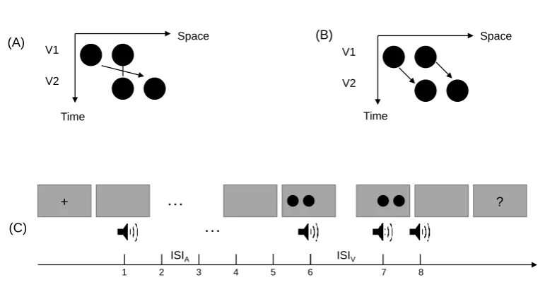
Figure 1.Ternus display and stimulus configurations. Two alternative motion percepts of the

Ternus display: (A): ‘element’ motion for short ISIs, with the middle dot perceived as

remaining static while the outer dots are perceived to move from one side to the other. (B)

‘group’ motion for long ISIs, with the two dots perceived as moving in tandem. (C) Schematic

illustration of the stimulus configurations used in the experiments. The auditory sequence

consisted of 8 to 10 beeps. Two of the beeps (the 6th and the 7th_{) were synchronously paired}

with two visual Ternus frames which were separated by a visual ISI (ISIV(isual)) that varied

from 50 to 230 ms (for the critical beeps, ISIV(isual) = ISIA(ditory)). The other auditory ISIs

(ISIA(ditory)) were systematically manipulated such that the mean of the ISIA preceding the

visual Ternus display was 50–70 ms shorter than, equal to, or 50–70 ms longer than the

transition threshold between the element- and group-motion percepts of the visual Ternus

events. The transition threshold was first estimated individually for each observer in a

pre-test session. During the experiment, observers were simply asked to indicate the type of

visual motion (‘element’ or ‘group’) that they had perceived, while ignoring the beeps.

Mono sound beeps (1000 Hz, 65 dB, 30 ms) were generated and delivered via an

M-Audio card (Delta 1010) to a headset (Philips, SHM1900). To ensure accurate timing of

the auditory and visual stimuli, the duration of the visual stimuli and the synchronization of

the auditory and visual stimuli were controlled via the monitor’s vertical synchronization

V1

V2

Space

Time

Space

Time V1

V2

(A) (B)

(C)

+ … ?

…

1 2 3 4 5 6 7 8

9

pulses. The experimental program was written with Matlab (Mathworks Inc.) and the

Psychophysics Toolbox (Brainard, 1997).

Experimental Design

Practice

Prior to the formal experiment, participants were familiarized with visual Ternus

displays of either typical element motion (with an ISIV of 50 ms) or typical group motion

(ISIV of 260 ms) in a practice block. They were asked to discriminate the two types of

apparent motion by pressing the left or the right mouse button, respectively. The mapping

between response button and type of motion was counterbalanced across participants. During

practice, when a response was made that was inconsistent with the typical motion percept,

immediate feedback appeared on the screen showing the typical response (i.e., element or

group motion). The practice session continued until the participant reached a conformity of

95%. All participants achieved this criterion within 120 trials, given that the two extreme ISIs

used (50 and 260 ms, respectively) gave rise to non-ambiguous percepts of either element

motion or group motion.

Pre-test

For each participant, the transition threshold between element and group motion was

determined in a pre-test session. A trial began with the presentation of a central fixation cross

for 300 to 500 ms. After a blank screen of 600 ms, the two Ternus frames were presented

synchronized with two auditory tones (i.e., baseline: ISIV = ISIA); this was followed by a

blank screen of 300 to 500 ms, prior to a screen with a question mark prompting the

participant to make a two-forced-choice response indicating the type of perceived motion

(element or group motion). The ISIV between the two visual frames was randomly selected

from one of the following seven intervals: 50, 80, 110, 140, 170, 200, and 230 ms. There were

40 trials for each level of ISIV, counterbalanced with left- and rightward apparent motion. The

presentation order of the trials was randomized for each participant. Participants performed a

total of 280 trials, divided into 4 blocks of 70 trials each. After completing the pre-test, the

psychometric curve was fitted to the proportions of group motion responses across the seven

intervals (see Data Analysis and Modeling). The transition threshold, that is, the point of

10

percepts, was calculated by estimating the ISI at the point on the fitted curve that

corresponded to 50% of group motion reports. The just noticeable difference (JND), an

indicator of the sensitivity of apparent motion discrimination, was calculated as half of the

difference between the lower (25%) and upper (75%) bounds of the thresholds from the

psychometric curve.

Main Experiments

In the main experiments, the procedure of visual stimulus presentation was the same as

in the pre-test session, except that prior to the occurrence of the two Ternus display frames, an

auditory sequence consisting a variable number of 6–8 beeps was presented (see below for the

details of the onset of the Ternus display frames relative to that of the auditory sequence). As

in the pre-test, the onset of the two visual Ternus frames (each presented for 30 ms) was

accompanied by a (30-ms) auditory beep (i.e., ISIV = ISIA). A trial began with the

presentation of a central fixation marker, randomly for 300 to 500 ms. After a 600-ms blank

interval, the auditory train and the visual Ternus frames were presented (see Figure 1c),

followed sequentially by a blank screen of 300 to 500 ms and a screen with a question mark at

the screen center prompting participants to indicate the type of motion they had perceived:

element versus group motion (non-speeded response). Participants were instructed to focus on

the visual task, ignoring the sounds. After the response, the next trial started following a

random inter-trial interval of 500 to 700 ms.

In Experiment 1 (regular sound sequence), the audiovisual Ternus frames was preceded

by an auditory sequence of 6–8 beeps with a constant inter-stimulus interval (ISIA),

manipulated to be 70 ms shorter than, equal to, or 70 ms longer than the transition threshold

estimated in the pre-test. The total auditory sequence consisted of 8–10 beeps, including those

accompanying the two visual Ternus frames, with the latter being inserted mainly at the 6th–

7th positions, and followed by 0–2 beeps (number selected at random), to minimize

expectations as to the onset of the visual Ternus frames. Visual Ternus frames were presented

on 75% of all trials (504 trials in total). The remaining 25% were catch trials (168 trials) to

break up anticipatory processes. All trials were randomized and organized in 12 blocks, each

of 56 trials. The ISIV between the two visual Ternus frames was randomly selected from one

11

In Experiment 2 (irregular sound sequence), the settings were the same as in

Experiment 1, except that the auditory trains were irregular: the ISIA between adjacent beeps

in the auditory train (except the ISIA between the beeps accompanying the visual Ternus

frames) were varied ±20 ms uniformly and randomly around (i.e., they were either 20 ms

shorter or 20 ms longer than) a given mean interval (three levels: 70 ms shorter than, equal to,

or 70 ms longer than the individual transition threshold).

Experiment 3 introduced two levels of variability in the auditory-interval sequences

with 8–10 beeps: a low coefficient of variance (CV, the standard deviation divided by the

mean) of 0.1 and, respectively, a high CV of 0.3. For each CV condition, three arithmetic

mean intervals were used: 50 ms shorter than, equal to, or 50 ms longer than the estimated

transition threshold. The intervals were randomly generated from a normal distribution with a

given mean and CV. The number of the experimental trials was 1008, and the catch trials

totaled 336. All trials were randomized and organized in 24 blocks, each block containing 56

trials.

Experiment 4 used three types of auditory sequences, each consisting of 6 intervals: (i)

Baseline auditory sequence: three intervals, of 110, 140, and 170 ms, were repeated twice in

random order; in this baseline condition, the arithmetic mean (AM = 140 ms) was near-equal

to the geometric mean (GM = 138 ms). (ii) AM-deviated sequence: 6 intervals were

constructed from ISIA of 70, 140, and 280 ms, which were arranged randomly (AM = 163 ms

> GM = 140 ms); (iii) GM-deviated sequence: 6 intervals constructed from ISIA 50, 140, and

230 ms, arranged randomly (GM = 117 ms < AM = 140 ms). The audiovisual Ternus frames

were appended at the end of these sequences. The number of experimental trials was 504

(there were no catch trials), which were presented randomized and organized in 12 blocks,

each of 42 trials.

To exclude potential confounding by a recency effect, in Experiment 5, we compared

two auditory sequences: one with a geometric mean 70 ms shorter than the transition

threshold of visual Ternus motion (henceforth referred to as ‘Short’ condition), and the other

with a geometric mean 70 ms longer than the transition threshold (‘Long’ condition). Instead

of completely randomizing the five auditory intervals (excepting the final synchronous

12

the Ternus display was fixed at the transition threshold for both sequences. The remaining

four intervals were chosen randomly such that the CV of the auditory sequence was in the

range between 0.1 and 0.2. This manipulation was expected to minimize the influence of any

potential recency effect engendered by the last auditory interval. The audiovisual Ternus

frames were appended at the end of these sequences on trials (i.e., 672 out of a total of 784

trials) on which the Ternus display appeared at the end of the sound sequence (the ‘onset’ of

the first visual frame was synchronized with 6th beep). The remaining (112) trials were catch

trials, with 56 trials each on which the Ternus displays occurred at the beginning of the sound

sequence (i.e., the onset of the first visual frame was synchronized with the second beep) or,

respectively, at middle temporal locations (i.e., the onset of the first visual frame was

synchronized with the 4th beep). These catch trials were introduced to prevent participants

from consistently anticipating the visual events to occur at the end of the sound sequence. The

total 784 trials were randomized and organized in 14 blocks, each of 56 trials.

Data analysis and Modeling

We used the R package Quickpsy (Linares & López-Moliner, 2016) to fit psychometric

curves with upper and lower asymptotes, which provide better estimates of the thresholds

(Wichmann & Hill, 2001). Bayesian modeling was also conducted with R. We first calculated

the response proportions for the baseline tests with (audio-) visual Ternus apparent motion

and for the formal experiments, as well as fitting the corresponding cumulative Gaussian

psychometric functions. Based on the psychometric functions, we could then estimate the

discrimination variability of Ternus apparent motion (i.e., 𝜎𝑚) based on the standard

deviation of the cumulative Gaussian function. The parameters of the Bayesian models (see

Bayesian modeling section below) were estimated by minimizing the prediction errors using

the R optim function. Our raw data together with the source code of statistical analyses and

Bayesian modeling are available at the github repository:

https://github.com/msenselab/temporal_averaging.

13

Experiments 1 and 2: Both regular and irregular auditory intervals alter the visual

motion percept.

We manipulated the intervals between successive beeps (i.e., the ISIA prior to the Ternus

display) to be either regular or irregular, but with their arithmetic mean being either 70 ms

shorter, equal to, or 70 ms longer than the transition threshold (measured in the pre-test)

between element- and group-motion reports (for both regular and irregular ISIA). Auditory

sequences with a relatively long mean auditory interval, as compared to a short interval, were

found to elicit more reports of group motion, as indicated by the smaller PSEs (Figure 2), for

both regular intervals, F(2,40)=12.22, p<0.001, 𝜂𝑔2 = 0.112, and irregular intervals,

F(2,42)=8.25, p<0.001, 𝜂𝑔2=0.04. That is, the perceived visual interval (which determines the

ensuing motion percept) was assimilated by the average of the preceding auditory intervals,

regardless of whether the auditory intervals were regular or irregular. Post-hoc Bonferroni

comparison tests revealed that this assimilation effect was mainly driven by the short auditory

intervals in both experiments: ps were 0.001, 0.00001, and 0.57 for the comparisons -70 vs. 0

ms, -70 vs. 70 ms, and, respectively, 0 vs. 70 ms for the regular intervals; and 0.015, 0.0002,

0.77 for the comparisons of the irregular intervals (Figure 2C and 2D).

0.00 0.25 0.50 0.75 1.00

50 100 150 200

ISI (ms) P ro p . o f g ro u p m o ti o n −70 0 70 A 0.00 0.25 0.50 0.75 1.00

50 100 150 200

ISI (ms) P ro p . o f g ro u p m o ti o n −70 0 70 B * * 100 120 140 160

−70 0 70

Relative mean auditory interval (ms)

P S E s ( m s ) C * * 100 120 140 160

−70 0 70

Relative mean auditor y interval (ms)

14

Figure 2. The average means of both regular and irregular auditory sequences influence

the visual motion percept. (A) Regular auditory-sequence condition: For a typical

participant, mean proportions of group-motion responses as a function of the probe visual

interval (ISIv), and fitted psychometric curves, for auditory sequences with different

(arithmetic) mean intervals relative to the individual transition thresholds; the

relative-interval labels (-70, 0, and 70) denote the three conditions of the mean auditory

interval being 70 ms shorter than, equal to, and 70 ms longer than the pre-test transition

threshold, respectively. (B) Irregular auditory-sequence condition: for a typical participant,

mean proportions of group-motion responses and fitted psychometric curves. (C) Mean PSEs

as a function of the relative auditory interval for the regular-sequence condition; error bars

represent standard errors of the means. (D) Mean PSEs as a function of the relative auditory

interval for the irregular-sequence condition; error bars represent standard errors of the

means.

The fact that a crossmodal assimilation effect was obtained even with irregular auditory

sequences suggests that the effect is unlikely due to temporal expectation, or a general effect

of auditory entrainment (Jones, Moynihan, MacKenzie, & Puente, 2002; Large & Jones,

1999). In addition, the assimilation effect observed is unlikely due to a recency effect. To

examine for such an effect, we split the trials into two categories according to the auditory

interval that just preceded the visual Ternus interval: short and long preceding intervals with

reference to the auditory mean interval. The length of the immediately preceding interval

failed to produce any significant modulation of apparent visual motion, F(1, 22) = 2.14, p =

0.15. An account in terms of a recency effect was further ruled out by a dedicated control

experiment that directly fixed the last auditory interval (see Experiment 5 below).

Furthermore, in the regular condition, the mean JNDs (±SE) for the three ISIV conditions

[34.9 (±3.1), 30.5 (±3.4), and 28.4 (±2.9) ms for the ISIV 70 ms shorter, equal to, and,

respectively, 70 ms longer relative to the transition threshold] were larger than the JND for

the threshold (baseline) condition (18.8 (±1.2) ms; p=0.001, p=0.002, and p=0.033 for the

shorter, equal, and longer conditions vs. the 'threshold'), without differing amongst

15

p=0.001, 30.6 (±2.3), p=0.005, and 27.2 (±2.2) ms compared to the baseline 18.6 (±2.1) ms,

without differing amongst themselves (all ps>0.1). The worsened sensitivities in the three

conditions with auditory beep trains suggest that the assimilation effect observed here was not

attributable to attentional entrainment, as attentional entrainment would have been expected

to enhance the sensitivity.

Experiment 3: Variability of auditory intervals influences visual Ternus apparent

motion.

According to quantitative models of multisensory integration (Ernst & Di Luca, 2011;

Shi, Church, & Meck, 2013), the strength of the assimilation effect would be determined by

the variability of both the auditory intervals and the visual Ternus interval, assuming that

information is integrated from all intervals. According to optimal full integration, high

variance of the auditory sequence would result in a low auditory weight in audiovisual

integration, leading to a weaker assimilation effect compared to low variance. To examine for

effects of the variance of the auditory intervals on visual Ternus apparent motion, we directly

manipulated the relative standard deviation of the auditory intervals while fixing their

arithmetic mean. One key property of time perception is that it is scalar (Church, Meck, &

Gibbon, 1994; Gibbon, 1977), that is, the estimation error increases linearly as the time

interval increases, approximately following Weber’s law. Given this, we used coefficients of

variance (CVs), that is, the ratio of the standard deviation to the mean, to manipulate

standardized variability across multiple auditory intervals. Specifically, we compared a low

CV (0.1) with a high CV (0.3) condition, with an orthogonal variation of the (arithmetic)

mean auditory interval: 50 ms shorter, equal to, or 50 ms longer than the pre-determined

transition threshold.

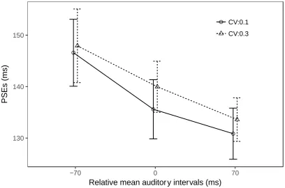
The main effect of mean interval was significant, F(2,30)=11.8, p<0.001, 𝜂𝑔2 =

0.078, with long intervals leading to more reports of group motion (i.e., lower PSEs: mean

PSE of 132±4.6 ms), short intervals to fewer reports of group motion (i.e., higher PSEs: mean

PSE of 147±6.7 ms), and equal intervals to an intermediate proportion of group-motion

reports (mean PSE of 138±5.3 ms). Post-hoc Bonferroni comparisons revealed this pattern to

16

and equal intervals (p<0.01) and the short and long intervals (p<0.001), but not between the

equal and long intervals (p = 0.49). Interestingly, the main effect of CV was significant

(though the effect size is small), F(1,15) = 5.29, p<0.05, 𝜂𝑔2 = 0.044, while the interaction

between mean interval and CV was not, F(2, 30)=0.31, p=0.73, 𝜂𝑔2 = 0.0008 (Figure 3).

Further examination for a (potentially confounding) recency effect, adopting the same

comparison as for the previous experiments, yielded no evidence that the main effects we

obtained are attributable to the length of the auditory interval immediately preceding the

visual interval, F(1,15) = 0.33, p = 0.55.

Figure 3. PSEs between element- and group-motion reports for auditory beep trains with a

low and a high coefficient of (auditory-interval) variance (CV, 0.1 or 0.3), as a function of the

(arithmetic) mean auditory interval (50 ms shorter, equal to, or 50 ms longer than the pre-test

transition threshold).

These results are interesting in two respects. First, according to mandatory, full Bayesian

integration (see Modeling section below for details), auditory-interval variability should affect

the weights of the crossmodal temporal integration (Buus, 1999; Shi et al., 2013), with greater

variance lessening the influence of the average auditory interval. Accordingly, the slopes of

130 140 150

−70 0 70

Relative mean auditor y intervals (ms)

P

S

E

s

(

m

s

)

CV:0.1

17

the fitted lines in Figure 2 would be expected to be flatter under the high compared to the low

CV condition, yielding an interaction between mean interval and CV. The fact that this

interaction was non-significant suggests that the ensemble mean of the auditory intervals is

not fully integrated with the visual interval (we will return to this point in the next, Modeling

section). Second, the downward shift of the PSEs in the low, compared to the high, CV

condition indicates that the perceived auditory mean interval (that influences the audio-visual

integration) is actually not the arithmetic mean (‘AM’) that we manipulated. An alternative

account of this shift may derive from the fact the auditory sequences with higher CV have a

lower geometric mean (‘GM’) than the sequences with low variance, that is: the perceived

ensemble mean is likely geometrically encoded. Experiment 4 was designed to address this

(potential) confound by directly comparing the effects of ensemble coding based on the

geometric versus the arithmetic mean.

Experiment 4: Perceptual averaging of auditory intervals assimilates the visual interval

towards the geometric, rather than the arithmetic, mean.

In Experiment 4, we compared three types of auditory sequence in our audiovisual

Ternus apparent motion paradigm: a baseline sequence, an AM-deviated sequence, and a

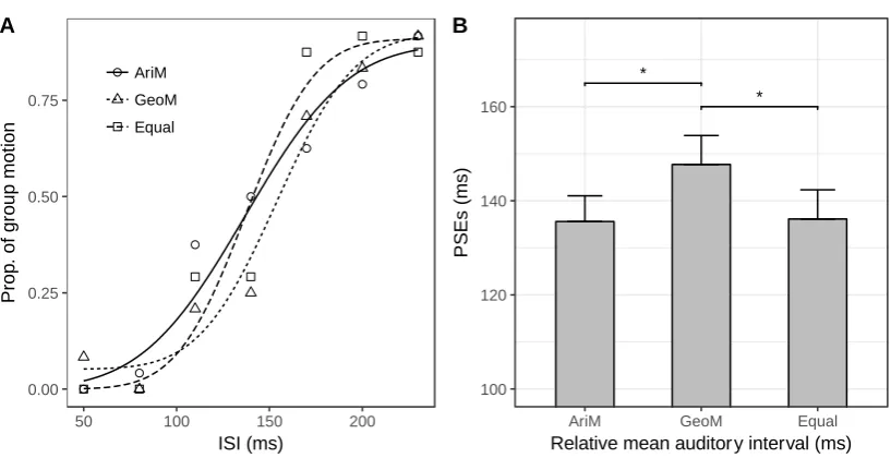
GM-deviated sequence.The PSEs were 136 (±5.46), 148 (±6.17), and 136 (±6.2) ms for the

AM-deviated (AriM), the GM-deviated (GeoM), and the baseline conditions, respectively,

F(2, 22)=8.81, p<0.05, ηg2 = 0.08 (Figure 4). Bonferroni-corrected comparisons revealed the

transition threshold to be significantly larger for the GeoM compared to the baseline

condition, p<0.01, whereas there was no difference between the AriM and the baseline

condition, p=1. This pattern indicates that ensemble coding of the auditory interval

18

Figure 4. Auditory geometric mean assimilates visual Ternus apparent motion. (A) For a

typical participant, mean proportions of group-motion responses as a function of the probe

visual interval (ISIv), and fitted psychometric curves, for the three auditory-sequence

conditions: (i) sequence of intervals with larger arithmetic mean (AriM); (ii) sequence of

intervals with smaller geometric mean (GeoM); (iii) baseline sequence with equal arithmetic

and geometric means (140 ms). (B) Mean PSEs (with error bars representing standard errors

of the means) for the three auditory-sequence conditions. Compared to the baseline sequence,

the GeoM sequence (with the smaller geometric mean) produced a significant shift of the

visual transition threshold, whereas the AriM sequence (with the larger arithmetic mean) did

not.

Experiment 5: Auditory sequences with the last interval fixed

In Experiments 1–3, we split the data according to the last interval (i.e., the interval

preceding the visual Ternus display) of the auditory sequence into two categories (short vs.

long), which failed to reveal any influence of the last interval. In Experiment 5, we formally

manipulated the last interval by fixing it at the respective transition threshold for the ‘Short’

and ‘Long’ auditory sequences (i.e., sequences with the smaller and, respectively, larger

geometric means). Figure 5 depicts the responses of a typical participant from Experiment 5.

The PSEs were 153.1 (±7.3) and, respectively, 137.9 (±9.1) for the ‘Short and ‘Long’

conditions, respectively, t(11)=3.640, p<0.01. That is, reports of element motion were more 0.00

0.25 0.50 0.75

50 100 150 200

ISI (ms) P ro p . o f g ro u p m o ti o n AriM GeoM Equal A * * 100 120 140 160

AriM GeoM Equal Relative mean auditor y interval (ms)

19

dominant in the ‘Short’ than in the ‘Long’ condition, replicating the findings of the previous

experiments. In other words, it was the mean auditory interval, rather than the last interval

(prior to the Ternus frames), that assimilated visual Ternus apparent motion. Given this, the

audiovisual interactions we found here are unlikely attributable to a recency effect.

Figure 5. Mean proportions of group-motion responses from a typical participant as a

function of the probe visual interval (ISIv), and fitted psychometric curves, for the two

geometric mean conditions: the ‘Short’ sequence (with the smaller geometric mean) and the

‘Long’ sequence (with the larger geometric mean).

Bayesian modeling

To account for the above findings, we implemented, and compared two variants of

Bayesian integration models: mandatory full Bayesian integration and partial Bayesian

integration. If the ensemble-coded auditory-interval mean (𝐴) and the audiovisual Ternus

display interval (𝑀) are fully integrated according to the maximum likelihood estimation

(MLE) principle (Ernst & Banks, 2002), and both are normally distributed (e.g., fluctuating

due to internal Gaussian noise) – that is: 𝐴 ∼ 𝑁(𝐼𝑎, 𝜎𝑎), 𝑀 ∼ 𝑁(𝐼𝑚, 𝜎𝑚) – the expected

optimally integrated audio-visual interval, which yields minimum variability, can be predicted

as follows:

𝐼^𝑓𝑢𝑙𝑙 = 𝑤𝐼𝑎+ (1 − 𝑤)𝐼𝑚, (1)

where 𝑤 =_𝜎1 𝑎2/(

1 𝜎𝑎2+

1

𝜎𝑚2) is the weight of the averaged auditory interval, which is

proportional to its reliability. Note that full optimal integration is typically observed when the 0.00

0.25 0.50 0.75 1.00

50 100 150 200

20

two ‘cues’ are close to each other, but it breaks down when their discrepancy becomes too

large (Kording et al., 2007; Parise, Spence, & Ernst, 2012; Roach et al., 2006). In our study,

the Ternus interval and the mean auditory interval could differ substantially on some trials

(e.g., visual interval of 50 ms paired with mean auditory interval of 210 ms). Given this, a

more appropriate model would need to take a ‘discrepancy’ prior and the causal structure

(Kording et al., 2007) of audio-visual temporal integration into consideration. Thus, similar to

(Roach et al., 2006), here we assume that the probability of full integration 𝑃𝑎𝑚 depends on

the discrepancy between the mean auditory and Ternus intervals:

𝑃_𝑎𝑚∼ 𝑒−(𝐼𝑎−𝐼𝑚)2/𝜎𝑎𝑚2 , ₍₂₎

where 𝜎𝑎𝑚2 is the variance of the sensory measures of the discrepancy between the ensemble

mean of the auditory intervals and the visual interval. 𝑃𝑎𝑚 will vary from trial to trial,

depending on the discrepancy between the mean auditory interval and the visual interval.

Thus, a more general, partial integration model would predict:

𝐼^_𝑎𝑣 = 𝑃_𝑎𝑚𝐼^_{𝑓𝑢𝑙𝑙}+ (1 − 𝑃_𝑎𝑚)𝐼_𝑣. (3)

Combined with equation (1), equation (3) can be simplified as follows:

𝐼^_𝑎𝑣 = (1 − 𝑤𝑃_𝑎𝑚)𝐼_𝑣+ 𝑤𝑃_𝑎𝑚𝐼_𝑎. (4)

To compare the full-integration and partial-integration models, we took into account the

data from those of our experiments that manipulated the auditory-interval regularity and

variability (Experiments 1–3; we excluded Experiments 4 and 5, as these did not include a

baseline task of Ternus apparent-motion perception; see Methods section). Given that the

baseline task provided an estimate of 𝜎𝑚, there is one parameter – 𝜎𝑎 – for the

full-integration model and two parameters – 𝜎𝑎 and 𝜎𝑎𝑚 – for the partial-integration model,

which require parameter fitting. This was carried out using the optimization algorithm

L-BFGS in R (see our source code at https://github.com/msenselab/temporal_averaging). We

assessed the goodness of the resulting fits by means of coefficients of determination (𝑅2) and

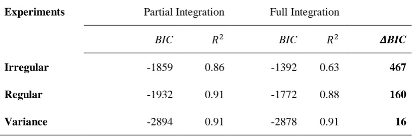
Bayesian information criteria (BIC). The BIC and 𝑅2 scores are presented in Table 1. As can

21

experiments, clearly favoring the partial-integration model (Kass & Raftery, 1995). The 𝑅2

values also confirms this.

Table 1. Model comparison using BIC and 𝑹𝟐 for the partial- and full-integration model

Experiments Partial Integration Full Integration

BIC 𝑅2 BIC 𝑅2 𝜟BIC

Irregular -1859 0.86 -1392 0.63 467

Regular -1932 0.91 -1772 0.88 160

Variance -2894 0.91 -2878 0.91 16

Note. The differential BICs scores revealed the partial-integration model to outperform

the full-integration model across all experiments (very strong evidence in all

experiments: 𝜟BIC >10).

To visualize how well the partial-integration model predicts behavioral performance, we

calculated the predicted mean responses based on the partial-integration model for individual

visual ISIs across all experimental conditions. Figure 6 illustrates the predictions, indicated by

curves, together with the observed mean responses, indicated by shape points. As can be seen,

the predicted mean responses are within one standard error of the observed mean responses

22

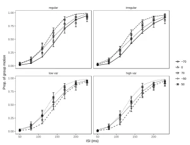
Figure 6. Mean behavioral responses (proportion of group-motion reports, indicated by

shape points) and responses predicted by the partial-integration model (indicated by curves)

as a function of the ISIV of the Ternus display, separately for auditory sequences with

different (arithmetic) mean intervals relative to the individual transition thresholds. The

relative-interval labels (-70, -50, 0, 50, and 70 [ms]) denote the magnitude of the difference

between the mean auditory interval and the transition threshold. Error bars denote standard

errors of means (±SEM).

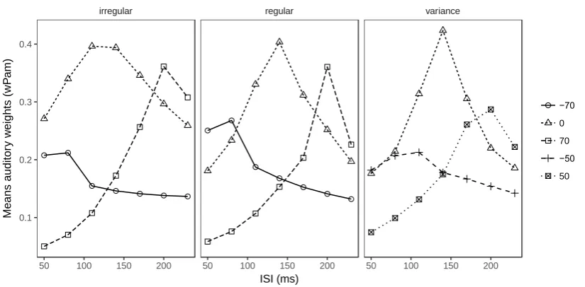
The key difference between the full- and partial-integration models is that the latter takes

the probability of crossmodal integration into account; accordingly, the weight of the auditory

ensemble intervals (i.e., 𝑤𝑃𝑎𝑚) depends on the difference between the ensemble mean of the

auditory intervals and the visual interval. This can be seen in Figure 7, which illustrates the

dynamic changes of the auditory weights across the various audio-visual interval discrepancy

conditions. All three experiments exhibit a similar pattern: weights are at their peak when the

visual interval and the auditory mean intervals are close to each other. For example, the peaks

for the relative intervals of 0 ms (i.e., the auditory mean intervals were set to the individual

visual thresholds) are around 140 ms, close to the mean visual transition threshold (134.6 ms

low var high var

regular irregular

50 100 150 200 50 100 150 200

23

for regular and 135.3 ms for irregular sequences, and 139.0 ms for low and 144.8 ms for high

variance). For relative intervals of 70 ms, the peaks are shifted rightwards; and for relative

intervals of -70 ms, they are shifted leftwards.

Figure 7. Predicted weights (i.e., 𝑤𝑃𝑎𝑚, based on the partial-integration model) of the

auditory ensemble intervals as a function of the ISIV of the Ternus display, separately for

auditory sequences with different (arithmetic) mean intervals relative to the individual

transition thresholds. The relative-interval labels (-70, -50, 0, 50, and 70 ms) denote the

magnitude of the difference between the mean auditory interval and the transition threshold.

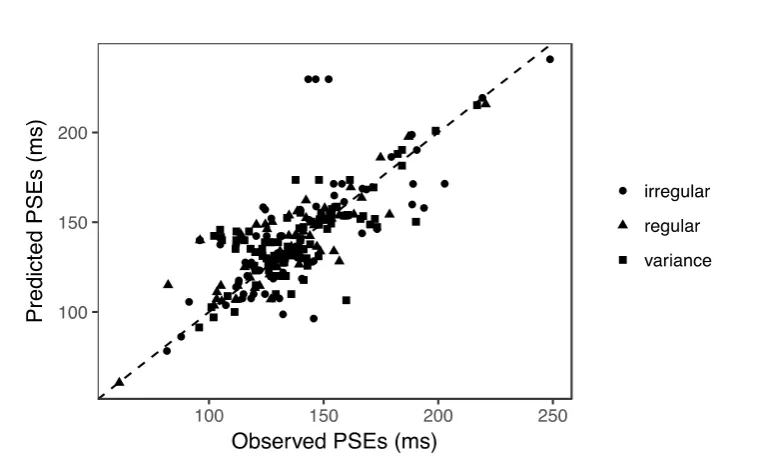
Based on the responses predicted by the partial-integration model, we further calculated

the predicted PSEs. Figure 8 shows a linear relation between the observed and predicted PSEs

for all experiments. Linear regression revealed a significant linear correlation, with a slope of

0.978 and an adjusted 𝑅2 = 0.983. The full-integration model, by contrast, produced flat

psychometric curves for 6% of the individual conditions in Experiments 1 and 2 (due to the

weight of the mean auditory interval approaching 1), which yielded unreliable estimates of

the corresponding PSEs. This led to lower predictive power compared to the

partial-integration model, as evidenced by the BIC and R2 _{scores (Table 1). Thus, taken}

together, the partial-integration model can well explain the behavioral data that we observed.

irregular regular variance

50 100 150 200 50 100 150 200 50 100 150 200

24

Figure 8. Predicted PSEs versus observed PSEs for all experiments. Each dot represents the

PSE of one particular observer in a given experimental condition. Shape points represent the

four auditory-sequence manipulations. Linear regression revealed a significant high

correlation (𝑅2= 0.983) and a slope of 1.008.

General Discussion

Using an audiovisual Ternus apparent motion paradigm, we conducted five experiments

on audiovisual temporal integration with regular and irregular auditory sequences presented

prior to the (audio-) visual Ternus display. We found that perceptual averaging of both regular

(Experiment 1) and irregular auditory sequences (Experiments 2 and 3) greatly influenced the

timing of the subsequent visual interval, as expressed in systematic changes of the transition

threshold in visual Ternus apparent motion: longer mean auditory intervals elicited more

reports of group motion, whereas shorter mean intervals gave rise to dominant element

motion. In Experiment 4, we further found that the geometric mean of the auditory intervals

can explain the audiovisual interaction better than the arithmetic mean. Further (post-hoc)

analyses and a purpose-designed experiment (Experiment 5) effectively ruled out an

explanation of these findings in terms of a recency effect, that is, a dominant influence of the

last interval prior to the Ternus frames. Using a Bayesian integration approach, we showed

that the behavioral responses are best predicted by partial-cue integration, rather than by full

25

a train of beeps that forms the background context of the visual task to play a critical role in

crossmodal temporal integration, even when participants are asked to ignore the auditory

stimuli.

Perceptual averaging and crossmodal temporal rate interaction

Extracting key statistical information from sets of objects or events in our environment

would provide us with a perceptual strategy to cope with limitations in attentional and

working memory capacity (Allik, Toom, Raidvee, Averin, & Kreegipuu, 2014; Chetverikov,

Campana, & Kristjansson, 2016) – given that we can have conscious access to only very few

items from the total amount of information received by our senses at any one time (e.g.,

Bundesen, Habekost, & Kyllingsbaek, 2005; Cohen, Dennett, & Kanwisher, 2016; Cowan,

2001; Marois & Ivanoff, 2005). In this situation, perceptual averaging would endow us with

an efficient and, in evolutionary terms, competitive solution to overcome bandwidth

limitations (McClelland & Bayne, 2016), thus constituting one of the underlying

computational principles for selecting appropriate actions to achieve our current behavioral

goals.Clearly, timing is fundamental for dynamic perception, and therefore unlikely to be an

exception with regard to perceptual averaging (Hardy & Buonomano, 2016; McDermott &

Simoncelli, 2011). For instance, when listening to a piece of music, we can immediately tell

the average tempo, even though the individual ‘notes’ may not be well remembered. And

when watching a field of runners in a competition, we immediately know whether it is a slow

or a fast race overall.

Research on the audiovisual interaction in (crossmodal) event timing has shown auditory

rate to have a pronounced influence on visual rate perception (Recanzone, 2003, 2009; Roach

et al., 2006; Shipley, 1964). The visual temporal rate is often assimilated to the auditory rate,

owing to the higher temporal resolution of audition compared to vision. Of note, however, the

extant studies have used only regular temporal sequences, thus leaving it an open question

whether the mechanism underlying the assimilation effect is perceptual averaging, temporal

entrainment, or a recency effect from the latest auditory interval. On this background, the

present study examined how irregular auditory sequences influence visual interval timing –

26

is the temporal averaging of the auditory sequence (regardless of its regularity) that exerted a

great influence on the visual interval.

Temporal averaging and geometric encoding

The present results indicate that the geometric mean well encapsulates the summary

statistics of the temporal structure hidden in a complex multisensory stream (Hanson, Heron,

& Whitaker, 2008; Heron, Roach, Hanson, McGraw, & Whitaker, 2012). Previous work on

numerosity had already suggested that the mental scales underlying the representation of

visual numerosity and temporal magnitudes are best characterized as being non-linear, as

opposed to linear, in nature (Dehaene, 2003; Dehaene et al., 2008; Nieder & Miller, 2003,

2004; Rips, 2013). For example, adults from the Mundurucu, an Amazonian indigenous tribe

with a limited number lexicon, map numerical quantities onto space in a logarithmic fashion

( Dehaene et al., 2008; but see Cicchini, Arrighi, Cecchetti, Giusti, & Burr, 2012). A seminal

study by Allan and Gibbon also showed that temporal bisection coincided with the geometric

mean of the two reference durations (Allan & Gibbon, 1991). Our findings reveal that

extraction of the geometric mean also underlies temporal averaging – and this might well be a

principle shared by a broad range of mechanisms coding ‘magnitude’ in perception (Walsh,

2003).

Partial integration in crossmodal temporal processing

Research on multisensory integration has shown that the ‘proximity’ and ‘similarity’ of

the spatiotemporal structure of multisensory signals – technically, their cross-correlation in

time (and space) – is critical for inferring an underlying common source to both signal

streams (Parise & Ernst, 2016; Parise et al., 2012). Accordingly, highly correlated audiovisual

events are likely perceived as arising from a single, multisensory source. Roach and

colleagues (2006) quantified this for audiovisual rate perception by introducing a disparity

prior, that is, their model assumes that the strength of crossmodal temporal integration is

dependent on the disparity between the auditory and visual temporal rates.

In the present study, by comparing two variants of Bayesian integration models, full and

27

averaging of the preceding, task-irrelevant auditory intervals assimilates the subsequent,

perceived visual interval between the Ternus display frames. The modeling results indicate

that the ensemble mean of the auditory intervals only partially integrates with the visual

interval, dependent on the time disparity between the two: when the mean of the auditory

intervals is close to the visual interval, they are optimally integrated according to the MLE

principle; in contrast, if the ensemble mean deviates grossly from the visual interval, partial

integration, based on the crossmodal disparity, provides a superior account of the behavioral

data to mandatory, full integration. However, in contrast to full integration, partial integration

requires participants to take both the mean statistics and the crossmodal disparity into

account. This is consistent with a large body of literature on temporal contextual modulation,

within the broader framework of Bayesian optimization (Jazayeri & Shadlen, 2010; Roach,

McGraw, Whitaker, & Heron, 2017; Shi et al., 2013), where prior information (e.g., history

information or a discrepancy prior) is incorporated in multisensory integration.

Perceptual averaging and temporal entrainment

One important question to be considered is whether the assimilation effect induced by

perceptual averaging can be distinguished, at root, from attentional entrainment. In the typical

auditory entrainment paradigm, the rhythm itself is irrelevant with respect to the visual target

events that are to be detected (or discriminated), though temporal expectations induced by the

rhythm influence attentional selection of the target (Lakatos, Karmos, Mehta, Ulbert, &

Schroeder, 2008). Rhythmically (i.e., with temporal attention) anticipated target events are

detected or discriminated more rapidly than early or late events that are out of phase with the

peaks of the attentional modulation induced by the entrainment (Ronconi & Melcher, 2017).

Irregular rhythms, by contrast, have been shown to disrupt temporal attention, as evidenced

by reduced benefits for responding to the target events (Miller, Carlson, & McAuley, 2013).

Importantly, in present study, both regular and irregular auditory sequences did reduce (rather

than enhance) the sensitivity of discriminating Ternus apparent (i.e., element vs. group)

motion, as evidenced by the increased JNDs. In contrast, the averaged temporal intervals,

whether these formed a regular or irregular series, were automatically integrated with the

28

motion percepts. This ‘dissociation’ implies that the assimilation effects demonstrated here

reflect a genuine, automatic perceptual averaging mechanism that operates independently of

attentional entrainment processes.

Irrelevant context in multisensory perceptual averaging

One might ask why the brain would at all take into account entirely task-irrelevant

contexts – such as, in the present study, the (mean of the) intervals of an irrelevant auditory

sequence – in multisensory integration. As revealed by our experiments, the discrimination

sensitivity for visual apparent motion became actually worse and the motion percept became

biased by including the irrelevant auditory sequence. Note however that, in the real world,

there are normally strong associations and correlations in the multisensory inputs – so that

drawing on this additional information often increases the reliability of perceptual estimates.

For example, the rhythmic sound pattern produced by a train moving along the track would

help us improve our estimation of the train’s speed, given that the tempo of the track sound is

linearly correlated with the speed of the train. Indeed, convergent evidence suggests that

multisensory integration can reduce the uncertainty of the final estimates in many situations

(Ernst & Banks, 2002; Ernst & Di Luca, 2011). However, integrating multiple sources of

information that deviates from the currently relevant information may engender unwanted

biases. Such contextual modulations have been reported in various forms. For example, when

performing a series of time estimations, observers’ judgment of a given interval is biased

toward the intervals that they just experienced (Jazayeri & Shadlen, 2010) – which is known

as a central-tendency effect (Petzschner, Glasauer, & Stephan, 2015; Shi & Burr, 2016; Shi et

al., 2013). A similar contextual modulation is also at work in the so-called time-shrinking

illusion, in which the percept of the last auditory interval is assimilated by the preceding

intervals (Nakajima, ten Hoopen, Hilkhuysen, & Sasaki, 1992; Nakajima et al., 2004), as well

as in audiovisual interval judgments when auditory and visual intervals are presented

sequentially (Burr et al., 2013). The present study demonstrated that such an audiovisual

integration still occurs even when participants are explicitly told to ignore the (task-irrelevant)

auditory sequence, suggesting that processes of top-down control cannot fully shield visual

29

Conclusion

It has long been known that auditory flutter drives visual flicker (Shipley, 1964) – a

typical phenomenon of audiovisual temporal interaction with regular auditory sequences.

Here, in five experiments, we demonstrated that irregular auditory sequences also capture

temporal processing of subsequently presented visual (target) events, measured in terms of the

biasing of Ternus apparent motion. Importantly, it is the geometric averaging of the auditory

intervals that assimilates the visual interval between the two visual Ternus display frames,

thereby influencing decisions on perceived visual motion. Further work is required to

examine whether the principles of geometric averaging and partial crossmodal integration

demonstrated here (for an audiovisual dynamic perception scenario) generalize to other

perceptual mechanisms underlying magnitude estimation in multisensory integration.

Context of the Research

Perceptual averaging of sensory properties, such as the mean number, size, and spatial

layout of objects in a scene, has been documented extensively in the visuospatial domain. It

allows us to capture our environment at a glance, in summary terms – overcoming attentional

and working-memory capacity limitations. This phenomenon prompted us to ask whether and,

if so, how processes of perceptual averaging may also be applied in the temporal domain,

specifically in (crossmodal) scenarios involving multiple interacting sensory systems. Thus,

we designed a paradigm combining a task-irrelevant temporal sequence of auditory events

with task-relevant Ternus apparent motion – a phenomenon where we see two aligned dots

either move together (e.g., to the left or right) or only one dot ‘jumping’ across the other

(apparently stationary) dot. What we see (group vs. element motion) is critically influenced

by the temporal interval between the two Ternus display frames. What we found is that the

irrelevant auditory sequence preceding the visual Ternus display alters the visual interval,

thus biasing observers to see either more group motion or more element motion, depending

the geometric mean of the preceding auditory intervals. This interaction depends on the

discrepancy between the (mean) auditory and the visual interval: if the discrepancy becomes

too large, no interaction occurs. Conceptually, the finding of temporal averaging over a

30

connection to the psychophysically well-established central-tendency effect, in which the

prior sampled distribution – here: of the auditory intervals – ‘assimilates’ the estimate – here:

the visual interval. Although we have provided a formal (partial Bayesian integration)

description of this crossmodal assimilation effect, further, purpose-designed research is

required to provide a complete picture of underlying, interacting neural mechanisms.

References

Allan, L. G., & Gibbon, J. (1991). Human Bisection at the Geometric Mean. Learning and motivation, 22, 39-58.

Allik, J., Toom, M., Raidvee, A., Averin, K., & Kreegipuu, K. (2014). Obligatory averaging in mean size perception. Vision Res, 101, 34-40. doi:10.1016/j.visres.2014.05.003

Alvarez, G. A. (2011). Representing multiple objects as an ensemble enhances visual cognition. Trends Cogn Sci, 15(3), 122-131.

Ariely, D. (2001). Seeing sets: representation by statistical properties. Psychol Sci, 12(2), 157-162. Boltz, M. G. (2017). Auditory driving in cinematic art. Music Perception, 35(1), 77-93.

Brainard, D. H. (1997). The Psychophysics Toolbox. Spat Vis, 10(4), 433-436.

Bundesen, C., Habekost, T., & Kyllingsbaek, S. (2005). A neural theory of visual attention: bridging cognition and neurophysiology. Psychol Rev, 112(2), 291-328.

doi:10.1037/0033-295X.112.2.291

Burr, D., Della Rocca, E., & Morrone, M. C. (2013). Contextual effects in interval-duration judgements in vision, audition and touch. Exp Brain Res, 230(1), 87-98. doi:10.1007/s00221-013-3632-z Buus, S. (1999). Temporal integration and multiple looks, revisited: weights as a function of time. J

Acoust Soc Am, 105(4), 2466-2475.

Chen, L., & Vroomen, J. (2013). Intersensory binding across space and time: a tutorial review. Atten Percept Psychophys, 75(5), 790-811. doi:10.3758/s13414-013-0475-4

31

Church, R. M., Meck, W. H., & Gibbon, J. (1994). Application of scalar timing theory to individual trials. J Exp Psychol Anim Behav Process, 20(2), 135-155.

Cicchini, G. M., Arrighi, R., Cecchetti, L., Giusti, M., & Burr, D. C. (2012). Optimal encoding of interval timing in expert percussionists. J Neurosci, 32(3), 1056-1060.

Cohen, M. A., Dennett, D. C., & Kanwisher, N. (2016). What is the Bandwidth of Perceptual Experience? Trends Cogn Sci, 20(5), 324-335.

Cowan, N. (2001). Metatheory of storage capacity limits. Behavioral and Brain Sciences, 24(1), 154-176.

Dehaene, S. (2003). The neural basis of the Weber-Fechner law: a logarithmic mental number line. Trends Cogn Sci, 7(4), 145-147. doi:S136466130300055X [pii]

Dehaene, S., Izard, V., Spelke, E., & Pica, P. (2008). Log or linear? Distinct intuitions of the number scale in Western and Amazonian indigene cultures. Science, 320(5880), 1217-1220. Ernst, M., & Banks, M. (2002). Humans integrate visual and haptic information in a statistically

optimal fashion. Nature, 415(6870), 429-433. doi:10.1038/415429a

Ernst, M., & Di Luca, M. (2011). Multisensory perception: from integration to remapping In: Sensory Cue Integration, (Ed) J. Trommershäuser, Oxford University Press, New York, NY, USA,

225-250.

Gebhard, J. W., & Mowbray, G. H. (1959). On discriminating the rate of visual flicker and auditory flutter. Am J Psychol, 72, 521-529.

Gibbon, J. (1977). Scalar expectancy theory and Weber’s law in animal timing. . Psychological Review, 84(3), 279–325.

Guttman, S. E., Gilroy, L. A., & Blake, R. (2005). Hearing what the eyes see: auditory encoding of visual temporal sequences. Psychol Sci, 16(3), 228-235.

doi:10.1111/j.0956-7976.2005.00808.x

Hanson, J. V., Heron, J., & Whitaker, D. (2008). Recalibration of perceived time across sensory modalities. Exp Brain Res, 185(2), 347-352. doi:10.1007/s00221-008-1282-3