On the Estimation of Euler Equations in the Presence of a Potential Regime Shift

BANK OF FINLAND

DISCUSSION PAPERS

6/99

Pentti Saikkonen – Antti Ripatti Research Department

3.6.1999

On the Estimation of Euler Equations

in the Presence of a Potential Regime Shift

BANK OF FINLAND DISCUSSION PAPERS 6/99

Pentti Saikkonen* – Antti Ripatti Research Department

3.6.1999

On the Estimation of Euler Equations

in the Presence of a Potential Regime Shift

The views expressed are those of the authors and do not necessarily correspond to the views of the Bank of Finland

ISBN 951-686-613-1 ISSN 0785-3572

On the Estimation of Euler Equations in the Presence

of a Potential Regime Shift

Bank of Finland Discussion Papers 6/99

Pentti Saikkonen University of Helsinki Antti Ripatti

Research Department

Abstract

The concept of a peso problem is formalized in terms of a linear Euler equation and a nonlinear marginal model describing the dynamics of the exogenous driving process. It is shown that, using a threshold autoregressive model as a marginal model, it is possible to produce time-varying peso premia. A Monte Carlo method and a method based on the numerical solution of integral equations are considered as tools for computing conditional future expectations in the marginal model. A Monte Carlo study illustrates the poor performance of the generalized method of moment (GMM) estimator in small and even relatively large samples. The poor performance is particularly acute in the presence of a peso problem but is also serious in the simple linear case.

Keywords: peso problem, Euler equations, GMM, threshold autoregressive models

Eulerin yhtälöiden estimoinnista mahdollisten

regiimin muutosten tapauksessa

Suomen Pankin keskustelualoitteita 6/99

Pentti Saikkonen Helsingin yliopisto Antti Ripatti Tutkimusosasto

Tiivistelmä

Tutkimuksessa muotoillaan peso-ongelma lineaarisen Eulerin yhtälön ja epäli-neaarisen, eksogeenista ohjausprosessia kuvaavan marginaalimallin avulla. Ajassa vaihteleva pesopreemio syntyy mm. silloin, kun marginaalimalli on muodoltaan autoregressiivinen kynnysmalli. Tutkimuksessa tarkastellaan lisäksi Monte Carlo -menetelmää ja integraaliyhtälöiden numeeriseen ratkaisuun perustuvaa menetel-mää laskea marginaalimallin ennusteet. Tutkimuksessa muotoiltuun malliin nojaa-vat Monte Carlo -kokeet viittaanojaa-vat siihen, että yleistettyyn momenttimenetel-mään, GMM:ään, perustuvat estimaattorit toimivat huonosti pienissä otoksissa. Tämä pätee paitsi peso-ongelmaisiin malleihin myös tavallisiin lineaarisiin malleihin.

Contents

Abstract... 3

1 Introduction... 7

2 Model ... 8

3 Computation of conditional expectations ... 13

4 ML estimation... 16 5 GMM estimation... 18 6 Simulation results ... 22 7 Conclusions... 32 Appendix ... 33 References ... 34

1

Introduction

Euler equations appear in a variety of modern dynamic economic models developed in areas such as consumption, investment and inflation to name a few. Well-known examples are Hall’s (1978) life cycle -permanent income model, Abel’s (1982) model of investment with adjustment costs and Cagan’s (1956) hyperinflation model. In a simple special case an Euler equation states that the current value of a variable of interest is a linear function of its future rational expected value and the current value of a so called forcing variable. The econometric analysis of an Euler equation often suffers from a problem commonly referred to as a peso problem. This means a situation where the potential of a regime shift in the forcing variable affects agents’ expectations. From a statistical point of view the probability of such a regime shift has to be small because it is assumed that no regime shift has actually occurred during the sample period. However, if the potential of a regime shift has still affected agents’ expectations ignoring this in the econometric analysis means using a misspecified model and, consequently, inefficient or even invalid econometric methods. This in turn can lead to seriously misleading conclusions.

This paper is concerned with some econometric aspects related to Euler equations in the presence of a peso problem. There are two conceivable extensions of conventional linear time series models which could be entertained to model the forcing variable and thereby expectations based on it in this situation. The first one is an autoregressive model in which the mean value changes between two regimes according to a Markov chain. This model, discussed by Hamilton (1993, 1994, chapter 22), has recently been employed in various contexts but, at least in its simplest form, turns out to be unsuitable for our purposes. As a second model we shall therefore consider a threshold autoregressive model in which the intercept term can switch between two regimes. This model seems to be capable of allowing for the peso problem and will therefore be explored in some detail.

The plan of the paper is as follows. Section 2 introduces the problem and discusses the above mentioned models. In order to make the main points easy to follow several simplifying assumptions will be made. Section 3 deals with the computation and properties of conditional expectations in the case where a threshold autoregressive model is assumed for the forcing variable. These results are employed in Section 4 where Gaussian maximum likelihood estimation of the parameters in both the Euler equation and the threshold autoregressive model of the forcing variable is discussed. The same set-up is used in Section 5 to study the generalized method of moments (GMM) estimation of the parameters in the Euler equation. Section 6 studies small sample properties of various GMM estimators by Monte Carlo simulation. Conclusions are given in Section 7.

2

Model

Consider the two variables yt and xt related by the simple Euler equation

t 1 t * t t E y x y =ν+α ₊ +β (2.1)

where E denotes the conditional expectation with respect to a information set*t available to economic agents at time t. Assuming that 0 < α < 1 equation (2.1) can be solved as j t * t 0 j j t m E x y ₊ ∞ =

∑

E = . For econometric analysis we often have to replace the information set used to define E by a smaller counterpart available to*_t the econometrician. Since we assume that the two variables yt and xt are only

observed this information set is here {ys, xs; s ≤ t}. Instead of (2.2) we then have

t j t t 0 j j t m Ex y = +β α ₊ +ε ∞ =

∑

where Et is the conditional expectation with respect to the information set

{yt, xt; s ≤ t} and . x E x E _{t t j} 1 j j j t * t 1 j j t + ∞ = + ∞ =

∑

∑

Clearly, εt has the martingale difference property

. 0

E_tε_t = (2.5)

For simplicity, we also assume that there is no Granger causality from current and lagged values of yt to xt so that

. 1 j ), t s ; x x ( E ) t s ; x , y x ( E t+j s+1 s ≤ = t+j s ≤ ≥ (2.6)

We are interested in modelling the effects of the peso problem so that the potential of a regime shift affects the agents' expectations about the forcing variable xt

although no regime shift has occurred during the sample period t = 1, …, T. It is fairly obvious that conventional linear models cannot be used to allow for this feature. A conceivable possibility might be to assume that the forcing variable xt

follows an autoregressive (AR) process whose mean value changes between two regimes according to a (homogeneous) Markov chain in such a way that the

probability of a shift to the higher level regime is very small (see eg Hamilton (1993) or (1994, chapter 22) for the this model). Specifically, one might specify

t s t z x t + µ = (2.7)

where zt is a zero mean stationary AR process and st is a two-state Markov chain,

independent of the zt process. The transition probabilities of st are

P{st = 1 | st-1 = 1} = p11

P{st = 2 | st-1 = 1} = p12

P{st = 1 | st-1 = 2} = p21

P{st = 2 | st-1 = 2} = p22

where st = 1 indicates the regime from which the observations have been obtained

and st = 2 indicates the higher level regime to which the process can potentially

shift. Thus, µ₁<µ₂ and the probabilities p11 and p12 are close to one and zero,

respectively.

Even though the above model may look suitable for our purposes it does not work because we assume that no regime shift has occurred during the sample period and information of this is available. Indeed, under these assumptions the conditional expectations in (2.3) have to be calculated conditional on the known regime and, since we have assumed (2.6), the calculations in Hamilton (1993, p. 253) show that the infinite sum in (2.3) is the same as in the case where xt follows

a linear AR process except for an additive constant.1 This constant is induced by the changing mean value µs_t in (2.7) and it describes the effect of the peso problem in this model. However, this effect cannot be estimated or taken into account because it cannot be separated from the intercept term m in (2.3). Thus, in this approach the effect of the peso problem is not identified. The situation might change if the homogeneity assumption of the Markov chain used to model the potential regime shift were abondoned and the transition probabilities were made dependent on observable variables. This would probably make the resulting model and its application rather complex so that another approach will be considered below.

We shall assume that xt follows the threshold autoregressive (TAR) process

t 1 t p t p 1 t 1 t x x I(x c) x =µ+φ ₋ ++φ ₋ +δ ₋ ≥ +η (2.8)

where the indicator function I(.) takes the value one when the indicated statement is true and zero otherwise and ηt is a martingale difference sequence satisfying

. 0 ) t s ; x ( E ηt s < = (2.9)

1 _{Hamilton (1993) only considers a first order AR process but his treatment can easily be extended}

It is also assumed that the zeros of the polynomial 1−φz−…−φpzp lie outside the

unit circle. This assumption and some reasonably mild additional conditions on the error term ηt imply that xt is geometrically ergodic and strong mixing with

geometrically decaying mixing coefficients (see Masry and Tjøstheim (1995, Lemma 3.1)). For instance, assuming that ηt is Gaussian white noise is sufficient

in this respect.

From (2.6), (2.8) and (2.9) one readily finds that E(ηt|ys, xs−1; s ≤ t) = 0 which

in conjunction with (2.3) yields Eεtηt+j = 0, j > 0. On the other hand, since (2.5)

and (2.8) give Eεtηt−j = 0, j ≥ 0, our assumptions imply that the error terms εt and

ηs are uncorrelated for all t and s.

In the TAR process (2.8) possible regime shifts are modelled by the indicator function I(xt−1 ≥ c) and related parameter δ which is assumed to take on positive

values. Our previous assumption that the observations of xt all come from one

regime means that the observed series x1,…,xT and also the initial values

x−p+1,…,x0 are such that xt < c for all t = −p+1,…,T. Thus, within the sample the

TAR model (2.8) actually reduces to a conventional linear AR model. However, at any point of time xt−1≥ c could have occurred and, since δ > 0, a jump to a

higher level regime could have occurred too. With suitable parameter values the probability of such a regime shift can be small and, consequently, it is possible to observe even fairly long realizations of xt without a shift to the higher regime.

This feature is illustrated in Figure 1 which shows realizations of the TAR process (2.8) and related probabilities of a regime shift. Even though the probability of a regime shift or the event xt−1≥ c is small it affects the conditional expectations

Etxt+j and thereby the behavior of yt (see (2.3)). In particular, it is intuitively fairly

obvious from (2.8) that when the value of xt−1 increases close to c the conditional

expectations of future values of xt also increase and, if the value of the parameter

δ is large, the effect of this can be substantial and it differs from an additive constant. This fact can be seen in the simulated realizations of Figure 2 and it will also be seen formally in the next section.

If δ = 0 a priori (2.8) reduces to a linear AR model and, as is well known, an analytic expression can be obtained for Etxt+j and the infinite sum in (2.3).

However, when δ > 0 the situation is much more complicated and no analytic expressions are generally available. Computation of these conditional expectations is required, however, if maximum likelihood (ML) estimation of the parameters in (2.3) and (2.8), based on a chosen distributional assumption of the errors, is considered. The same is true if one wants to generate simulated data to see whether the idea used in the TAR model (2.8) appears reasonable. In the next section these computational issues are discussed in more detail. For this purpose, as well as for ML estimation, the martingale difference assumptions so far made of the error terms εt and ηt are not sufficient. Unless otherwise stated it will

therefore be convenient to assume throughout the rest of this paper that [εtηt]' is a

sequence of independent and identically distributed (iid) random vectors. Sometimes a normal distribution will also be assumed to make the exposition more concrete.

Figure 1. Threshold Autoregressive Model and the Probability of Regime Shift

The left panel shows three realization of the process xt with ηt∼N(0, 0.001) and T = 100.

The parameter values are ν = 0, α = 1/1.05, β = 1, µ = 0, φ1 = 1.1, φ2 = –0.28 (the roots

are 0.7 and 0.4), δ = 0.25 and c = 0.193. The right panel reports the probability of a regime shift before the period measured in horizontal axis. These probabilities are obtained by simulation and graphed for various choices of the threshold value.

Figure 2. Realizations of the xt and the yt and the Time-Varying Peso Premia

The xt process is simulated with ηt∼N(0, 0.001) and T = 100. The parameter values are

ν = 0, α = 1/1.05, β = 1, µ = 0, φ1 = 1.1, φ2 = –0.28, δ = {0, 0.5} and c = 0.193. When

computing the yt process, the simulation method proposed by Clements and Smith (1997)

3

Computation of conditional expectations

Consider the TAR model (2.8) with given parameter values. A simple way to compute the conditional expectations needed in (2.3) is to use the simulation method proposed by Clements and Smith (1997). In this approach Etxt+j is

replaced by a simulated counterpart for j = 1,…,J and the value of J so large that the infinite sum can be truncated at j = J with only a negligible error. The first step of this method is to simulate values of the error term ηt, which makes clear that

the distribution of the errors has to be specified. Of course, for j = 1 it is not necessary to use simulation because

), c x ( I x ... x x E_{t t+1}=µ+φ_{1 t} + +φ_{p t+1−p} +δ _t ≥ (3.1) as is obvious from (2.8).

Even though the simulation method is simple to apply it is also reasonable to consider analytic methods because it is useful to understand analytic properties of the conditional expectations in (2.3). Here we assume that the initial values of xt

are taken from the stationary distribution and employ the companion form of (2.8). For simplicity, we also assume that µ = 0 a priori. This means no loss of generality because in (2.8) we can use the transformations xt →xt −µ_∗ and

∗ µ − →c

c where )µ∗ =µ/(1−φ1−−φp . Thus, instead of (2.8) we can consider

           η +             ≥ δ +                          φ φ φ =               ₋ − − − + − − 0 0 0 0 ) c x ( I x x x 0 1 0 0 0 0 0 1 x x x _{t 1 t} p t 2 t 1 t p 2 1 1 p t 1 t t or t 1 t 1 1 1 t t AX eI(eX c) N X = ₋ +δ ′ ₋ ≥ + (3.2a) t 1 t eX x = ′ (3.2b)

where e1 = [1 0 … 0]' (px1) and the rest of the notation is obvious. To simplify,

write (3.2a) as . N ) X ( h Xt = t−1 + t (3.3)

Thus, since ηt is a sequence of iid random variables, Xt is a Markov chain over Üp.

Denoting E(Xt+j|Xt) = Kj(Xt) (j ≥ 1) we can therefore conclude from the

Chapman-Kolmogorov relation the recursion

, 3 , 2 j , dz ) z ( p ) z ( K ) X ( K t X 1 t X 1 j t j = ₊ = ∞ ∞ − −

∫

where p (z) t X 1 t

X ₊ signifies the conditional density function of Xt+1 given Xt (see Tong, 1990, section 6.2.1).2 The relation of this to the conditional expectations needed in (2.3) is seen from the identify E_tx_t+j=e′₁K_j(X_t), j≥1. For j = 2 the right hand side of (3.4) depends on

) c z e ( I e Az ) z ( h ) z ( K₁ = = +δ _{1 1}′ ≥ (3.5)

where the first equality is justified by (3.3) and the second one by (3.2a).

Equation (3.1) gives an expression of Etxt+j for j = 1. Since we assume that

xt < c the result is the same as in the case of a linear AR model. To see what

happens when j = 2, note that from (3.4) and (3.5) it follows that

1 t 1 1 c 1 t t 2(X ) Ah(X ) e g(z eh(X ))dz K = +δ

∫

where z1 signifies the first component of the vector z and g(.) is the density

function of ηt (cf. Tong, 1990, section 6.2.1). If we assume for concreteness that

) , 0 ( N ~ 2 t ση η (3.6) yields         σ − ′ Φ δ + ′ = η + c ) X ( h e ) X ( Ah e x E 1 t t 1 2 t t (3.7)

where Φ(.) is the cumulative distribution function of the standard normal distribution. The assumption xt < c implies that h(Xt) = AXt and the first term on

the right hand side of (3.7) is the same as in the case where xt follows a linear AR

process. However, since δ > 0 is assumed the second term on the right hand side of (3.7) is nonzero and gives an additional contribution to Etxt+2 even though

h(Xt) = AXt holds, as in the linear case. In particular, when

1 p t p t 1 t 1h(X ) x x

e′ =φ ++φ _{− +} gets close to the value of the threshold parameter c the value of Etxt+2 gets larger than in the corresponding linear case. The larger the

value of the parameter δ the stronger this effect is and it is clearly nonconstant. This provides a formal explanation for the similar intuitive conclusion given in the previous section.

Above we have seen how the nonlinearity of the TAR model (2.8) affects the conditional expectations Etxt+j when j = 1, 2. This can be pursued further to see a

similar effect on the infinite sum in (2.3). To this end, we first notice that the first term on the right hand side of (3.6) equals AK1(Xt). This suggests the recursion

, 3 , 2 j ), X ( k e ) X ( AK ) X ( K_{j t} = _{j−1 t} +δ _{1 j t} = (3.8a) 1 t 1 1 2 p t t 1 1 j t j(X ) k (z ,x , x )g(z eh(X ))dz k = _{− +} − ′ ∞ ∞ − −

∫

where K1(Xt) is obtained from (3.5) and k1(z)=I(e1′z≥c) (cf. (3.6)). The validity of this recursion can be readily checked by induction (see the appendix). Equation (3.8a) can be solved to yield

. 2 j ), X ( k e A ) X ( K A ) X ( K 1 j i t 2 j 0 i i t 1 1 j t j = +δ − ≥ − = −

∑

Since )Etxt+j =e1′Kj(Xt and since K1(Xt) = AXt is assumed it follows from this that ). X ( k e A e X ) A I ( e ) X ( k e A e X A e AX e X e x E t j 1 2 j j i 0 i i 1 t 1 p 1 t i j 1 2 j 0 i i 2 j j 1 t j 2 j j 1 t 1 t 1 j t t 0 j j

∑

∑

∑

∑

∑

∑

Thus, we can write

). X ( k e ) A I ( e X ) A I ( e x E t 2 j j 1 1 p 1 t 1 p 1 j t t 0 j j

∑

∑

The latter term on the right hand side is due to the nonlinearity of the TAR model (2.8) and can be interpreted as a measure of the peso problem in model (2.3).

Arguments used to obtain (3.6) from (3.4) and (3.5) can also be used to obtain 3 t t t 3 1K (X ) E x

e′ = ₊ and furthermore e1′Kj(Xt)=Etxt+j for j ≥ 4. Obviously, these results will get involved and cannot be given in closed form. However, even if the above derivations are not used for practical computation they can be used to study analytic properties of the infinite sum in model (2.3). This is needed to justify the application of conventional ML estimation theory, as will be discussed in the next section.

We close this section with a remark on the infinite sum on the right hand side of (3.9). Multiplying both sides of equation (3.8b) by αj, summing over j ≥ 2 and using the definition k1(z)=I(e1′z≥c) we find that

. dz )) X ( h e z ( g dz )) X ( h e z ( g ) x , , x , z ( k ) X ( k 1 t 1 1 c 2 1 t 1 1 2 p t t 1 2 j j t j 2 j j ′ − α + ′ − α = α

∫

∫ ∑

∑

Thus, we have an integral equation for the infinite sum on the right hand side of (3.9). One could try to solve this integral equation directly and, as equation (3.9) shows, thereby be able to compute the infinite sum in model (2.3) without computing the individual summands Etxt+j. Finding out the feasibility of this

approach requires expertize on numerical solution of integral equations, a topic outside the scope of this paper. For a comprehensive reference, see Baker (1977).

4

ML estimation

The discussion in the previous section shows that the infinite sum in (2.3) is a function of the vector Xt−1, the parameters of the xt process in (2.8) and the

parameter α. Thus, we can write

) , c , , , ; X ( f x E t 1 2 * j t t 0 j j η − + ∞ = σ δ γ α = α

∑

where σ2_η =Eη2_t and the parameter vector γ = [µ, φ1, …, φp]' contains the

regression coefficients in (2.8) which can be estimated from this model even if xt < c is assumed. We can thus consider (2.3) as a nonlinear regression model

T , , 1 t , ) , , ; X ( f y_t = _t−1 ψ γ σ2_η +ε_t = (4.2)

where ψ = [m βαδ c]' and f(X_t−1;ψ,γ,σ2_η)=m+βf*(X_t−1;α,γ,δ,c,σ_η2). For simplicity, we shall use the notation f(Xt−1; .) = ft−1(.) and similarly for f*(Xt−1; .)

when there is no need to be explicit about the vector Xt−1.

For ML estimation we have to supplement (4.1) by a model of the xt process

and a distributional assumption. Since xt < c is assumed in the data (2.8) implies

T , , 1 t , z xt = ′tγ+ηt = (4.3)

where ]z′t =[1xt−1xt−p]'=[1X′t−1 and observations of the presample values x₋p+1, …, x0 are supposed to be available. Note that, unlike in the linear case, the

regression function in (4.2) does not only depend on the regression coefficients in (4.3) but also on the error variance σ2_η. This means that there are rather complicated cross equation restrictions in the model which have to be taken into account in full ML estimation.

For concretness, the distributional assumption we make in the ML estimation is that the error terms εt and ηt have a joint normal distribution. (It is not difficult

to see how the subsequent discussion should be modified if other distributions are employed.) Since we saw in the previous section that εt and ηt are uncorrelated the

normality assumption entails that they are independent Gaussian processes. Thus, the conditional log-likelihood function of the data with x−p+1, …, x0 given is (apart

from a constant)

∑

∑

where σ2 =Eε_t2 and θ=[ψ′γ′σ2_ησ2]' is the vector of all unknown parameters. When a procedure of computing the infinite sum in (2.3) is available it is possible to compute the value of the function f_t−1(ψ,γ,σ2_η) and hence the value of the log-likelihood function lT(θ) for any given parameter values. Thus, numerical methods

can be used to find a ML estimator of θ. Since analytic derivatives of the function ) , c , , , (

f_t*₋₁ α γ δ σ2_η are not available it is necessary to consider numerical methods which do not require analytical derivatives (or all of them). That the log-likelihood function has first and second order partial derivatives will be demonstrated below.

Since we have assumed that η_t ~N(0,σ2_η) and xt < c for t = −p+1, …, T it

follows from (3.1) and (3.7) that Etxt+j, j = 1, 2, are twice confinuously

differentiable with respect to the parameters µ,φ₁,,φ_p,σ2_η,δ and c. (Notice that differentiability with respect to c requires the assumption xt−1 < c and that

differentiability with respect to µ in the case j = 2 can readily be shown even though (3.6) involves the a priori assumption µ = 0.) From (3.8) it can further be seen by induction that the same result holds for Etxt+j =e′1Kj(Xt) with j ≥ 3. Thus, the function ft*−1(α,γ,δ,c,ση2) defined in (4.1) is twice continuously differentiable from which the same result can be obtained for ft−1(ψ,γ,σ2η) and further for the log-likelihood function lT(θ).

Thus, since the likelihood function satisfies conventional smoothness conditions and stationary variables are involved one would expect that usual large sample results hold for the ML estimator of θ. This, however, also requires identifiability of the parameter θ as well as more technical conditions, often formulated in terms of uniform convergence of T−1lT(θ) and its Hessian. No

attempt is made to discuss technicalities of this kind here. From a practical point of view the identifiability issue is of importance but not easy to deal with precisely because no analytic expression of the infinite sum in (4.1) is available. From equations (2.3) and (2.8) it can immediately be seen that identifiability fails if any of the parameters α, β or δ takes the value zero. In the case of α and δ this has already been ruled out by assumption and the same can also be done in the case of β. The parameters γ and σ_η2 can be uniquely determined from (4.3) so that they are identified while the identifiability of α, m, β, σ2 seems clear by equations (4.1) and (4.2) and the fact that the conditional expectations in (4.1) do not depend on α. The indentifiability of the parameter δ can be explained by equation (3.9) and the definition of kj(Xt) in (3.8b). By equation (3.9) and the fact

) / ) c AX e ( ) X (

k2 t =Φ 1′ t − ση there seems to be no reason to suspect that the identifiability of the parameter c would fail either. Thus, on the basis of these informal considerations the identifiability of the whole parameter vector θ seems credible.

The above discussion suggests that it is reasonable to apply standard large sample estimation and hypothesis testing results to the model defined by equations (4.2) and (4.3). In particular, if θˆ denotes the ML estimator of θ its distribution is approximately N(θ,(−∂2lT(θ)/∂θ∂θ')−1) and Wald tests can be

constructed in the usual way after the Hessian of lT(θ) at θ=θˆ has been

likelihood ratio and Lagrange multiplier tests can also be used. Two things are worth noting here, however. First, since the error variance σ2_η also appears in the regression function (4.2) its ML estimator is not asymptotically independent of the regression coefficient estimators, which is the case in ordinary nonlinear regression models. Second, the null hypothesis δ = 0 cannot be tested in the usual way. The reason is that the threshold parameter c is not identified under this null hypothesis so that usual large sample results do not hold. Special measures are therefore called for the develop a (likelihood based) test in this case (see Hansen, 1996, and the references therein). Of course, the same is also true for the null hypotheses α = 0 and β = 0 but they are hardly of any practical interest. The reason why the hypothesis δ = 0 could be of interest is that it implies that a conventional linear AR model can be used to model the forcing variable xt and the

more complicated TAR model (2.8) is not needed. When no likelihood based test is available for this purpose one may consider the familiar RESET test and less formal procedures like residual plots.

An interesting feature in the present estimation problem is that conventional large sample results are justified even though a threshold model is considered. This is due to the assumption xt < c (within the sample) which implies the

conventional smoothness of the likelihood function. In proper threshold models the likelihood function is not differentiable with respect to the threshold parameter so that the estimation problem becomes nonstandard (see Tong, 1990).

Since the full ML procedure discussed above is iterative it is desirable to have good initial estimates for the parameters. As far as the parameters γ and σ2_η are concerned, an obvious way is to apply least squares to equation (4.3). Initial estimates for the parameters m (= ν/(1−α)), α and β are also easily obtained by a simple GMM procedure to be discussed in more detail in the next section. If initial estimates of the parameters δ and c are also available an initial estimate of the error variance σ2 can be obtained from the residuals of equation (4.2) in the usual way. Unfortunately, however, there seems to be no simple estimation procedure which could be used to obtain initial estimates for the parameters δ and c, although some rough ideas will be discussed in the next section. If pure initial guesses are employed any ideas of the possible values of δ and c should be made use of. In the case of the parameter c the condition c > max {xt, t = −p+1, …, T}

should particularly be taken into account.

5

GMM estimation

Since the ML estimation discussed in the previous section is rather complicated we shall here take a closer look at simpler alternatives based on the GMM approach. The idea is to estimate the parameters ν, α and β in (2.1) by applying GMM or, equivalently, instrumental variables estimation to the equation

t t 1 t t y x u y =ν+α ₊ +β + (5.1)

0 u

E*_{t t} = (5.2)

Obviously, equation (5.1) is obtained from (2.1) by replacing the unknown conditional expectation E*_ty_t+1 by the observable variable yt+1. Although (5.2)

implies that the errors in (5.1) are serially uncorrelated it does not rule out conditional heteroskedasticity. In subsequent developments conditional homoskedasticity would not be a necessary assumption but, since it simplifies matters, it will be assumed. Thus, we make the additional assumption that

2 u 2 t 2 t * tu Eu E = =σ , say.

Now consider the choice of instruments needed in the GMM estimation of the parameters in (5.1). By (5.2) instruments are only needed for the variable yt+1.

Valid instruments include xt and yt as well as their lagged values and any

functions of these. A general form of the GMM estimator can be defined as follows. First, denote wt = [1 yt+1 xt]' and let yt 1

~

+ be the least squares fit in an

auxiliary regression of yt+1 on chosen instruments collected in the vector qt.

Although not necessary it may be helpful in subsequent discussions to assume that these instruments include 1, xt and some additional variable(s). Now, if

λ = [ναβ]' is the parameter vector to be estimated from (5.1) and ]' x y ~ 1 [

w~_t = _{t+1 t} GMM yields the estimator

t T 1 t t 1 t T 1 t t

w

w

~

y

w

~

~

∑

∑













_′

=

λ

(cf. Hamilton, 1994, p. 420). As is well known and easy to check, the estimator λ~ can be obtained by minimizing the function

) w y ( q q q q ) w y ( ) ( Q t t T 1 t t 1 t T 1 t t t T 1 t t t T  − ′λ      _′ ′ λ ′ − = λ

∑

∑

∑

Under suitable reqularity conditions (including conditional homoskedasticity) the estimator λ~ can be treated as approximately normally distributed with mean value λ and estimated covariance matrix

1 t T 1 t t 2 u w ~ w~ ~ ) ~ ( Cov − =       _′ σ = λ

∑

∑

(

)

σ . This result can be used to construct Wald type tests on the parameter vector γ in the usual way.

Above the estimator λ~ implicitly assumed that the instruments used for yt+1

were taken from the set {1, xt, xt−1, …, xt−h, yt, yt−1, …, yt−h}. Since the errors in

(5.1) are serially uncorrelated it is possible to use a result of Tauchen (1986) and consider an optimal choice to instruments. Here optimality means obtaining a GMM estimator whose limiting distribution has a minimum covariance matrix

when the relevant information set is that of the econometrician, ie, {ys, xs; s ≤ t}.

Since conditional homoskedasticity has been assumed Tauchen's (1986) result implies that an optimal choice of instruments is given by the vector [1 Etyt+1 xt]'.

From a practical point of view this result is of course infeasible because the conditional expectation Etyt+1 depends on unknown parameters. However, it can

still be helpful when one tries to understand the estimation problem and also to find good instruments.

The above discussion implies that an optimal instrument of yt+1 is

j 1 t t 0 j j 1 t ty m E x E ₊₊ ∞ = + = +β

∑

where the equality is based on (2.2). When the forcing variable xt is assumed to

follow the TAR process (2.8) the right hand side of (5.5) also depends on the nonlinear parameters δ and c which, under our assumptions, cannot be estimated from (2.8) alone. Trying to make the optimal instrument of yt+1 feasible by using

an estimated counterpart is therefore not easy. However, if the values of the parameters δ and c are fixed the optimal instrument can be made feasible by replacing other parameters on the right hand side of (5.5) by estimates discussed in the previous section and simulating the conditional expectations for j = 1, …, J and J large. This could be repeated for various values of δ and c and those giving a minimum of the GMM objective function QT(λ) could be chosen. In this way a

rough feasible version of the optimal instrument as well as rough initial estimates of the parameters δ and c can be obtained.

In order to study the above optimal instrument given in (5.5) more closely, suppose again that µ = 0 a priori and note that from (2.3) and (3.9) one readily finds that ) X ( k e ) A I ( e x X ) A I ( e m y E t j 2 j j 1 1 p 1 t t 1 p 1 1 t t

∑

where the notation is as before. When the instruments used for yt+1 include 1, xt

and a third variable the GMM estimator in (5.3) is invariant to nonsingular linear transformations of the vector w~ . From this fact and (5.6) it follows that in the_t linear case (ie δ= 0) it is optimal to choose the instruments as

} X ) A I ( e , x , 1 { t 1 p 1 t − α −

′ . (Note that this requires the condition p ≥ 2.) This choice can easily be made feasible because the estimation of the parameters δ and c is not required. Of course, these instruments are also applicable in the nonlinear case (ie δ > 0) although they are then no more optimal because the last term on the right hand side of (5.6) is erroneously ignored. This can be thought of as the effect of the peso problem on the GMM estimation in our set-up. Since no analytic expression of the infinite sum on the right hand side of (5.6) is available it is difficult to give analytic results about this effect on estimation efficiency. Apparently, the size of the parameters δ is a major factor in this respect (to a lesser extent maybe also the size of the parameter c). On the other hand, it is

worth noting that, when δ > 0, instruments of yt+1 better than given by } X ) A I ( e , x , 1

{ _{t 1}′ _p −α −1 _t may also be found among “conventional” instruments. In particular, since the variables yt and yt−1 also contain information about the

nonlinear features of the forcing variable they may provide such instruments. Since the optimal intrument given by (5.6) is generally rather difficult to apply we shall briefly discuss some simple alternatives which may be of interest. One possibility is to replace the infinite series on the right hand side of (5.6) by an approximation, like a truncated power series or trigonometric series, which is linear in parameters. Terms of such an approximation could then be included in the instrument set to supplement conventional instruments (a feasible version of

t 1 p

1(I A) X

e′ −α − may also be considered here). As the definition of kj(Xt) in (3.8b)

shows, this quantity depends on Xt only through e1′AXt and xt, …, xt−p+2 so that the above mentioned series approximation could also be based on these variables or maybe only on the first one because, when ηt is assumed to be Gaussian, the

“leading” term k2(Xt)=Φ((e′1AXt −c)/ση) depends on Xt only through e1′AXt. The idea of using a series approximation to approximate optimal instruments is well known and discussed by Newey (1993) in the iid case. Although it may always be possible to find an accurate approximation the number of needed instruments may increase so large that the finite sample properties of the resulting estimator suffer (cf. the simulation results of Tauchen (1986)). Instead of approximating the whole series on the right hand side of (5.6) one might therefore consider using its first term only. Specifically, assuming normality of ηt we have

). X ( k c AX e ) X ( k t 3 j j t 1 t 2 j j

∑

∑

Replacing A and σ_η by estimates based on (4.3) the first term of the right hand side of (5.7) becomes nonlinear in the parameter c only. Thus, if the latter term on the right hand side of (5.7) is ignored and the value of c is fixed an instrument for yt+1 can be based on constant, xt, t

1 p

1(I A) X

e′ −α − and Φ((e′1AXt−c)/ση)) with α, A and ση replaced by previously discussed estimates. Trying various values of c one can then choose the one which minimizes the GMM objective function QT(λ). Since a search over the values of the single parameter c is only needed here

the number of potential values may be larger than in the similar previously discussed procedure where also the parameter δ was involved. Of course, obvious modifications of this approach can be obtained by approximating the series on the right hand side of (5.7) in the same way as discussed in the case of (5.6) or by using also conventional instruments. To facilitate computations, a logistic function or some other approximation may be used to approximate the cumulative distribution function Φ(.).

One would expect that the approach based on (5.7) is effective when the first term on the right hand side can describe the essential or major part of the nonlinearity in Etyt+1. As a byproduct one also obtains a preliminary estimate for

the parameter c. From (5.6) and (5.7) it can be seen that one can also obtain an

estimate of 1 1 p 1(I A) e e′ −α − δ β α

estimates it is also possible to obtain a preliminary estimate for δ. Of course, these preliminary estimates are not efficient and can be very poor if the second term on the right hand side of (5.7) is not negligible. However, they can still be better than purely guessed initial values.

Since the performance of the various GMM estimators discussed in this section cannot be studied analytically the only possibility is to resort to simulation. This is also of interest because the employed optimality arguments are asymptotic and, as seen in Tauchen's (1986) simulation study, optimal instruments may not be the best ones in finite samples. A further motivation for such simulation experiments is to see how much the peso problem desribed by the TAR process (2.8) actually affects conventional GMM estimators.

We close this section by noting that the discussion given of the GMM estimation may be useful even if the TAR process (2.8) only provides a reasonable approximation of the main characteristics of the peso problem. In particular, the essential point may here be that the potential regime shifts in the forcing variable are related to nonlinearity which is of such a type that the conditional expectations in (2.3) behave roughly in the way implied by the TAR process (2.8). Then optimal instruments of yt+1 are also nonlinear functions of the

forcing variable and the ideas used in the context of equations (5.6) and (5.7) may prove useful even if the true nonlinearity is not precisely of the type implied by the TAR process (2.8).

6

Simulation results

In order to study properties of the proposed estimators, we perform Monte Carlo simulation experiments. The computing3 difficulties with the maximum likelihood estimation are still unsolved4 for the parameter set that we are studying. Hence, we restrict the simulation experiments to study only the GMM estimators.

The processes studied are as follows: T ,..., 1 t x y E yt =ν+α t t+1+β t = (6.1) ). , 0 ( NID ~ ) c x ( I x x x_t =µ+φ_{1 t−1}+φ_{2 t−2} +δ _t−1≥ +η_t η_t σ2 (6.2) The parameters of the yt process take the following values: ν = 0, α = 1/1.05,

β = 1. The process xt is run with the following parameter values: µ = 0, φ1 = 1.1,

φ2 = –0.28 (the roots are 0.7 and 0.4), δ = {0, 0.5, 1}, c = 0.193,5 σ2 = 0.001. We

vary the sample size as follows T = {50, 100, 1000}. We let xt run 100 extra

3 _{The computations were done using Gauss 3.2.37 in 266 MHz Pentium II with Windows NT 4.0}

operating system.

4 _{Given the present computer technology and algorithms at hand, the maximum likelihood}

estimation turned out to be too time consuming for Monte Carlo experiments.

5

We use the following formula to determine c = ν/(1–φ1–φ2) +

3⋅                 φ −     _−φ     _+φ σ     _−φ 2 1 2 2 1 2 1 2 2

observations to avoid the impact of the choice of initial values (in our case 0). Note also that we study three choices of δ. The first one, zero, corresponds to the standard, simple linear case; the second one we label as a “mild” peso case and the third one as a “strong” peso case.

In computing the _{t t i} 0 i i t /(1 ) E x y ∞ ₊ =

∑

= process we need to forecast

the future values of xt. We follow the procedure suggested by Clements and Smith

(1997), which is based on Monte Carlo simulation of future paths of the xt

process. At each point of yt we replicate the future path of xt+i (i = 1,…,400) 500

times.6 Note that within the sample the xt processes involve no regime shifts, ie

realizations with xt < c (t = 1,…,T) are only accepted. Regime shifts are, however,

possible in the forecasts of xt when the value of the parameter δ in (6.2) differs

from zero. Hence future paths of xt may contain regime shifts. Our forecasting

procedure takes this possibility into account. Figure 2 illustrates well how the existence of a peso problem of a TAR form produces time-varying peso premium.

The choice of the instrument set is a crucial part of GMM estimation. We vary the instrument set in our simulations as follows:

1. Constant, xt, xt–1. Note that in the case of δ = 0 this instrument set is optimal,

since the yt process is a linear combination of the above instruments. We call

this linear instrument set. 2. Constant, xt, xt–1, x , 2t 2 1 t x ₋ , x , 3t 3 1 t

x ₋ . In the second set we augment the first set with second and third power of xt and xt–1. This is called polynomial

instrument set.

3. Constant, xt, Etyt+1. This is an optimal instrument set in each case, since it

contains the optimal instrument of Etxt+1. As described in the previous

sections it is computed from the solution (or numerical approximation of the solution) of Euler equation (6.1). It is based on the true parameter values of the processes and is therefore infeasible in practice.

4. Constant, xt, E[yt+1  information at t and estimated parameter values]. The

set is as above but the optimal instrument is not based on true parameter values but values estimated from data. The parameters of equation (6.1) are estimated using GMM and the parameter α is restricted to be between zero and unity. A grid search is applied. The linear part of equation (6.2) is estimated by OLS. The value of the parameter c is 0.0001 plus the maximum value of xt and that of δ is computed as the absolute value of the difference of

the mean of yt and xt. This is labeled as estimated optimal instrument set.

5. Constant, xt, approximated Etyt+1. In this case the computation of the

conditional expectation of yt+1 is based on the equation (5.6) with the infinite

sum approximated by the first term of the right hand side of (5.7). This means that instead of computing a large number of future values of xt we compute

only two of them. This could give a reasonable approximation to Etyt+1, eg

when the value of α is close to zero but not necessarily otherwise. This is called approximated optimal instrument set.

6

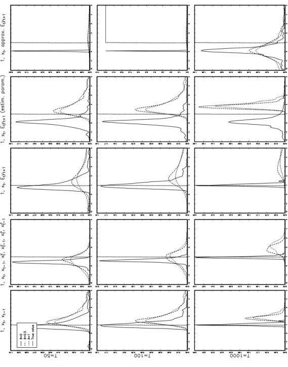
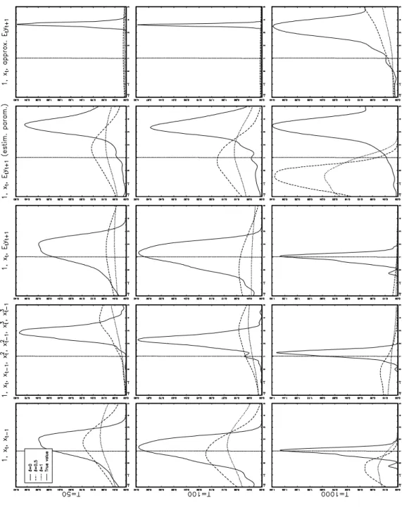
In the following simulations we vary four dimensions of the system: We have five choices for instrument sets; T = {50, 100, 1000}; δ = {0, 0.5, 1}; α is estimated freely or restricted between zero and one. Since the parameter δ takes the value zero, our simulations also cover the non-peso case, ie the standard linear case. The simulation results for non-restricted α are summarized in Figures 3–5. In each graph, a smoothed histogram, ie a kernel estimate of the empirical density function of the parameter estimator is computed. This is repeated for different values of the regime shift parameter δ = {0, 0.5, 1}. The sample size (T = {50, 100, 1000}) varies across the rows of the graphs and the instrument set (as described above) across the columns.

The empirical density functions of the estimator of the intercept term, ν, are presented in Figure 3. The GMM estimate is fairly precise in the absence of peso problem. The bias is also very small. However, in peso cases the bias may be substantial and uncertainties are large. In these cases the differences between instrument sets are small. It also seems that the use of polynomial instruments (instrument set 2) leads in many cases to marginally smaller biases than the use of other instrument sets.

The most interesting parameter is the discount factor, α. The empirical densities of its estimators are presented in Figure 4. Only in the standard linear case the median is within the feasible range α∈ (0,1). Even in such a case there is a high probability of estimating values above one. This demonstrates the failure of achieving a reasonable estimate of the discount factor in many applications of GMM to Euler equation estimation. In the peso case the results are very poor. The median is above one regardless of the choice of the instrument set. This is true even in the largest sample size, T = 1000. However, when the sample size is 50 or 100 and the polynomial instrument set is used, the median between zero and one is obtained. The variance of the estimator based on the polynomial instruments is also the smallest among the choices of instrument set. These features are not without cost: They are not preserved in the largest sample size; The bias of the GMM estimator of β is larger with the polynomial instrument set than with other instrument sets. The optimal instrument set (whether based on true or estimated parameter values) has undesirable properties. The variance is large and a major share of the probability mass is located in values above one. This finding is the same as reported by Tauchen (1986). However, the consistency of the optimal instrument is visible, particularly in the standard linear case: the larger the sample size the smaller the variance and the smaller the bias of the estimator.

The problem of obtaining estimates of α above unity might be due to the fact that the GMM estimator, as applied here, does not punish the objective function when the value of the discount factor exceeds unity. To overcome this problem the value of the discount factor may be fixed to an appropriate level or restricted, in course of optimization, into a feasible range.7 We experimented8 restricting the value of the discount factor between zero and one. This did not solve the problem since typically more than 50 per cent of the probability mass was placed on the (upper) boundary value.

The empirical densities of the estimator of ”the fundament effect”, ie the parameter β, are reported in Figure 5. The poor performance of the GMM

estimator is demonstrated also here. The peso problem leads to a very high variance of the GMM estimator compared to the standard linear case. In the standard, non-peso case, the use of the polynomial instrument set leads to an estimator with a low variance. However, the bias increases substantially. Note that contrary to the other sets this instrument set contains more instruments than the number of parameters. Consequently, this finding corresponds to that of Tauchen (1986): The larger the number of instruments the smaller the variance of the estimator but the larger the bias. The performance of the optimal instruments is statisfactory in the non-peso case.

The results concerning the peso cases are generally not improved when the value of the parameter α is restricted to lie between zero and one. In the peso cases the GMM estimator of β has still undesirable properties. The median is very much higher than the true value. Even the first percentile is above unity. There is, however, one interesting exception: In the standard linear case, the variance of the estimator of β is very low compared to the situation where the value of α is not restricted. Hence, the estimation of parameter β could benefit of restricting the discount factor, α. However, the bias is not a monotonic function of the sample size.

The poor small sample properties of the GMM estimators are not due to the poor choice of model. To measure the goodness of fit, we study the ratio between the variance of the expectational error ut≡ –α(yt+1 – Etyt+1) and the variance of yt.9

This variance ratio depends only on the values of the parameters of the system. Our choice of parameter values implies the value 0.25 of this ratio10 in the linear case.

We may summarize the simulation results as follows: First of all, the small sample properties of the GMM estimator – as applied here – are generally poor. It may even be possible that the estimator does not have finite moments for any finite sample size.11 A second feature is that it is very difficult to estimate the discount factor, α, even in the very simple linear case. This might explain results of many empirical studies where GMM is applied to Euler equation estimation: The value of the discount factor is usually fixed. The simulations illustrate that one cannot only blame a wrong model, but rather the estimation method. The restricted estimation leaks the problem into the estimates of parameter β. The third, slightly promising, feature is that the use of polynomial instruments might marginally improve the generally hopeless results.

9 _{Note that the multiple correlation coefficient is based on the same variance ratio, R}2 _{= 1 –}

Var(ut)/Var(yt).

10 _{This value corresponds R}2 _{= 0.75. Note, however, that in these models R}2 _{can be negative}

because yt+1 and ut can be (negatively) correlated.

11 _{The existence of moments of instrumental variable estimators attracted research up to early}

1980s. The main results are summarized, eg, in Davidson–MacKinnon (1993) and Judge et al. (1985). In the case of two-stage least squares, it is known that the number of finite moments (in finite sample sizes) is one less than the number of instruments minus the number of explanatory variables. Hence, in the case when the number of instruments equals the number of explanatory variables, no finite moments exists.

Figure 3. Estimated Density of GMM Estimator of ν Based on 500 Draws

The true parameter values are ν = 0, α = 1/1.05, β = 1, T = {50, 100, 1000}, µ = 0, φ1 = 1.1, φ2 =

–0.28 (the roots are 0.7 and 0.4), δ = {0, 0.5, 1}, c = 0.193 and σ2 = 0.001. The instruments sets vary across columns and sample sizes across rows. Monte Carlo simulations are based on 500 draws on normal distribution.

Figure 4. Estimated Density of GMM Estimator of α Based on 500 Draws

The true parameter values are ν = 0, α = 1/1.05, β = 1, T = {50, 100, 1000}, µ = 0, φ1 = 1.1, φ2 =

–0.28 (the roots are 0.7 and 0.4), δ = {0, 0.5, 1}, c = 0.193 and σ2 = 0.001. The instruments sets vary across columns and sample sizes across rows. Monte Carlo simulations are based on 500 draws on normal distribution.

Figure 5. Estimated Density of GMM Estimator of β Based on 500 Draws

The true parameter values are ν = 0, α = 1/1.05, β = 1, T = {50, 100, 1000}, µ = 0, φ1 = 1.1, φ2 =

–0.28 (the roots are 0.7 and 0.4), δ = {0, 0.5, 1}, c = 0.193 and σ2 = 0.001. The instruments sets vary across columns and sample sizes across rows. Monte Carlo simulations are based on 500 draws on normal distribution.

Table 1. Descriptive Statistics when α is not Restricted, Parameter ν Sample size Instru-ment set δ True value

Median Mean Std. dev. Biasa _RMSEb _Biasc _MADd

50 50 50 50 50 50 50 50 50 50 50 50 50 50 50 100 100 100 100 100 100 100 100 100 100 100 100 100 100 100 1000 1000 1000 1000 1000 1000 1000 1000 1000 1000 1000 1000 1000 1000 1000 1 2 3 4 5 1 2 3 4 5 1 2 3 4 5 1 2 3 4 5 1 2 3 4 5 1 2 3 4 5 1 2 3 4 5 1 2 3 4 5 1 2 3 4 5 0 0 0 0 0 0.5 0.5 0.5 0.5 0.5 1 1 1 1 1 0 0 0 0 0 0.5 0.5 0.5 0.5 0.5 1 1 1 1 1 0 0 0 0 0 0.5 0.5 0.5 0.5 0.5 1 1 1 1 1 0.000 0.000 0.000 0.000 0.000 0.000 0.000 0.000 0.000 0.000 0.000 0.000 0.000 0.000 0.000 0.000 0.000 0.000 0.000 0.000 0.000 0.000 0.000 0.000 0.000 0.000 0.000 0.000 0.000 0.000 0.000 0.000 0.000 0.000 0.000 0.000 0.000 0.000 0.000 0.000 0.000 0.000 0.000 0.000 0.000 0.0060 0.0030 0.0060 0.0020 0.0018 –0.4002 0.2959 –0.4343 –0.4002 –0.3430 –0.9077 0.6887 –0.8934 –0.9077 –0.9476 0.0088 0.0051 0.0088 0.0021 0.0021 –0.4537 0.0534 –0.8614 –0.4537 –0.7170 –1.0760 0.1161 –2.3730 –1.0760 –2.3130 0.0101 0.0093 0.0101 0.0026 0.0026 –0.5500 –0.5760 –1.7240 –0.5500 0.6296 –1.2710 –1.5590 –4.9940 –1.2710 1.3420 0.0055 0.0035 0.0055 0.0044 0.0020 –0.3780 0.3149 –11.4700 –0.3780 –16.6800 –1.1210 0.8315 –18.7600 –1.1210 –1.5420 0.0075 0.0064 0.0075 0.0042 0.0024 –0.3008 0.0790 –2.0970 –0.3008 5.8600 –2.5140 0.2309 –2.7290 –2.5140 –5.2880 0.0101 0.0093 0.0101 0.0062 0.0026 –0.5766 –0.5853 –3.3910 –0.5766 0.5821 –1.3530 –1.5080 –6.5220 –1.3530 2.0380 0.1598 0.0161 0.1598 0.0558 0.0084 6.9460 0.4408 267.6000 6.9460 204.9000 12.6700 1.1850 339.4000 12.6700 74.6600 0.0718 0.0126 0.0718 0.0427 0.0050 9.5560 0.5075 93.9100 9.5560 84.9500 33.9000 1.2790 54.1800 33.9000 90.8800 0.0043 0.0040 0.0043 0.0794 0.0155 0.1971 0.3162 24.4100 0.1971 7.1660 0.5015 0.8179 9.2720 0.5015 21.3800 0.0055 0.0035 0.0055 0.0044 0.0020 –0.3780 0.3149 –11.4700 –0.3780 –16.6800 –1.1210 0.8315 –18.7600 –1.1210 –1.5420 0.0075 0.0064 0.0075 0.0042 0.0024 –0.3008 0.0790 –2.0970 –0.3008 5.8600 –2.5140 0.2309 –2.7290 –2.5140 –5.2880 0.0101 0.0093 0.0101 0.0062 0.0026 –0.5766 –0.5853 –3.3910 –0.5766 0.5821 –1.3530 –1.5080 –6.5220 –1.3530 2.0380 0.1598 0.0161 0.1598 0.0558 0.0084 6.9460 0.4408 267.6000 6.9460 204.9000 12.6700 1.1850 339.4000 12.6700 74.6600 0.0718 0.0126 0.0718 0.0427 0.0050 9.5560 0.5075 93.9100 9.5560 84.9500 33.9000 1.2790 54.1800 33.9000 90.8800 0.0043 0.0040 0.0043 0.0794 0.0155 0.1971 0.3162 24.4100 0.1971 7.1660 0.5015 0.8179 9.2720 0.5015 21.3800 0.0060 0.0030 0.0060 0.0020 0.0018 –0.4002 0.2959 –0.4343 –0.4002 –0.3430 –0.9077 0.6887 –0.8934 –0.9077 –0.9476 0.0088 0.0051 0.0088 0.0021 0.0021 –0.4537 0.0534 –0.8614 –0.4537 –0.7170 –1.0760 0.1161 –2.3730 –1.0760 –2.3130 0.0101 0.0093 0.0101 0.0026 0.0026 –0.5500 –0.5760 –1.7240 –0.5500 0.6296 –1.2710 –1.5590 –4.9940 –1.2710 1.3420 0.0218 0.0091 0.0218 0.0068 0.0056 0.4663 0.3341 1.1980 0.4663 1.0830 1.0840 0.8038 2.9580 1.0840 3.2670 0.0134 0.0076 0.0134 0.0046 0.0034 0.4567 0.2845 1.3060 0.4567 1.6140 1.1020 0.7555 3.8000 1.1020 4.3730 0.0101 0.0093 0.0101 0.0033 0.0032 0.5499 0.5795 1.7240 0.5499 0.7324 1.2710 1.5530 4.9980 1.2710 1.6400

a_{Mean – true value} b_{Root mean square error} c_{Median – true value}

Table 2. Descriptive Statistics when α is not Restricted, Parameter α Sample size Instru-ment set δ True value

Median Mean Std. dev. Bias RMSE Bias MAD 50 50 50 50 50 50 50 50 50 50 50 50 50 50 50 100 100 100 100 100 100 100 100 100 100 100 100 100 100 100 1000 1000 1000 1000 1000 1000 1000 1000 1000 1000 1000 1000 1000 1000 1000 1 2 3 4 5 1 2 3 4 5 1 2 3 4 5 1 2 3 4 5 1 2 3 4 5 1 2 3 4 5 1 2 3 4 5 1 2 3 4 5 1 2 3 4 5 0 0 0 0 0 0.5 0.5 0.5 0.5 0.5 1 1 1 1 1 0 0 0 0 0 0.5 0.5 0.5 0.5 0.5 1 1 1 1 1 0 0 0 0 0 0.5 0.5 0.5 0.5 0.5 1 1 1 1 1 0.952 0.952 0.952 0.952 0.952 0.952 0.952 0.952 0.952 0.952 0.952 0.952 0.952 0.952 0.952 0.952 0.952 0.952 0.952 0.952 0.952 0.952 0.952 0.952 0.952 0.952 0.952 0.952 0.952 0.952 0.952 0.952 0.952 0.952 0.952 0.952 0.952 0.952 0.952 0.952 0.952 0.952 0.952 0.952 0.952 0.9160 0.3951 0.9160 0.1097 0.0690 1.5520 0.5897 1.6430 1.5520 1.5100 1.6290 0.4982 1.6080 1.6290 1.7370 1.0080 0.5743 1.0080 0.1435 0.0700 1.6640 0.8910 2.2100 1.6640 2.0540 1.7390 0.9208 2.6430 1.7390 2.6370 0.9966 0.9070 0.9966 0.1076 0.1151 1.7790 1.8220 3.4880 1.7790 0.1034 1.9050 2.1100 4.5580 1.9050 0.0489 1.3590 0.3781 1.3590 0.1372 0.0688 1.4930 0.5345 18.1600 1.4930 22.3500 1.7780 0.3928 13.9700 1.7780 1.9530 1.2040 0.5925 1.2040 –0.0818 0.0701 1.4440 0.8912 4.3210 1.4440 –6.6090 2.7920 0.8218 2.9150 2.7920 4.6000 1.0230 0.9181 1.0230 0.6631 0.1463 1.8250 1.8380 5.7590 1.8250 0.1693 1.9650 2.0740 5.6230 1.9650 –0.4388 7.2420 0.2171 7.2420 2.5980 0.0397 10.2000 0.6283 396.5000 10.2000 247.6000 8.7380 0.8494 232.1000 8.7380 50.2200 2.3280 0.1992 2.3280 3.8760 0.0257 13.3800 0.7029 134.7000 13.3800 113.2000 25.5700 0.9179 38.4700 25.5700 66.4500 0.1275 0.1037 0.1275 10.6400 2.1100 0.2743 0.4477 33.5300 0.2743 10.0100 0.3550 0.5800 6.5400 0.3550 15.0500 0.4065 –0.5743 0.4065 –0.8151 –0.8835 0.5411 –0.4179 17.2000 0.5411 21.3900 0.8260 –0.5596 13.0200 0.8260 1.0010 0.2515 –0.3599 0.2515 –1.0340 –0.8822 0.4920 –0.0611 3.3690 0.4920 –7.5610 1.8400 –0.1306 1.9630 1.8400 3.6470 0.0703 –0.0343 0.0703 –0.2893 –0.8061 0.8729 0.8858 4.8060 0.8729 –0.7831 1.0130 1.1220 4.6700 1.0130 –1.3910 7.2420 0.2171 7.2420 2.5980 0.0397 10.2000 0.6283 396.5000 10.2000 247.6000 8.7380 0.8494 232.1000 8.7380 50.2200 2.3280 0.1992 2.3280 3.8760 0.0257 13.3800 0.7029 134.7000 13.3800 113.2000 25.5700 0.9179 38.4700 25.5700 66.4500 0.1275 0.1037 0.1275 10.6400 2.1100 0.2743 0.4477 33.5300 0.2743 10.0100 0.3550 0.5800 6.5400 0.3550 15.0500 –0.0363 –0.5572 –0.0363 –0.8427 –0.8834 0.5997 –0.3627 0.6908 0.5997 0.5572 0.6764 –0.4542 0.6551 0.6764 0.7843 0.0556 –0.3780 0.0556 –0.8089 –0.8824 0.7114 –0.0614 1.2570 0.7114 1.1020 0.7868 –0.0316 1.6910 0.7868 1.6850 0.0442 –0.0454 0.0442 –0.8448 –0.8373 0.8266 0.8696 2.5350 0.8266 –0.8490 0.9522 1.1580 3.6060 0.9522 –0.9035 0.3208 0.5561 0.3208 0.8595 0.8833 0.7146 0.4570 1.7640 0.7146 1.5860 0.8145 0.5553 2.1480 0.8145 2.3820 0.2097 0.3790 0.2097 0.8613 0.8822 0.7136 0.4080 1.8610 0.7136 2.3720 0.8106 0.5274 2.8230 0.8106 3.1540 0.0747 0.0795 0.0747 0.8779 0.8795 0.8286 0.8716 2.5360 0.8286 1.0100 0.9524 1.1580 3.6200 0.9524 1.1310

Table 3. Descriptive Statistics when α is not Restricted, Parameter β Sample size Instru-ment set δ True value

Median Mean Std. dev. Bias RMSE Bias MAD

50 50 50 50 50 50 50 50 50 50 50 50 50 50 50 100 100 100 100 100 100 100 100 100 100 100 100 100 100 100 1000 1000 1000 1000 1000 1000 1000 1000 1000 1000 1000 1000 1000 1000 1000 1 2 3 4 5 1 2 3 4 5 1 2 3 4 5 1 2 3 4 5 1 2 3 4 5 1 2 3 4 5 1 2 3 4 5 1 2 3 4 5 1 2 3 4 5 0 0 0 0 0 0.5 0.5 0.5 0.5 0.5 1 1 1 1 1 0 0 0 0 0 0.5 0.5 0.5 0.5 0.5 1 1 1 1 1 0 0 0 0 0 0.5 0.5 0.5 0.5 0.5 1 1 1 1 1 1.000 1.000 1.000 1.000 1.000 1.000 1.000 1.000 1.000 1.000 1.000 1.000 1.000 1.000 1.000 1.000 1.000 1.000 1.000 1.000 1.000 1.000 1.000 1.000 1.000 1.000 1.000 1.000 1.000 1.000 1.000 1.000 1.000 1.000 1.000 1.000 1.000 1.000 1.000 1.000 1.000 1.000 1.000 1.000 1.000 1.3560 2.8650 1.3560 3.5410 3.6500 1.0120 4.4080 0.9436 1.0120 1.3340 1.5650 6.2890 1.9000 1.5650 1.2060 1.0290 2.2300 1.0290 3.4260 3.6000 0.1022 3.0450 –1.6570 0.1022 –1.3210 0.1039 4.4010 –3.9380 0.1039 –3.8270 0.9967 1.2530 0.9967 3.4400 3.4350 –0.6619 –0.7828 –7.3260 –0.6619 5.9470 –1.1230 –2.0830 –15.3000 –1.1230 8.8110 0.3724 2.8840 0.3724 3.5060 3.6560 0.6637 4.6940 –142.4000 0.6637 –53.0200 0.7685 7.6140 –85.9300 0.7685 5.9110 0.4972 2.1950 0.4972 3.9670 3.5990 1.5540 3.1590 –2.1710 1.5540 33.7700 –4.7910 4.8900 –3.5380 –4.7910 –21.1500 0.9307 1.2200 0.9307 1.9420 3.3550 –0.8179 –0.8681 –17.2200 –0.8179 5.5510 –1.4500 –2.0690 –21.3600 –1.4500 11.6500 20.2600 0.5779 20.2600 6.6810 0.1576 27.6200 2.5670 3340.0000 27.6200 552.0000 46.4700 5.5500 1630.0000 46.4700 219.3000 6.3970 0.5721 6.3970 9.8360 0.0939 61.9600 3.0980 543.3000 61.9600 506.2000 113.5000 5.1730 230.1000 113.5000 334.2000 0.3562 0.2897 0.3562 29.1500 5.8080 1.1670 1.8700 145.3000 1.1670 43.0200 1.9490 3.2060 35.5000 1.9490 80.8800 –0.6276 1.8840 –0.6276 2.5060 2.6560 –0.3363 3.6940 –143.4000 –0.3363 –54.0200 –0.2315 6.6140 –86.9300 –0.2315 4.9110 –0.5028 1.1950 –0.5028 2.9670 2.5990 0.5535 2.1590 –3.1710 0.5535 32.7700 –5.7910 3.8900 –4.5380 –5.7910 –22.1500 –0.0693 0.2204 –0.0693 0.9416 2.3550 –1.8180 –1.8680 –18.2200 –1.8180 4.5510 –2.4500 –3.0690 –22.3600 –2.4500 10.6500 20.2600 0.5779 20.2600 6.6810 0.1576 27.6200 2.5670 3340.0000 27.6200 552.0000 46.4700 5.5500 1630.0000 46.4700 219.3000 6.3970 0.5721 6.3970 9.8360 0.0939 61.9600 3.0980 543.3000 61.9600 506.2000 113.5000 5.1730 230.1000 113.5000 334.2000 0.3562 0.2897 0.3562 29.1500 5.8080 1.1670 1.8700 145.3000 1.1670 43.0200 1.9490 3.2060 35.5000 1.9490 80.8800 0.3561 1.8650 0.3561 2.5410 2.6500 0.0121 3.4080 –0.0564 0.0121 0.3339 0.5655 5.2890 0.8997 0.5655 0.2062 0.0291 1.2300 0.0291 2.4260 2.6000 –0.8978 2.0450 –2.6570 –0.8978 –2.3210 –0.8961 3.4010 –4.9380 –0.8961 –4.8270 –0.0033 0.2532 –0.0033 2.4400 2.4350 –1.6620 –1.7830 –8.3260 –1.6620 4.9470 –2.1230 –3.0830 –16.3000 –2.1230 7.8110 1.0740 1.8650 1.0740 2.6160 2.6510 1.8530 3.4130 4.0990 1.8530 5.0260 3.2230 5.3270 7.6130 3.2230 9.1490 0.7271 1.2310 0.7271 2.4770 2.6000 1.5270 2.3020 5.2070 1.5270 7.3470 2.4840 3.9060 10.7700 2.4840 12.6100 0.1946 0.2825 0.1946 2.5450 2.5540 1.6600 1.8350 8.3190 1.6600 5.3150 2.1230 3.2300 16.3300 2.1230 8.4360

7

Conclusions

This paper formalizes the concept of peso problem in terms of a linear Euler equation and a nonlinear marginal model. It turns out that the threshold autoregressive model as a marginal model is able to produce time-varying premia – contrary to the widely applied markov switching model. However, due to a nonlinear marginal model, there is no closed form solution to the system of equations. We discuss possible choices of computing the discounted sum of conditional future expectations of the marginal model.

Two estimation strategies emerge. The maximum likelihood is one possibility, but it leads to the numerical approximation of the conditional expectations of the marginal model. This is computationally burdensome and we can not give any Monte Carlo results of the properties of the ML estimator. The second choice is to apply GMM directly to Euler equation estimation. A clear advantage is that no assumption of the marginal model needs to be done. However, the simulation experiments illustrate that the GMM estimator, as applied here, has poor small sample properties in general and particularly so in the peso case.

The main problem with GMM lies in the estimation of the discount factor. The standard way to apply GMM to Euler equation estimation does not punish the GMM criteria when the discount factor gets unfeasible values, eg, values above unity. According to our simulations restricting the discount factor to lie between zero and unity does not solve the problem. The boundary value is attained in more than half of the cases. Improvements in the parameter β are marginal and concern only the non-peso case.

Appendix

Justification of equations (3.8a) and (3.8b)

First note that, for j = 2, (3.8a) and (3.8b) follow directly from (3.5) and (3.6). Now suppose that these equations hold for j ≥ 3 and observe that

. dx ) z ( p ) z ( k e dz ) z ( p ) z ( K A dz ) z ( p ) z ( K ) X ( K t 1 t t 1 t t 1 t X X j 1 X X 1 j X X j t 1 j + + +

∫

∫

∫

Here the first equality is based on (3.4) The second one follows from the induction assumption and the fact that, similarly to (3.5), also (3.6) and (3.8) hold even if Xt is replaced by z. By (3.6) the first term is the last expression equals

AKj(Xt). As for the second one, notice that, conditional on Xt, the first component

of Xt+1 has the density function g(z1−e1′h(Xt)) while the remaining components have a degenerate distribution at [xt … xt−p+2]′. Thus, the last integral equals

) X ( k dx )) X ( h e z ( g ) x ,..., x , z ( kj 1 t t−p+2 1 1 t 1 j+1 t ∞ ∞ − = ′ −

∫

References

Abel, A.B. (1982) Dynamic Effects of Permanent and Temporary Tax Policies in a q

Model of Investments. Journal of Monetary Economics 9, 353–373.

Baker, C.T.H. (1977) The Numerical Treatment of Integral Equations. Claredon Press. Oxford

Cagan, P. (1956) The Monetary Dynamics of Hyperinflation. In M. Friedman, ed., Studies in the quantity theory of money. Chicago, University of Chicago Press. Clements, M.P. − Smith, J. (1997) The Performance of Alternative Forecasting

Methods for SETAR Models. International Journal of Forecasting 13, 463−475. Davidson, R. – MacKinnon, J.C. (1993) Estimation and Inference in

Econometrics. Oxford University Press, Oxford.

Hall, R.E. (1978) Stochastic Implications on the Life Cycle-Permanent Income

Hypothesis Theory and Evidence. Journal of Political Economy 86, 971–588.

Hamilton, J.D. (1993) Estimation, Inference and Forecasting of Time Series Subject

to Changes in Regime. In G.S. Maddala, C.R. Rao and H.D. Vinod, eds., Handbook

of Statistics. Vol. 11, New York, North-Holland.

Hamilton, J.D. (1994) Time Series Analysis. Princeton University Press, Princeton. Hansen, B.E. (1996) Inference when a Nuisance Parameter is not Identified under

the Null Hypothesis. Econometrica 64, 413−430.

Judge, G.G. –Griffiths, W.E. – Hill, R.C. – Lütkepohl, H. – Lee, T.C. (1985) The Theory and Practice of Econometrics. Second Edition. John Wiley and Sons, New York.

Masry, E. − Tjøstheim (1995) Nonparametric Estimation and Identification of

Nonlinear ARCH Time Series: Strong Convergence and Asymptotic Normality.

Econometric Theory 11, 258−299.

Newey, W.K. (1993) Efficient Estimation of Models with Conditional Moment

Restrictions. In G.S. Maddala, C.R. Rao and H.D. Vinod, eds., Handbook of

Statistics. Vol. 11, New York, North-Holland.

Tauchen, G. (1986) Statistical Properties of Generalized Method of Moments

Estimators of Structural Parameters Obtained from Financial Market Data.

Journal of Business & Economic Statistics 4, 397−425.

Tong, H. (1990) Non-Linear Time Series. A Dynamic System Approach. Claredon Press, Oxford.