Wayne State University Civil and Environmental Engineering Faculty
Research Publications Civil and Environmental Engineering
4-26-2016
Evaluation of Alternative Implementation Methods
of Failure Sampling Approach for Structural
Reliability Analysis
Kapil PatkiWayne State University, [email protected]
Christopher D. Eamon
Wayne State University, [email protected]
Recommended Citation
Patki, K., & Eamon, C. (2016). Evaluation of Alternative Implementation Methods of a Failure Sampling Approach for Structural
Reliability Analysis.ASCE-ASME Journal of Risk and Uncertainty in Engineering Systems, Part A: Civil Engineering, 2(4), 04016004.
doi:10.1061/AJRUA6.0000876
Evaluation of Alternative Implementation Methods of Failure Sampling Approach for Structural Reliability Analysis
Kapil Patki1 and Christopher Eamon2
Abstract
In this paper, several alternative approaches are used to implement the failure sampling method for structural reliability analysis and are evaluated for effectiveness. Although no theoretical limitation exists as to the types of problems that failure sampling can solve, the method is most competitive for problems that cannot be accurately solved with reliability index-based approaches and for which simulation is needed. These problems tend to have non-smooth limit state boundaries or are otherwise highly nonlinear. Results from numerical integration and three extrapolation approaches using the generalized lambda distribution, Johnson's distribution, and generalized extreme value distribution are compared. A variety of benchmark limit state functions were considered for evaluation where the
number of random variables, degree of non-linearity, and level of variance were varied. In addition, special limit state functions as well as two complex engineering problems requiring nonlinear finite element analysis for limit state function evaluation were considered.
It was found that best results can be obtained when failure sampling is implemented with an extrapolation technique using Johnson's distribution, rather than with numerical integration or the generalized lambda distribution as originally proposed with the method.
---
1. PhD Student, Dept. of Civil & Environmental Engineering, Wayne State University, Detroit, MI 48202; [email protected].
2. Associate Professor of Civil and Environmental Engineering, Wayne State University, Detroit, MI 48202; [email protected]
Introduction
Reliability analysis of complex engineering problems, such as those requiring finite element analysis, often demand high computational costs. Both simulation-based methods, such as Monte Carlo Simulation (MCS) and its variants, as well as reliability index
approaches such as the First Order Reliability Method (FORM), have been popular choices for structural reliability analysis. FORM and similar methods such as the Second Order Reliability Method (SORM) (Rackwitz and Fiessler 1978; Breitung 1984) rely on identifying the most probable point of failure (MPP) on the failure boundary. Reliability index 𝛽 is commonly used in structural reliability analysis to quantify structural safety rather than failure probability directly. It is usually calculated as the distance between the MPP and the origin in standard normal space, where the MPP represents the location of the largest value of the joint probability density function that lies upon the failure boundary of the limit state function. Although computationally efficient, these methods may provide poor solutions for problems nonlinear in standard normal space caused by the linearization of the limit state function at the MPP (Eamon et al. 2005; Melchers 1999; Chiralaksanakul and Mahadevan 2005; Haldar and Mahadevan 2000). Moreover, search algorithms sometimes cannot identify the MPP for complex problems that may be highly non-linear, discontinuous, or that have multiple ‘local’ MPPs on the failure boundary (Eamon and Charumas 2011). In such cases, if the MPP cannot be found, the reliability index-based methods will fail to provide any
solution.
To reduce the cost of simulation methods but maintain reasonable accuracy, numerous variance reduction techniques were developed such as stratified sampling (Iman and Conover 1982), importance sampling (Rubinstein 1981; Engelund and Rackwitz 1993) and adaptive importance sampling (Wu 1992; Karamchandani et al. 1989). However, stratified sampling
significant reductions in computational costs; and as importance sampling methods also rely on identifying the MPP, they may also fail to provide solutions, or provide poor solutions, for complex limit states. Various other simulation methods that do not rely upon the MPP have been proposed, such as subset simulation (Au and Beck 2001; Au et al. 2007) and directional simulation (Ditlevesen and Bjerager 1988), among many others. Although directional simulation can perform extremely well in some cases, such as when the limit state boundary approaches a spherical shape, it is not particularly efficient when the boundary takes a planar form or small multiples thereof (Engelund and Rackwitz 1993). A significant body of research has been conducted on the development of subset simulation methods, and multiple competing versions exist. An important consideration with this method, however, is proper selection of the importance sampling density, some choices of which can be associated with high variance in the solution (Au and Beck 2001; Au et al. 2007).
Alternatively, rather than refine the reliability method, a response surface technique can be used to represent a computationally expensive limit state function with a simpler, analytical surrogate function (Gomes and Awruch 2004; Cheng and Li 2009). Once formed, the response surface can be used to provide very fast reliability solutions. However, these techniques often require high computational effort to develop accurate responses for highly non-linear or discontinuous limit state functions, a cost which may outweigh the savings gained with their use (Eamon and Charumas 2011).
As an alternative solution for complex reliability problems, this paper examines the use of a modified conditional expectation approach proposed by Eamon and Charumas (2011), 'failure sampling.’ The method was reportedly used to accurately solve various complex limit states with reasonable computational effort. The approach offers several useful features: (1) as there is no reliance on the MPP, complex problems for which the MPP cannot be accurately located, and thus are unsolvable or poorly solved by methods such as
FORM, SORM and importance sampling, can be addressed; (2) for many complex, moderate reliability (i.e. reliability index from 3-5) problems that are poorly solved with many other methods, computational effort for failure sampling is relatively low; (3) efficiency does not vary significantly among different types of problems of the same reliability level; and (4) the method is mathematically simple and straightforward to implement.
It should be emphasized that, as a simulation-based method, although it can be theoretically applied to problems of any complexity or reliability level, failure sampling is most effective for problems that are complex and for which reliability index-based methods provide no or poor solutions, and for which other simulation methods require an unfeasibly large computational effort. For practical implementation, two observations can be noted. First, earlier work, as well as the results of this study, have found that no more than 1000 simulations are usually sufficient to solve a wide range of complex problems with reliability indices from 3-5 and sometimes higher (Eamon and Charumas 2011). Increasing the number of simulations will correspondingly increase the precision of the solution as well as the reliability level that can be addressed. Second, for problems that can be solved accurately with non-simulation methods such as FORM (typically, problems that are simple; i.e. smooth limit state boundaries that are not highly nonlinear in standard normal space), failure
sampling is usually not competitive, as reliability index-based approaches can typically accurately solve simple problems with many fewer calls to the limit state function than can a simulation approach. Thus, for simpler problem types and for problems with low reliability, other methods are generally more efficient.
The failure sampling solution process can be implemented in various ways. In previous work, the numerical integration and generalized lambda distribution fit methods were used, which are described in the next section. In this study, several alternative methods
are considered, and results superior to those originally presented by Eamon and Charumas (2011) are identified.
Summary of Failure Sampling
The starting point for a conditional expectation solution is to construct a data sample of random variables (Xj) that only lies upon the failure boundary of a limit state function g(Xj). This is achieved by simulating values of all random variables except one (Q) (call this
remaining, realized set of random variables (xi)), then determining the value q that sets g = 0.
As the resulting complete set of (xj) (containing (xi) and q) is biased due to the non-random
values determined for Q, (xj) is not used to directly compute failure probability pf as with the
traditional MCS process (as this would always result in pf = 1.0). In the failure sampling
process, values for Q are not of interest; Q is a single random variable with statistical properties that are expected to be fully defined. Rather, assuming the problem has multiple random variables and is somewhat complex, a statistical description of the random function within g containing the variables other than Q, R(Xi), is of interest, which can be found by
obtaining values for Q, as described using the process below. The advantage of sampling
R(Xi) only rather than sampling g directly with all RVs (Xj), such as in the traditional MCS
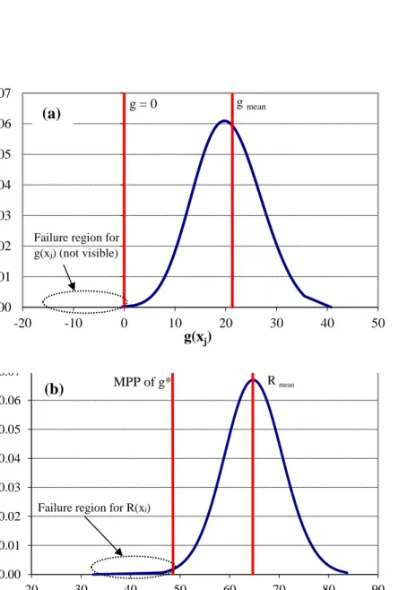
process, is significant. In particular, only sampling R(Xi) allows the failure region of the
problem to be more easily captured, as shown in Figure 1. The complete approach is fully described elsewhere (Eamon and Charumas 2011), whereas a step-wise summary of the procedure is provided here.
1. From an original limit state function g(Xj) with random variables (Xj), a control random
variable Q is chosen. A new limit state function g* is then formed such that it has an equivalent failure boundary to that of g(Xj), but Q is separated from the remaining random
g* = R(Xi) - Q = 0 (1)
Here, R(Xi) is the portion of the limit state function that is not a function of Q, and (Xi) is the
set of all random variables (Xj) except Q. There is no theoretical limitation to the selection of Q, although it is best that Q is selected such that it is statistically independent of the
remaining random variables (Xi). For example, consider a simple limit state function g = X1X2 - X3/X4. Assume X3is chosen as the control variable Q. A new limit state boundary is
then written as g* = 0 = X1X2X4 - X3. Here, X1X2X4 = R(Xi) and X3 = Q. In a more realistic,
complex case, g* can only be expressed implicitly, such as: g* = f(Xi, Q), where the
evaluation of f(Xi, Q) requires a numerical method such as finite element analysis. This
implicit form causes no theoretical difficulty, as g* need not be explicitly expressed in terms of (Xi) and Q. However, implicit forms of g* will require the use of a nonlinear solver to set g* = 0, as discussed in step 3 below.
2. Random values for variables within R, (Xi) (i.e. all random variables except Q) are
simulated. In this paper, direct MCS is used for the simulation. R(Xi) is then evaluated. For
the example above, MCS would be used to simulate values x1, x2, and x4 for random variables X1, X2, and X4, respectively.
3. Based on the set of realized random variable values (xi) in step 2, the value of Q needed to
satisfy Eq. 1, (q), is determined. For simple problems that can be written explicitly as g* = 0 = R(Xi) – Q, this is simply q = R(xi). For implicit, nonlinear problems, such as g* = f(R(Xi), Q), to find a value q such that g* = f(R(xi), q) = 0, no closed-form solution exists, and some
type of nonlinear solver must be used. In general, q is incrementally increased (or decreased) until the limit state g* equals zero. For this study, the bisection method is used with 1%-3%
tolerance to satisfy Eq. 1 for such problems, as discussed in more detail in example problem 3, below.
4. Steps 2-3 are repeated until a sufficient number of values for Q have been determined. In this paper, 1000 simulations were used. At this point, there is no need to evaluate the true response further. Notice that, since q = R(xi) per step 3, the values of q that were determined
also equal values of R(xi) on the failure boundary. That is, a data sample representing the
random function R(Xi) with variables (Xi) (i.e. all but Q) has been established.
5. The data sample for R(xj) is further manipulated in one of two ways. In the first process,
the numerical integration approach, a probability density function (PDF) estimate of the data is developed. This PDF is then numerically integrated to form a cumulative distribution function (CDF). As discussed in Eamon and Charumas (2011), rather than forming a CDF directly from the R(xi) data sample, developing a PDF first tends to reduce variance in the
solution. As recommended, when considering the integration approach, the PDF estimate was formed from 50 intervals, creating a 50-point CDF upon integration. The second method in which the R(xi) data can be manipulated is by replacing the data completely with an
analytical curve. If the curve is highly flexible and can fit the data well, this approach has the advantage of extending the tail of R(xi) beyond that which was originally generated.
6. Failure probability is estimated. Two general approaches exist, depending on the method used to manipulate the R(xi) data in step 5. Notice that, with the statistical parameters of R(Xi) estimated, the limit state function is effectively reduced to a two random variable
problem given by: g* = R – Q, where the potentially complex (and possibly implicit) R(Xi) is
Considering the first method for solution, if the numerical integration approach discussed in step 5 was used to form a CDF of R(xi), the most straightforward way to
compute pf is to simply numerically integrate the well-known expression:
In Eq. 2, FR(x) refers to the estimated CDF of R(xi), found per step 5, and fQ(x) is the PDF of Q.
Alternatively, if the original R(xi) data are represented with an analytical distribution, pf (or reliability index ) of g* = R – Q can be quickly calculated with one of many available
simple reliability methods, such as MCS or FORM, as the original, potentially complex multi-variate function g is now represented analytically as an equivalent, simple and
analytical two random variable problem with R and Q fully defined. With this approach, for this study, MCS was used to compute pf of g*, then results reported in terms of reliability
index with the transformation β= -Φ-1(pf), where Φ is the standard normal CDF. Notice
that essentially represents the number of standard deviations from the mean of a standard normal random variable associated with the given failure probability. Although
transformation from pf to β is not necessary, reliability index is the standard metric of safety
in structural reliability analysis rather than pf directly, which is often numerically
cumbersome. Note that typical notional reliability indices of components designed by prevailing structural engineering Load and Resistance Factor Design standards are generally between 2 and 4 (Rosowsky et al. 1994; Eamon and Nowak 2005; Szerszen and Nowak 2003)).
Implementation Methods Considered
Johnson’s distribution (JSD), and the generalized extreme value distribution (GEV). The generalized lambda distribution is a four parameter distribution known for its high flexibility, and can represent many common distributions such as normal, lognormal, Weibull, etc. (Karian and Dudewicz 2011). The distribution is defined by four parameters: λ1,
λ2, λ3, and λ4. Parameters λ1 and λ2 are location and scale parameters, respectively, while λ3
and λ4 describe skewness and kurtosis. The distribution can be defined as follows. Given the
quantile function 𝑄(𝑢) = 𝜆1+
𝑢𝜆3−(1−𝑢)𝜆4
𝜆2 (the inverse of the CDF), at x = Q(u), where
input parameter u refers to probability (i.e. from 0 to 1), the PDF of the generalized lambda distribution is given by:
𝑓𝑅(𝑥) = 𝜆2
[𝜆3𝑢(𝜆3−1)+ 𝜆
4(1 − 𝑢)(𝜆4−1)]
(3)
There are numerous methods to determine the parameters of the distribution (Karian and Dudewicz 2011; Ozaturk and Dale 1985; Asif and Helmut 2000). For this study, the method of moments was used (Karian and Dudewicz 2011). This process makes use of expressions that relate parameters λ1 -λ4 to the first four sample moments. However, these expressions are
implicit, and due to the algebraic complexity of the relationships, direct solution of λ1 -λ4 is
generally not possible, and numerical methods are commonly employed. In a typical
numerical process, values for λ3 and λ4 are first found by minimizing the difference between
the generalized lambda distribution moments and the sample moments, while constraining results to a feasible solution space. In this study, a sequential quadratic programing optimization technique is used to solve the minimization problem. Once λ3 and λ4 are
determined, the relationships among λ1 -λ4 and the sample moments described above can be
sufficiently simplified such that the remaining parameters λ1 and λ2 can be found
In some cases, changing the method used to determine the generalized lambda distribution curve parameters may influence the resulting quality of fit. In addition to the method of moments, other common methods of determining curve parameters for the generalized lambda distribution include the method of percentiles and the method of L-moments. Some have found that the method of percentiles gives superior results to the method of moments when sample moments are computed with higher levels of uncertainty; i.e. usually when considering small sample sets and large coefficients of variation (Karian and Dudewicz 2011). However, the authors of this study found no significant advantage with the method of percentiles over the method of moments for fitting the generalized lambda distribution to the problems considered. Although the method of L-moments has been shown to provide good results in some cases, it was generally found to produce inferior results for the generalized lambda distribution when compared to the method of percentiles (Karian and Dudewicz 2003), and was thus not considered further in this study.
Similar to the generalized lambda distribution, the Johnson system of distributions is defined by four parameters and has significant flexibility to cover a wide variety of shapes. The Johnson system is based on three possible transformations of a normal random variable in addition to the identity transformation. The ‘SB’ transformation represents a bounded distribution, the ‘SL’ transformation represents a semi-bounded distribution, and the ‘SU’ transformation represents an unbounded distribution in the Johnson system. Transformation from a standard normal random variable Z to a Johnson random variable X for the SB, SL and SU transformations can be represented as follows:
𝑋 = ξ + 𝜆𝑗∙ 𝛤−1(𝑍 − 𝛾
𝛿 ) (4)
where Γ denotes the transformation function, γandδ are the shape parameters, ξ is the location parameter, and λj is the scale parameter. The resulting PDF is given by:
𝑓𝑅(𝑥) = 𝛿 𝜆𝑗√2𝜋 𝑔′ (𝑥 − ξ 𝜆𝑗 ) 𝑒𝑥𝑝 [ −1 2(𝛾 + 𝛿 𝑔 ( 𝑥 − ξ 𝜆𝑗 ) ) 2 ] (5)
where g(y) = ln(y), ln(y/(1-y)), and ln(y+(y2+1)1/2) for the SL, SB, and SU transformations, respectively, and Y= (X- 𝜉) /𝜆𝑗 . The ‘SN’ transformation is the identity transformation and represents a normal distribution. Although various methods to determine the parameters of the Johnson distribution are available, the method of moments, method of percentiles, and method of quantile estimators are common. In this research, the method of percentile
estimators was used (Karian and Dudewicz 2011; George 2007; Slifker and Shapiro 1980), as it was found that the method of moments produced less accurate estimations of the third and fourth moment parameters for the Johnson distribution, particularly when the sample size becomes small. In the percentile method, specified percentiles of the standard normal distribution are matched with corresponding percentile estimates of the sample. More
specifically, using the process described by Slifker and Shapiro (1980), the parameters of the distribution are determined by solving the transformation function Γ at four different
percentiles, where the percentiles of the standard normal variate are taken between three intervals of equal length at points ±𝑧 and ± 3𝑧. Based on the calculated discriminant value between the percentiles, a best-fit Johnson family can be selected, and with explicit
expressions available in the literature (Slifker and Shapiro 1980), the corresponding distribution parameters are readily determined.
The generalized extreme value distribution combines three simpler distributions into a single form, allowing a continuous range of possible shapes weighted among the component distributions. Similar to the extreme value distribution, the generalized type is often used to model the smallest or largest values in a large set of independent data. It is defined by a location parameter μ, a scale parameter σ, and a shape parameter k, where k takes on a value other than zero. The PDF of the distribution is described by:
𝑓𝑅(𝑥) = 1 𝜎exp (− (1 + 𝑘 (𝑥 − 𝜇) 𝜎 ) −1 𝑘 ) ((1 + 𝑘(𝑥 − 𝜇) 𝜎 ) −1−1𝑘 ) (6)
The parameters of the distribution were determined using similar techniques as those used for the Johnson distribution.
Comparison Problems and Results
As noted in the introduction, the purpose of this study is to investigate the
effectiveness of different methods of implementing failure sampling, and perhaps to lead to additional improvements in method accuracy and/or efficiency. As such, it is desirable to investigate the performance of the implementation methods with a variety of different reliability problems. For such an evaluation to be feasible, the true solution of the problems must be readily verifiable. Therefore, some of the problems investigated are benchmark reliability problems taken from the literature. As established benchmark problems, these can be effectively solved with existing reliability approaches, and a failure sampling solution is not needed, nor does it represent the most efficient solution for some of these problems. Nevertheless, the solution of such problems can provide valuable information as to the effectiveness of the investigated implementation approaches for different problem types. However, as failure sampling was specifically intended for complex, more realistic
engineering problems, two problems of this type were also considered, both of which involve nonlinear finite element analysis for the evaluation of the limit state function (problems 3 and 4). In order to identify potential differences in the implementation methods, a relatively small number of simulations (1000) was used to solve all problems, even those with a reliability index approaching 4 (pf approximately 1:30,000). Although very reasonable
indices, if desired, additional accuracy and precision can be achieved by increasing the number of simulations.
Problem Series 1: Flexible Limit State Function
This function is taken from Eamon et al. (2005) and is used to evaluate the effect of varying the number of random variables (RVs), distribution type, level of variance, problem linearity, and target reliability level. Specific parametric variations included: 2, 5, and 15 RVs; coefficients of variation of 5% and 35%; normal, lognormal, and extreme type I distributions; algebraic linearity, where linear, moderately nonlinear, and highly nonlinear limit states were considered; and target reliability index, where ‘low’ and ‘high’ values were considered, ranging from 0.3 - 5.0. Various combinations of these different parameters resulted in a total of 72 different limit state functions for consideration. The general form of the limit state function is given as:
𝑔 = 𝑘 ∑ 𝑑𝑖 𝑛 𝑖=1 − 𝑐 ∑𝐿𝑗 4𝑤 𝑗 𝐸𝑗𝐼𝑗 𝑘 𝑗=1 (7)
Parameters taken as RVs are given in Table 1, while values for the parameters are given in Table 2, and have been used either as the mean value if an RV, or a constant value if a non-RV, depending on the case type. All cases were evaluated with failure sampling using numerical integration (abbreviated as “NI” in the figures and tables), and the generalized lambda, Johnson, and generalized extreme value distribution implementations. Results are measured in terms of accuracy and precision, where accuracy is the mean value of the ratio of computed reliability index to the exact value for the specific case under consideration. The exact value for low to moderate target reliability indices is determined from 1 x 10⁶ MCS simulations, and for high target reliability index cases, the exact value is determined from 1 x 10⁹ MCS simulations. Precision is used to measure the degree of consistency of results, and is
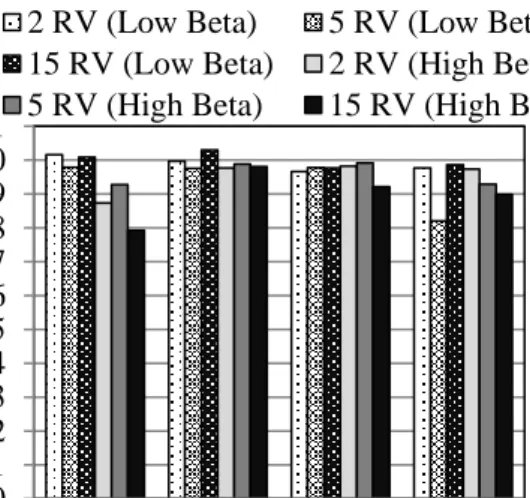
determined by calculating the coefficient of variation (COV) of accuracy, based on five evaluations of each problem. Figures 2-7 show the effect of number of RVs, degree of non-linearity, and RV distribution type on the different implementation methods.
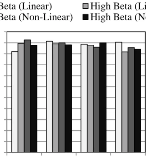
Figures 2 and 3 concern the effect of linearity. As shown, it was found that varying linearity had little effect on solution quality. Considering differences among methods, by a slight margin, the generalized lambda distribution produced the best overall results for
accuracy (Figure 2), generating error within 1% for all cases (where throughout this study, % error is taken as the absolute value of: (exact value – calculated) x 100 /exact value).
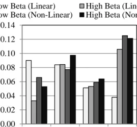
However, the Johnson distribution produced nearly the same results with the exception of one case (nonlinear, low reliability), at 4% error. Numerical integration and the generalized extreme value distribution provided less consistent accuracy from case to case, and the generalized extreme value distribution performed worse overall, with three cases from 5-8% error. For precision (Figure 3), the Johnson distribution generated best results overall, with only 5-6% COV in the solution when using 1000 simulations. The generalized lambda distribution was somewhat worse, with COV from 8-10%. Similar to the results for accuracy, numerical integration and the generalized extreme value distribution were most variable from case to case for precision, with the generalized extreme value distribution results again worse overall, with about 10-12% COV.
Generally, as shown in Figures 4 and 5, increasing the number of RVs also had no significant effect on solution outcome. However, the 15 RV, high reliability case was generally least precise for all methods. The generalized lambda and Johnson distributions produced nearly the same accuracy (Figure 4), with about 4% error or less for all cases. One exception is the 15 RV high reliability case, for which the Johnson distribution generated 7% error. Similar to previous results, numerical integration and the generalized extreme value
cases (5 RV, low reliability for the generalized extreme value distribution and 15 RV, high reliability for numerical integration), error approached a very high 20%. Regarding precision (Figure 5), the Johnson distribution was shown to produce best results overall, where COV ranged from 3-6% in all cases except one (15 RV, high reliability) and COV was approximately 10%. However, all other methods produced higher solution variance with this case as well, with COV from about 12-14%. The generalized lambda distribution performed worse overall for precision, ranging from about 12-15% COV. As with previous results, significant variation was found among cases with both numerical integration and the generalized extreme value distribution, ranging from 2-14% COV depending on problem type.
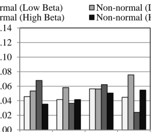
As with previous results, altering RV distribution normality, as shown in Figures 6 and 7, did not degrade the solution. As shown in Figure 6, only minor variations in accuracy were found among different methods. One exception is the normal, high reliability case, for which the Johnson distribution produced a relatively high error at about 9%. For precision (Figure 7), results were again similar for most methods, producing about 4-6% COV. Overall, the generalized lambda distribution appears best, with most cases at 4% COV. However, results from the Johnson distribution are more consistent among cases, though with a slightly higher typical COV at about 6%. As with some previous results, most variation from case to case occurred with numerical integration and the generalized extreme value distribution.
In summary, the results show that most implementation methods produced reasonably accurate results for most cases, though precision suffered in some cases when limiting the sample to 1000 simulations. In particular, the generalized extreme value distribution
demonstrated relatively poor precision for nonlinear limit states and for high reliability cases, while the generalized lambda distribution implementation lacked precision in general relative
to the other approaches. As expected, all methods were accompanied by a decrease in precision for high reliability cases with a high number of RVs. Though a few exceptions exist, overall, the most accurate and consistent results were found with the Johnson
distribution. Surprisingly, the cases where the Johnson distribution yielded lowest accuracy were linear limit state functions. However, these cases were those with 15 RVs and high beta values. It was also found that the precision of numerical integration, the generalized lambda distribution and the generalized extreme value distribution decreased most when the number of RVs increased. Here, the generalized lambda and generalized extreme value distributions failed to provide a good fit for highly non-linear cases with 15 RVs. For the generalized lambda distribution, this can be attributed to a poor representation of skewness and kurtosis of the distribution for the limited size of the R(xi) sample taken. The generalized extreme
value distribution, however, poorly represented the tail region.
Problem Series 2: Special Limit State Functions
Engelund and Rackwitz (1993) presented a series of unique, often difficult to solve limit state functions. The results of two of these functions found to be most challenging for the methods considered in this paper are presented below.
Multiple Reliability Indices:
This hyperbolic limit state function has two reliability indices, and is given as:
𝑔 = 𝑥1𝑥2 − 146.14 (8)
where x1 and x2 are normal RVs having mean values of 78064.4 and 0.0104, with
corresponding standard deviations of 11709.7 and 0.00156, respectively. Results are presented in Table 3, where it can be observed that only numerical integration and the Johnson distribution could produce results, whereas the generalized lambda and generalized
precision for numerical integration and the Johnson distribution are similar, with numerical integration slightly superior (exact solution obtained from 1 x 10⁹ MCS samples). For comparison, MCS and FORM solutions (limited to the same computational effort as the failure sampling approaches) are given as well; neither could produce a viable solution for this problem.
Maximum Function:
This limit state function is expressed as the maximum of several sub-functions, and is given by the following expression:
𝑔 = max(𝑔1, 𝑔2, 𝑔3,𝑔4) (9) where: 𝑔1= 2.677 − 𝑢1− 𝑢2 𝑔2= 2.500 − 𝑢2− 𝑢3 𝑔3= 2.323 − 𝑢3− 𝑢4 𝑔4= 2.250 − 𝑢4− 𝑢5
All ui are standard normal random variables. As with the previous example, as shown in
Table 4, the generalized lambda and generalized extreme value distributions were unable to fit the data, whereas numerical integration and the Johnson distribution produced reasonable results. In this case, the Johnson distribution produced the greatest accuracy and precision (exact solution obtained from 1 x 10⁹ MCS samples).
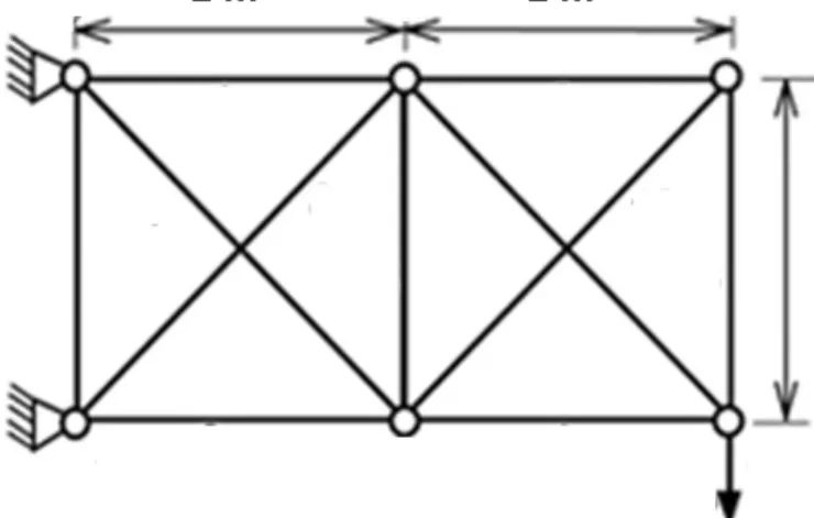
Problem 3: Non-Linear Truss
This problem is based on that described in Eamon and Charumas (2011), and is meant to represent complexity in the range of that for which the failure sampling approach is
finite element code (ABAQUS) was used to evaluate the response. Two different limit states were considered for this problem: one in terms of displacement, and another in terms of stress. The material was taken as steel, with a bilinear stress-strain curve and an elastic modulus E of 200 GPa (29,000 ksi). For the displacement-based limit state problem, only three RVs were considered: yield stress (σy), post-yield modulus (E2), and load (P). RVs σy
and E2 are considered to be the same for all truss members, with means of 345 MPa (50 ksi)
and 8.28 GPa (1200 ksi), and COVs of 0.10 and 0.25, respectively. To vary reliability index, two values of P were considered: 223 and 267 kN (50 and 60 kips), with COV of 0.10. A third variation of this problem was considered as well in which resistance RVs (σy, E2, P)
were taken as partially correlated (ρ= 0.50), and COV of each increased to 0.35. In all problems, failure is defined as the state where displacement at the point of load application exceeds 1.5 inches. Hence, the limit state function is given as:
g = 1.5 - D(σy, E2, P) (10)
All RVs are taken as normally distributed, and P was considered to be the control variable. The bisection method was used to solve for the condition g* = 0 (Eq. 1), with an error tolerance of 1% in one case and 3% in a second case, for comparison. The method works by bracketing the solution, then refining the solution estimate with subsequent linear
interpolations that narrow the bracket. Note that although the limit state function was evaluated with a sample size of 1000 (the "nominal" number of calls given in the results tables), the actual number of function calls (the "actual" number of calls given in the tables) exceeded this value, due to the iterative process needed to find the root of g* = 0 . More sophisticated root finding techniques are available that can decrease the actual number of calls further, improving solution efficiency. However, this is a topic beyond the scope of this paper. For fair comparison, the actual number of calls is kept constant for all methods, such
A more complex version of the problem was also considered, where the limit state function was reformulated in terms of stress. In this case, each member of the truss was associated with three independent RVs, resulting in a total of 31 RVs for the problem. RVs are cross-sectional area A (mean = 1290 mm2 (2 in2), COV = 0.05), and the previous RVs of yield stress σy and post yield modulus E2, with the same statistical parameters used in the
displacement problem. The mean value of load P (the control variable) was taken as 223 kN (50 kips) in one version of the problem and 289 kN (65 kips) in another, to vary target reliability index, with COV of 0.1. A third variation was also considered in which resistance RVs were taken as partially correlated (coefficient of correlation ρ= 0.30) for area RVs, yield stress RVs (ρ= 0.50), and for yield modulus RVs (ρ= 0.70), while the COV of the post-yield modulus RVs was increased to 0.30. The failure criterion was defined as the state where the stress in member 1 reaches its yield stress. The resulting limit state function is given as:
g =σy1 - σ1(P, σyj, E2i, Ai) for i = 1 to 10, j = 2 to 10 (11)
The exact solution was obtained from 1 x 10⁹ MCS samples, which required approximately 400 CPU hours. Tables 5 and 6 show the results obtained for the displacement and stress limit state functions, respectively. For comparison, and to verify the suitability of problem complexity, a FORM solution was also attempted. This resulted in relatively high errors or solution failure for the displacement problems (Table 5) and failed to provide solutions for the stress problems (Table 6), as the MPP could not be located. Similarly, no solution could be obtained from MCS for the higher reliability cases when limiting the actual number of function calls to that used by the failure sampling implementation methods.
For the displacement limit case (Table 5), all failure sampling implementation methods produced reasonable results (1-5% error) for the low reliability level case (P = 267 kN) except numerical integration, where error was approximately 9%. For the higher
reliability case (P = 223 kN), only numerical integration and the Johnson distribution could solve the problem, with similar, relatively low error from 2-3% for the high (3%) g* = 0 tolerance, and about 0.5% error for the low g* = 0 (1%) tolerance alternative. Of course, the higher accuracy associated with lower g* = 0 error tolerance is accompanied by higher simulation cost, which increased from 5000 to 8000 actual simulations, as shown. For the correlated, high COV RV case, the performance of numerical integration markedly
decreased, producing a large error of approximately 25%. However, the Johnson distribution solution was not significantly affected, producing less than 3% error.
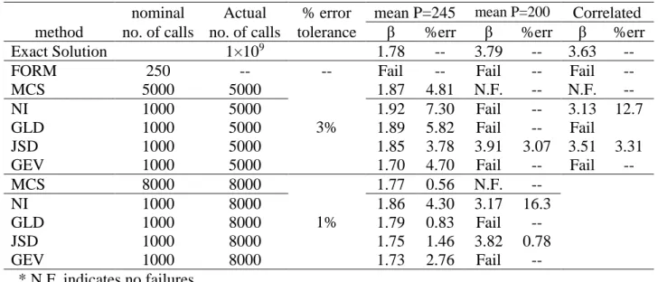
Considering the stress limit case (Table 6), as with the previous displacement limit problem, all methods generated reasonable solutions for the low reliability case except for numerical integration, where error exceeded 7% for the high g* = 0 error tolerance case. However, for the higher reliability case (P = 200 kN), only the Johnson distribution could produce a solution for both high and low g* = 0 error tolerance levels. In both cases, error was relatively low, from about 1-3%. Only the Johnson distribution and numerical
integration could provide solutions for the correlated, high COV RV case. Here, the Johnson distribution error was approximately 3%, while results for numerical integration significantly worsened to nearly 13% error.
In summary, only the implementation method using the Johnson distribution could provide consistent and reasonable solutions for each of the multiple versions of the problem that were considered.
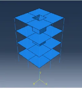
Problem 4: Steel Frame
This problem considers a small structure representing a bay of a larger building, with dimensions 7.3 m by 7.3 m (24 ft by 24 ft) in plan and 14.5 m (48 ft) high. It is a four-story steel frame, with concrete floor slabs and four interior shear walls, as shown in Figure 9. Note
actual structure. Beams and columns of the structure are modeled with frame elements and assigned W14X22 wide flange steel beam section properties. The floor slabs and shear walls were modeled as shell elements, with slab thickness of 300 mm (12 in). A bilinear stress-strain model for steel was used, with RVs taken as modulus of elasticity of steel, Es, with
mean of 200 GPa (29000 ksi) and COV of 0.1, and post-yield modulus of elasticity of steel,
Et, with mean of 8.3 GPa (1200 ksi) and COV of 0.1. Additional RVs are modulus of
elasticity of concrete, Ec, with mean of 24 GPa (3500 ksi) and COV of 0.1, and a uniform
pressure load P applied to the floor slabs, which was taken as the control variable, with mean of 3.35 or 4.31 kN/m2 (70 or 90 psf), depending on target reliability index considered, with COV of 0.1. The failure criterion is defined as the state where displacement at any point on the fourth floor slab exceeds 50 mm (2 in). The limit state function is given as:
g = 2 - D(Es,Et, Ec, P) (12)
All RVs were taken as normally distributed. The limit state function was evaluated using a commercial finite element analysis code (ABAQUS). Approximately 600 CPU hours were required for 1x10⁹ MCS samples to evaluate the exact solution. Two variants of this problem with higher complexity were also considered. In the first variant, resistance RVs were taken as partially correlated (ρ= 0.65) and COV of all resistance RVs was increased to 0.35. For the second variant, the number of resistance RVs was significantly increased to 52. In this problem, each of the 4 building floor slabs was divided into 4 sections as shown in Figure 9, and assigned a different modulus RV, as well as each of the 4 core shear walls for each floor, for 32 RVs Eci. The COV for each of these RVs was taken as 0.30, with ρ=0.30.
Additional RVs are 8 steel column elastic modulus RVs Esi andpost-yield modulus RVs Eti
(16 RVs total), where COV was taken as 0.3 and ρ=0.50, as well as a floor thickness RV ti for
Results for the more simple, 4 RV problems with uncorrelated RVs are shown in Table 7. As shown, it was found that all methods considered could provide reasonable solutions for the lower reliability case (P = 400 kN). However, for the higher reliability case (P = 312 kN), only the generalized lambda and Johnson distributions could provide solutions, with the Johnson distribution providing the lowest error at less than 4%. Considering the more complex problems in Table 8, it can be seen that in both cases (4 and 53 RV versions), only the Johnson distribution could produce a solution. Here, the more complex problems did not reduce the solution fidelity for the Johnson distribution, where error remains at 3-4%.
Conclusion and Recommendations
By coupling simple tools such as MCS, conditional expectation, and numerical integration and/or tail extrapolation, it was found that a wide variety of complex reliability problems can be consistently and accurately solved with reasonable computational effort using the modified conditional expectation approach implemented as failure sampling. Although no theoretical limitation exists to the types of problems that failure sampling can solve, the method has shown to be most useful for complex, computationally demanding reliability problems for which traditional methods may provide unacceptably inaccurate or unfeasibly computationally costly solutions, such as problems which have non-smooth limit state boundaries or that are otherwise highly nonlinear. In this study, an evaluation of alternative implementation methods was conducted. In particular, different approaches for estimating the PDF of the data sample, and the effect on the efficiency and accuracy of the solution were studied. In total, 85 limit state variations were investigated that covered a wide variety of problems, with parametric changes including the number of RVs, degree of non-linearity, and level of variance. In addition, several special limit state functions and two
evaluation were considered. From the investigation, it was found that increased accuracy can be obtained, for a wider variety of problems, with the Johnson distribution implementation rather than the generalized extreme value distribution or from the direct numerical integration or generalized lambda distribution approaches as originally suggested by Eamon and
Charmus (2011). In particular, unlike the three other methods considered, the Johnson distribution provided highly-accurate to reasonably-accurate solutions for every one of the problems evaluated in this study, even when greatly restricting computational effort.
In a small number of cases, other approaches provided superior results. These were a nonlinear, low reliability case and a case with a high number of normal RVs with high reliability, for which the generalized lambda distribution preformed best, as shown in example problem 1. In these cases, however, the advantage over the Johnson approach was relatively small. Therefore, if the failure sampling approach is considered for reliability analysis, the Johnson distribution implementation is generally recommended for use. If a potentially more refined selection procedure is desired, an appropriate goodness-of-fit test might be considered to estimate the expected effectiveness of a given approach for a
particular problem. An error metric such as that proposed by Eamon and Charumas (2011), which is based on differences between actual data and candidate curve CDF values, might serve this purpose, though its use requires additional effort. Given the wide applicability of the Johnson implementation, however, and the few cases for which alternative approaches were found to have a slight advantage, use of such a refinement does not appear to be particularly beneficial.
Acknowledgements
Funding was provided for this study by the National Science Foundation under Research Award No. 1127698, support for which is gratefully acknowledged.
Nomenclature
fQ PDF of Q
FR CDF of R(Xj)
fR PDF of R(Xj)
g(Xj) initial limit state function
g* failure sampling limit state function
pf failure probability
Q control random variable Q(u) GLD quantile function
R(Xi) random function within g* excluding Q
R R(Xi) represented as a single equivalent RV
u GLD PDF input parameter (probability) β reliability index
λi GLD parameter
Ф standard normal CDF
Γ transformation function for JSD γ,δ shape parameter for JSD
ξ location parameter for JSD λj scale parameter for JSD
k shape parameter for GEV μ location parameter for GEV σ scale parameter for GEV
References
Asif L, and Helmut M. (2000). "Estimating The Parameters Of The Generalized Lambda Distribution." ALGO Research Quarterly, Vol. 3, p. 47-58.
Au SK, and Beck JL. (2001). "Estimation Of Small Failure Probabilities In High Dimensions By Subset Simulation." Probabilistic Engineering Mechanics, Vol. 16, p. 263-277. Au SK, Ching J, and Beck JL. (2007). "Application Of Subset Simulation Methods To
Reliability Benchmark Problems." Structural Safety, Vol. 29, p. 183-193. Ayyub BM, and Chia CY. (1992). "Generalized Conditional Expectation For Structural
Reliability Assessment." Structural Safety, Vol. 11, p. 131-146.
Ayyub BM, and Haldar A. (1984). "Practical Structural Reliability Techniques." ASCE Journal of Structural Engineering, Vol. 110, p. 1707-1724.
Breitung K. (1984) "Asymptotic Approximations for Multinormal Integrals." ASCE Journal of Engineering Mechanics, Vol. 110, p. 357-366.
Cheng J, and Li QS. (2009). "Application Of Response Surface Methods To Solve Inverse Reliability Problems With Implicit Response Functions." Computational Mechanics, Vol. 43. p. 451-459.
Chiralaksanakul A, and Mahadevan S. (2005). "First Order Methods For Reliability Based Optimization." Journal of Mechanical Design, Vol. 127, p. 851-857.
Ditlevesen PG, and Bjerager P. (1988). "Plastic Reliability Analysis By Directional Simulation." ASCE Journal of Engineering Mechanics, Vol. 115, p. 1347-62.
Eamon C, and Charumas B. (2011). "Reliability Estimation Of Complex Numerical Problems Using Modified Conditional Expectation Method." Computers and Structures, Vol. 89, p. 181-188.
Reliability of Bridge Girders,” Journal of Bridge Engineering, Vol. 10, No. 2, p. 206-214.
Eamon C, Thompson M, and Liu Z. (2005). "Evaluation Of Accuracy And Efficiency Of Some Simulation And Sampling Methods In Structural Reliability Analysis." Structural Safety, Vol. 27, p. 356-392.
Engelund S, and Rackwitz R. (1993). "A Benchmark Study On Importance Sampling Techniques In Structural Reliability." Structural Safety, Vol. 12. p. 255-276. George F. (2007). "Johnsons System of Distribution and Microarray Data Analysis." PhD
Dissertation, Department of Mathematics, University of South Florida.
Gomes HM, and Awruch AM. (2004). "Comparison Of Response Surface And Neural Network With Other Methods For Structural Reliability Analysis." Structural Safety, Vol. 26, p. 49-67.
Haldar A, and Mahadevan S. (2000). "Probability, Reliability And Statistical Methods In Engineering Design." 1st ed. New York: John Wiley and Sons.
Iman RL, and Conover WJ. (1982). "A Distribution-Free Approach To Inducing Rank Correlation Among Input Variables". Communications in Statistics, Vol. 11. p. 311-334.
Karamchandani A, Bjerager P, and Cornell AC. (1989). "Adaptive Importance Sampling." Proceedings, International Conference on Structural Safety and Reliability
(ICOSSAR), San Francisco, CA., p. 855-862.
Karian ZA, and Dudewicz EJ. (2011). "Handbook Of Fitting Statistical Distributions With R." CRC Press.
Karian ZA, and Dudewicz EJ. (2003). “Comparison of GLD fitting methods: Superiority of percentile fits to moments in L2 norm.” Journal of the Iranian Statistical Society, Vol.
Melchers RE. (1999) "Structural Reliability Analysis and Prediction." 2nd ed. New York: John Wiley & Sons.
Ozaturk A, and Dale, RF. (1985). "Least Square Estimation Of The Parameters Of The Generalized Lambda Distribution." Technometrics, Vol. 27, p. 81-84.
Rackwitz R, and Fiessler B. (1978). "Structural Reliability Under Combined Random Load Sequences." Computers and Structures, Vol. 9, p. 484-494.
Rosowsky, D., Hassan, A., and Kumar, N. (1994). "Calibration of Current Factors in LRFD for Steel." Journal of Structural Engineering, Vol. 120, p. 2737-2746.
Rubinstein RY. (1981). "Simulation And The Monte Carlo Method." 1st ed. New York: John Wiley & Sons.
Slifker JF, and Shapiro SS. (1980). "The Johnson System: Selection And Parameter Estimation." Technometrics, Vol. 22, p. 239-246.
Szerszen, MM. and Nowak, AS. (2003). "Calibration of design code for buildings (ACI 318): Part 2 - Reliability analysis and resistance factors." ACI Structural Journal, Vo.-l. 100, No. 3, p. 383-391.
Wu YT. (1992). "An Adaptive Importance Sampling Method For Structural Systems Analysis, Reliability Technology." ASME Winter Annual Meeting, AD 28, p. 217-231.
List of Tables
Table 1. Random Variables for General Limit State Function Table 2. Parameter Values for General Limit State Function Table 3. Multiple Reliability Indices
Table 4. Maximum Function
Table 5. Displacement Limit State Function of Non-linear Static Truss Table 6. Stress Limit State Function of Non-linear Static Truss
Table 7. Steel Frame Structure
Table 8. Complex Steel Frame Structure
List of Figures
Figure 1. Example PDFs of g and R(xi) Figure 2. Effect of Linearity on Accuracy Figure 3. Effect of Linearity on Precision
Figure 4. Effect of Number of RVs on Accuracy Figure 5. Effect of Number of RVs on Precision Figure 6. Effect of Normality on Accuracy Figure 7. Effect of Normality on Precision Figure 8. Static Non-Linear Truss
Table 1. Random Variables for General Limit State Function Case n K RVs 2 RV linear 1 1 di, wj 5 RV linear 2 3 di, wDL1, wLLm* 15 RV linear 5 10 di, wDLm, wLLm* 2 RV nonlinear 1 1 di, Lj 5 RV nonlinear 1 1 di, wj, Lj, Ej, Ij 15 RV nonlinear 3 3 di, wj, Lj, Ej, Ij
Note: see eq. 7. i=1 to n and j=1 to k and indicate number of terms (RVs).
Table 2. Parameter Values for General Limit State Function Parameter* Value c 5/384 Lj 6.1 (m) Ej 2 x 10⁸ (kPa) Ij 6.452 x 10⁻⁴ (m4) wj 73600 (N/m) 𝑤𝐷𝐿 19300 (N/m) 𝑤𝐿𝐿 54300 (N/m)
Table 3. Multiple Reliability Indices
method no. of calls β %err Precision Exact solution 4.11 -- -- FORM -- Fail -- -- MCS 1000 N.F.* -- -- NI 1000 4.26 3.59 0.085 GLD 1000 Fail -- -- JSD 1000 3.93 4.33 0.101 GEV 1000 Fail -- -- * N.F. indicates no failures
Table 4. Maximum Function
method no. of calls β %err Precision Exact solution 3.53 -- -- FORM -- Fail -- -- MCS 1000 N.F.* -- -- NI 1000 3.66 3.66 0.035 GLD 1000 Fail -- -- JSD 1000 3.46 1.95 0.013 GEV 1000 Fail -- -- * N.F. indicates no failures
Table 5. Displacement Limit State Function of Non-linear Static Truss
nominal Actual % error mean P=267 mean P=223 Correlated method no. of calls no. of calls tolerance β %err β %err β %err Exact Solution 1×10⁹ 2.25 -- 3.59 -- 3.56 -- FORM 150 -- -- 1.96 12.9 3.12 13.1 Fail -- MCS 5000 5000 3% 2.54 11.4 N.F. -- N.F. -- NI 1000 5000 2.04 9.33 3.50 2.50 2.66 25.3 GLD 1000 5000 2.34 3.85 Fail -- Fail JSD 1000 5000 2.33 3.43 3.49 2.78 3.66 2.83 GEV 1000 5000 2.38 5.46 Fail -- Fail -- MCS 8000 8000 1% 2.32 3.02 N.F. -- NI 1000 8000 2.18 3.11 3.57 0.56 GLD 1000 8000 2.19 2.67 Fail -- JSD 1000 8000 2.28 1.05 3.61 0.41 GEV 1000 8000 2.34 3.85 Fail -- * N.F. indicates no failures
Table 6. Stress Limit State Function of Non-linear Static Truss
nominal Actual % error mean P=245 mean P=200 Correlated method no. of calls no. of calls tolerance β %err β %err β %err Exact Solution 1×10⁹ 1.78 -- 3.79 -- 3.63 -- FORM 250 -- -- Fail -- Fail -- Fail -- MCS 5000 5000 3% 1.87 4.81 N.F. -- N.F. -- NI 1000 5000 1.92 7.30 Fail -- 3.13 12.7 GLD 1000 5000 1.89 5.82 Fail -- Fail JSD 1000 5000 1.85 3.78 3.91 3.07 3.51 3.31 GEV 1000 5000 1.70 4.70 Fail -- Fail -- MCS 8000 8000 1% 1.77 0.56 N.F. -- NI 1000 8000 1.86 4.30 3.17 16.3 GLD 1000 8000 1.79 0.83 Fail -- JSD 1000 8000 1.75 1.46 3.82 0.78 GEV 1000 8000 1.73 2.76 Fail -- * N.F. indicates no failures
Table 7. Steel Frame Structure
nominal Actual mean P = 400 mean P = 312 method no. of calls no. of calls β %err β %err Exact Solution 1×10⁹ 1.803 -- 3.26 -- FORM 150 -- 1.86 3.27 Fail -- MCS 7000 7000 1.82 0.93 3.10 5.16 NI 1000 7000 1.84 2.01 Fail -- GLD 1000 7000 1.89 4.85 3.52 7.38 JSD 1000 7000 1.76 2.55 3.14 3.68 GEV 1000 7000 1.82 0.44 Fail --
Table 8. Complex Steel Frame Structure
nominal Actual 4 RVs 53 RVs method no. of calls no. of calls β %err β %err Exact Solution 1×10⁹ 3.68 -- 3.70 --
FORM 250 -- Fail -- Fail -- MCS 7000 7000 N.F. -- N.F. -- NI 1000 7000 Fail -- Fail -- GLD 1000 7000 Fail -- Fail -- JSD 1000 7000 3.52 4.37 3.59 3.06 GEV 1000 7000 Fail -- Fail --
(a)
(b)
(a) Calculating pf by sampling g directly results in a very small failure
region. (b) Failure region by sampling R(Xi).
Rmean 0.00 0.01 0.02 0.03 0.04 0.05 0.06 0.07 20 30 40 50 60 70 80 90 Pro b a b il ity d en sity f u n ctio n R(xi) MPP of g*
Failure region for R(xi)
g mean g = 0 0.00 0.01 0.02 0.03 0.04 0.05 0.06 0.07 -20 -10 0 10 20 30 40 50 P robabil it y densi ty fun ct ion g(xj) Failure region for
g(xj) (not visible)
(a)
Figure 1. Example PDFs of g and R(xi).
Figure 2. Effect of Linearity on Accuracy
0.0 0.1 0.2 0.3 0.4 0.5 0.6 0.7 0.8 0.9 1.0 1.1 NI GLD JSD GEV Me an ( C al cul at ed / E x act ) Method
Low Beta (Linear) High Beta (Linear) Low Beta (Non-Linear) High Beta (Non-linear)
Figure 3. Effect of Linearity on Precision 0.00 0.02 0.04 0.06 0.08 0.10 0.12 0.14 NI GLD JSD GEV P re ci si o n (C O V of Me an) Method
Low Beta (Linear) High Beta (Linear) Low Beta (Non-Linear) High Beta (Non-linear)
Figure 4. Effect of Number of RVs on Accuracy 0.0 0.1 0.2 0.3 0.4 0.5 0.6 0.7 0.8 0.9 1.0 1.1 NI GLD JSD GEV Me an (C al cul at ed / E x act ) Method
2 RV (Low Beta) 5 RV (Low Beta) 15 RV (Low Beta) 2 RV (High Beta) 5 RV (High Beta) 15 RV (High Beta)
Figure 5. Effect of Number of RVs on Precision 0.00 0.02 0.04 0.06 0.08 0.10 0.12 0.14 NI GLD JSD GEV P re ci si o n (C O V of Me an) Method
2 RV (Low Beta) 5 RV (Low Beta) 15 RV (Low Beta) 2 RV (High Beta) 5 RV (High Beta) 15 RV (High Beta)
Figure 6. Effect of Normality on Accuracy 0.0 0.1 0.2 0.3 0.4 0.5 0.6 0.7 0.8 0.9 1.0 1.1 NI GLD JSD GEV Me an (C al cul at ed / E x act ) Method
Normal (Low Beta) Non-normal (Low Beta) Normal (High Beta) Non-normal (High Beta)
Figure 7. Effect of Normality on Precision 0.00 0.02 0.04 0.06 0.08 0.10 0.12 0.14 NI GLD JSD GEV P re ci si o n (C O V of Me an) Method
Normal (Low Beta) Non-normal (Low Beta) Normal (High Beta) Non-normal (High Beta)
Figure 8. Static Non-Linear Truss
1 m 1 m
1 m