Simulation and Control of a Six Degree of Freedom Lower Limb
Exoskeleton
Mohammad Soleimani Amiria, Rizauddin Ramlia*, Mohd Aizat Ahmad Tarmizia, Mohd Faisal Ibrahimb
& Khashayar Danesh Narooei c
a Center for Materials Engineering and Smart Manufacturing, Faculty of Engineering and Built Environment, Universiti Kebangsaan Malaysia
b Center for Integrated Systems Engineering and Advanced Technologies, Faculty of Engineering and Built Environment, Universiti Kebangsaan Malaysia
cDepartment of Industrial Engineering, Faculty of Industry and Mining, Sistan and Baluchestan University, Zahedan, Iran
*Corresponding author: [email protected]
Received 08 October 2019, Received in revised form 12 February 2020 Accepted 30 March 2020, Available online 30 May 2020
ABSTRACT
In this paper, the development of controlling a six Degree of Freedom (DOF) Lower Limb Exoskeleton (LLE) model using the Robot Operating System (ROS) is presented. Moreover, this work proposes a method to analyze kinematic properties and control of the LLE before the prototype. The model of the LLE is described using Extensible Markup Language (XML) programming in the Unified Robot Description Format (URDF). The dynamic equation of the six-DoF LLE is determined by using Newton-Euler. In addition, a Proposition-Integral-Derivative (PID) controller is established in a feedback closed-loop control system. The PID controller is tuned via Ziegler-Nichols (Z-N). The tuned PID controller is tested in the Gazebo environment to confirm the performance of the proposed method. The nodes and topics flow chart of the programmed 3-D model of the LLE is described. Furthermore, a desired angular trajectory based on the phase on walking is defined for each joint of the LLE. The result shows that the actual pursue the desired angular trajectory for each joint. The average and maximum error of the angular trajectories for all the joints are less than 0.05 radian. It can be ascertained that our developed LLE model in the Gazebo simulator can be used for giving an overview of the walking pattern.
Keywords: Robot Operating System (ROS); 3-D simulation; Gazebo; Lower Limb Exoskeleton; Newton-Euler; rehabilitation robotics
INTRODUCTION
The exoskeleton is a wearable robot that increases the physical strength of the human muscle. For instance, in the case of rehabilitation, Lower Limb Exoskeleton (LLE) can assist patients who have lost the ability to move one part of their body, to recover to normal daily activities. Recently, many researchers from the field of the rehabilitation robot have paid attention in designing and controlling of an LLE because the number of patients who cannot walk due to injuries or getting old is increasing.
(Yali and Xingsong 2008) employed forward and inverse kinematics of their model to propose LLE. They verified the results of their work by using the combination of MATLAB- SIMULINK and ADAMS. Denavit-Hartengberg (D-H) method is a popular method to analyze inverse and forward kinematic. An analysis of forward and inverse D-H method has been used to obtain the torque to select electric-powered actuator for a six Degree of Freedom (DOF) LLE by (Shaari, Isa, and Jun 2015). In the other studies, inverse and forward kinematics using the D-H method and Lagrange equation of
LLE have been developed by(Baluch et al. 2012; Mohammadi Nasrabadi, Absalan, and Moosavian 2017; Xinyi et al. 2015). (Kim et al. 2013) designed mechanical hardware and sensor to determine the Center of Pressure (CoP) and position analysis for a 14 DOF LLE. They discussed an experiment to compare the actual and desired trajectory of the CoP. (Schemschat, Clever, and Mombaur 2017) represented an optimization-based simulation to determine the torque needed in the LLE. Furthermore, behaviors of walking of human with and without exoskeleton were compared to obtain information which is necessary for designing the LLE. (Song et al. 2017) worked on a Lower Extremity Power-assisted Exoskeleton (LEPEX) to increase human power for carrying heavy backpacks. They evaluated Lagrangian equations to select actuators for the LEPEX.
In some other researches in addition to the kinematics and dynamics equations, the control system of LLE has been developed. (Colombo and Morari 2004) worked on three algorithms for automated gait-pattern adoption, i.e. indirect dynamic, direct dynamic, and impedance control
base. These methods were tested on a healthy person and a patient to compare the performance of the algorithms. (Wu et al. 2016) studied an adaptive control for a 3-DOF LLE to recover the motion of the lower limb for stroke patients. Furthermore, an experiment with and without patients’ reaction has been carried out to observe the trajectory tracking error. (Huang and Ma 2017) worked on a combination of Respective Learning Control (RLC) and Neural Network (NN) regarding to human and external disturbance for knee and hip joints of an (Lin, Su, and Chen 2016) used an adaptive controller based on Fuzzy logic to reduce the effect of disturbance for a 2-DOF LLE. In another work, Genetic Algorithm (GA) is used to optimize the gain of NN for a 6-bar Stewart parallel robot used for rehabilitation purpose (Amini Azar, Akbarimajd, and Parvari 2016).
In recent years, researchers have shown a great interest in the Robot Operating System (ROS) as a tool of simulation and interfacing with sensors and actuators (Araújo et al. 2014; Maciel, Henriques, and Lages 2014). (Qian et al. 2014) employed ROS and Gazebo as a framework to simulate a 7-DOF manipulator. (Ergur and Ozkan 2014) proposed simulation of an industrial manipulator robot based on the ROS. They stated that saving time and eliminating the risk of damage for the robot are advantages of using ROS to develop trajectory planning methods for 3-D objects. (Beschi et al. 2015) represented the ROS as an educational tool of Proposition-Integral-Derivative PID controller for students. (Maciel et al. 2015) used ROS to simulate a simple model of a 6-DOF biped robot. They implemented a Multi-Input-Multi-Output (MIMO) non-linear controller based on the computed torque controller instead of a Single-Output-Single-Input (SISO) architecture that consists of PID controller, which is accomplished in ROS. (Kumar et al. 2017) considered a model consists of magnet Direct Current (DC) motors and an 8-bit microcontroller. This controller communicated with MATLAB via a serial/12c interface. In addition, they designed their model using SolidWorks and imported it to the MATLAB-Simulink. (Galli et al. 2017) used Robot System toolbox to connect MATLAB and ROS to minimize the trajectory error of a mobile robot.
In this paper, a new method of modelling an LLE has been developed in ROS and simulation of gait cycle movement in 3-dimensional (3-D) environment has been presented. In the next sections of this paper, after programming model using Extensible Markup Language (XML), the 3-D simulation of a 6-DOF LLE model in Gazebo and ROS platform is explained. The torque of each link is determined by using the Newton-Euler method. Finally, the angular trajectory of the joints of the LLE is considered as the results.
SIMULATION
ROS is a flexible framework and convenient to simulate and control hardware of a robot. In this paper, a model of an LLE, which is a 6-DOF manipulator consists of two femurs, two tibia, and two feet respectively has been studied. The kinematics and dynamics properties of the LLE are described in ROS using a package named Unified Robot Description Format (URDF).
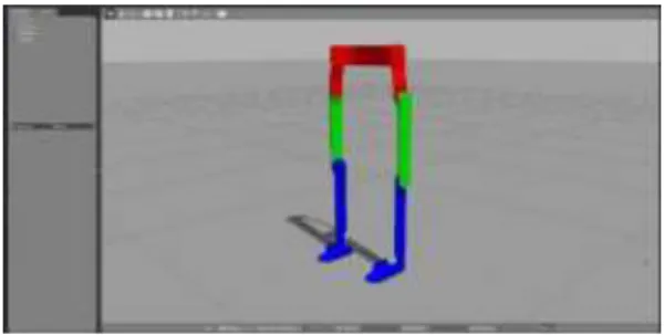
The LLE is modelled in the Gazebo, which is a 3-D open-source dynamic simulator with the capacity to simulate accurately and efficiently many variety types of robots in different indoor and outdoor environments. The Gazebo offers physics simulation at a much higher degree of fidelity, a suite of sensors, and interfaces for both users and programs. ROS-control packages and the Gazebo plugin adapter can be fulfilled to simulate a robot's controllers. The ability to implement and run robot controllers with an eye to both real-time performance and sharing of controllers is provided by the ROS-control framework. ROS-control is a package that includes controller interfaces, controller managers, transmissions and hardware-interfaces (Chitta et al. 2017). Moreover, the Ros-control package takes information directly from the robot's actuator's encoders and a desired input set point. In other words, it is a generic control loop feedback mechanism that uses normally a PID controller (Azar and Vaidyanathan 2015). Figure 1 shows the model of the LLE in Gazebo.
FIGURE 1. The model of the LLE in Gazebo The Gazebo uses the Open Dynamics Engine (ODE) to determine the dynamics and kinematics connected with articulated rigid bodies. The ODE is an open-source physic engine simulating rigid body dynamics. Several features such as numerous joints, collision detection, mass and rotational functions containing arbitrary triangle meshes are provided in ODE (Koenig and Howard 2004). This dynamic simulator solves the Newton-Euler equation, which is derived from Newton’s second law (Drumwright et al. 2010).
DYNAMIC MODEL
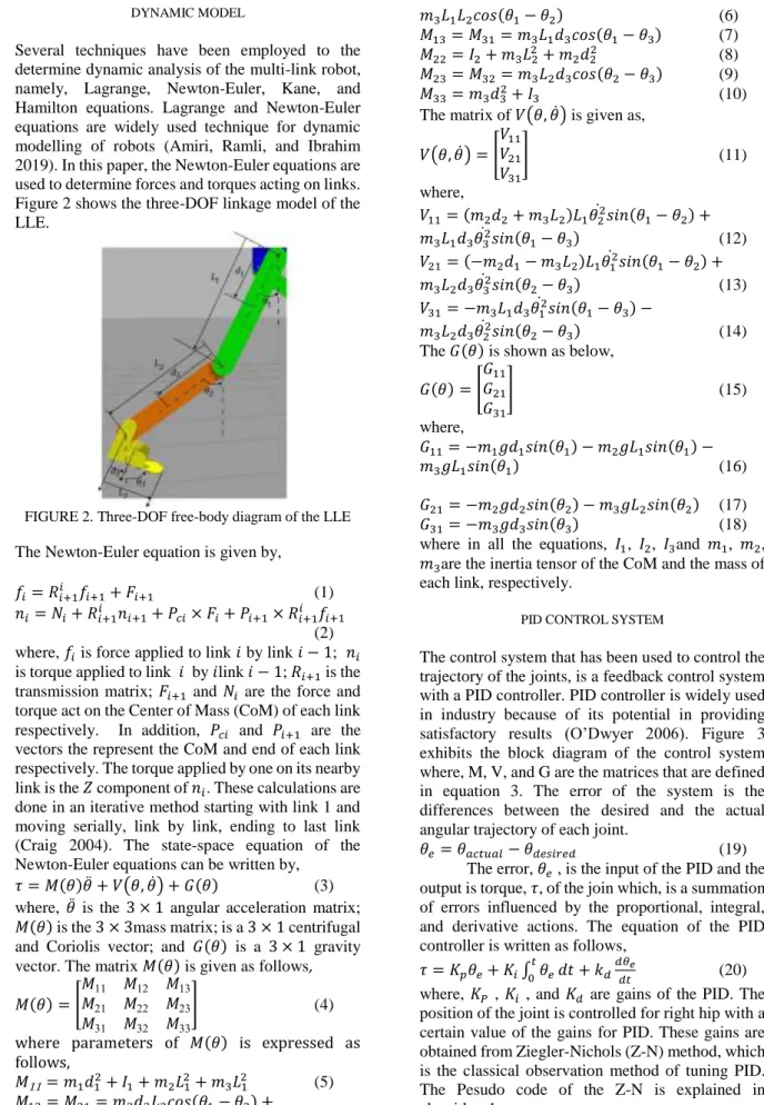
Several techniques have been employed to the determine dynamic analysis of the multi-link robot, namely, Lagrange, Newton-Euler, Kane, and Hamilton equations. Lagrange and Newton-Euler equations are widely used technique for dynamic modelling of robots (Amiri, Ramli, and Ibrahim 2019). In this paper, the Newton-Euler equations are used to determine forces and torques acting on links. Figure 2 shows the three-DOF linkage model of the LLE.
FIGURE 2. Three-DOF free-body diagram of the LLE The Newton-Euler equation is given by,
𝑓𝑖= 𝑅𝑖+1𝑖 𝑓𝑖+1+ 𝐹𝑖+1 (1) 𝑛𝑖= 𝑁𝑖+ 𝑅𝑖+1𝑖 𝑛𝑖+1+ 𝑃𝑐𝑖× 𝐹𝑖+ 𝑃𝑖+1× 𝑅𝑖+1𝑖 𝑓𝑖+1
(2) where, 𝑓𝑖 is force applied to link 𝑖 by link 𝑖 − 1; 𝑛𝑖 is torque applied to link 𝑖 by 𝑖link 𝑖 − 1; 𝑅𝑖+1 is the transmission matrix; 𝐹𝑖+1 and 𝑁𝑖 are the force and torque act on the Center of Mass (CoM) of each link respectively. In addition, 𝑃𝑐𝑖 and 𝑃𝑖+1 are the vectors the represent the CoM and end of each link respectively. The torque applied by one on its nearby link is the 𝑍 component of 𝑛𝑖. These calculations are done in an iterative method starting with link 1 and moving serially, link by link, ending to last link (Craig 2004). The state-space equation of the Newton-Euler equations can be written by,
𝜏 = 𝑀(𝜃)𝜃¨ + 𝑉(𝜃, 𝜃˙) + 𝐺(𝜃) (3) where, 𝜃¨ is the 3 × 1 angular acceleration matrix; 𝑀(𝜃) is the 3 × 3mass matrix; is a 3 × 1 centrifugal and Coriolis vector; and 𝐺(𝜃) is a 3 × 1 gravity vector. The matrix 𝑀(𝜃) is given as follows, 𝑀(𝜃) = [
𝑀11 𝑀12 𝑀13
𝑀21 𝑀22 𝑀23
𝑀31 𝑀32 𝑀33
] (4)
where parameters of 𝑀(𝜃) is expressed as follows, 𝑀11= 𝑚1𝑑12+ 𝐼1+ 𝑚2𝐿12+ 𝑚3𝐿21 (5) 𝑀12= 𝑀21= 𝑚2𝑑2𝐿2𝑐𝑜𝑠(𝜃1− 𝜃2) + 𝑚3𝐿1𝐿2𝑐𝑜𝑠(𝜃1− 𝜃2) (6) 𝑀13= 𝑀31= 𝑚3𝐿1𝑑3𝑐𝑜𝑠(𝜃1− 𝜃3) (7) 𝑀22= 𝐼2+ 𝑚3𝐿22+ 𝑚2𝑑22 (8) 𝑀23= 𝑀32= 𝑚3𝐿2𝑑3𝑐𝑜𝑠(𝜃2− 𝜃3) (9) 𝑀33= 𝑚3𝑑32+ 𝐼3 (10)
The matrix of 𝑉(𝜃, 𝜃˙) is given as, 𝑉(𝜃, 𝜃˙) = [𝑉𝑉1121 𝑉31 ] (11) where, 𝑉11= (𝑚2𝑑2+ 𝑚3𝐿2)𝐿1𝜃˙ 𝑠𝑖𝑛(𝜃122 − 𝜃2) + 𝑚3𝐿1𝑑3𝜃˙ 𝑠𝑖𝑛(𝜃132 − 𝜃3) (12) 𝑉21= (−𝑚2𝑑1− 𝑚3𝐿2)𝐿1𝜃˙ 𝑠𝑖𝑛(𝜃12 1− 𝜃2) + 𝑚3𝐿2𝑑3𝜃˙ 𝑠𝑖𝑛(𝜃32 2− 𝜃3) (13) 𝑉31= −𝑚3𝐿1𝑑3𝜃˙ 𝑠𝑖𝑛(𝜃12 1− 𝜃3) − 𝑚3𝐿2𝑑3𝜃˙ 𝑠𝑖𝑛(𝜃222 − 𝜃3) (14) The 𝐺(𝜃) is shown as below,
𝐺(𝜃) = [ 𝐺11 𝐺21 𝐺31] (15) where, 𝐺11= −𝑚1𝑔𝑑1𝑠𝑖𝑛(𝜃1) − 𝑚2𝑔𝐿1𝑠𝑖𝑛(𝜃1) − 𝑚3𝑔𝐿1𝑠𝑖𝑛(𝜃1) (16) 𝐺21= −𝑚2𝑔𝑑2𝑠𝑖𝑛(𝜃2) − 𝑚3𝑔𝐿2𝑠𝑖𝑛(𝜃2) (17) 𝐺31= −𝑚3𝑔𝑑3𝑠𝑖𝑛(𝜃3) (18) where in all the equations, 𝐼1, 𝐼2, 𝐼3and 𝑚1, 𝑚2, 𝑚3are the inertia tensor of the CoM and the mass of each link, respectively.
PID CONTROL SYSTEM
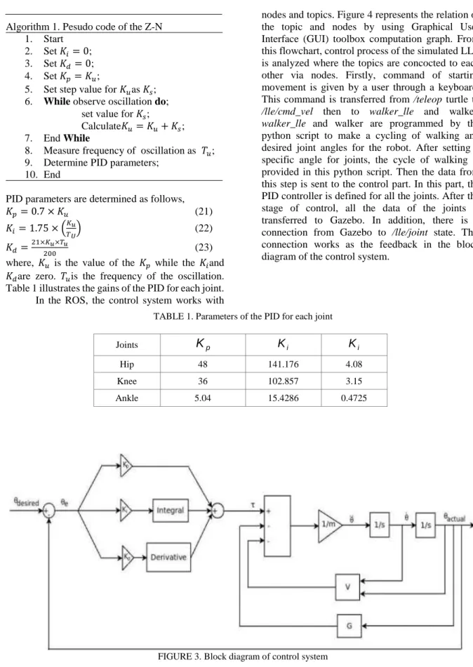
The control system that has been used to control the trajectory of the joints, is a feedback control system with a PID controller. PID controller is widely used in industry because of its potential in providing satisfactory results (O’Dwyer 2006). Figure 3 exhibits the block diagram of the control system where, M, V, and G are the matrices that are defined in equation 3. The error of the system is the differences between the desired and the actual angular trajectory of each joint.
𝜃𝑒= 𝜃𝑎𝑐𝑡𝑢𝑎𝑙− 𝜃𝑑𝑒𝑠𝑖𝑟𝑒𝑑 (19) The error, 𝜃𝑒 , is the input of the PID and the output is torque, 𝜏, of the join which, is a summation of errors influenced by the proportional, integral, and derivative actions. The equation of the PID controller is written as follows,
𝜏 = 𝐾𝑝𝜃𝑒+ 𝐾𝑖∫ 𝜃𝑒0𝑡 𝑑𝑡 + 𝑘𝑑𝑑𝜃𝑑𝑡𝑒 (20) where, 𝐾𝑃 , 𝐾𝑖 , and 𝐾𝑑 are gains of the PID. The position of the joint is controlled for right hip with a certain value of the gains for PID. These gains are obtained from Ziegler-Nichols (Z-N) method, which is the classical observation method of tuning PID. The Pesudo code of the Z-N is explained in algorithm 1.
Algorithm 1. Pesudo code of the Z-N 1. Start
2. Set 𝐾𝑖= 0; 3. Set 𝐾𝑑= 0; 4. Set 𝐾𝑝= 𝐾𝑢;
5. Set step value for 𝐾𝑢as 𝐾𝑠; 6. While observe oscillation do;
set value for 𝐾𝑠; Calculate𝐾𝑢= 𝐾𝑢+ 𝐾𝑠; 7. End While
8. Measure frequency of oscillation as 𝑇𝑢; 9. Determine PID parameters;
10. End
PID parameters are determined as follows,
𝐾𝑝= 0.7 × 𝐾𝑢 (21)
𝐾𝑖= 1.75 × (𝐾𝑢
𝑇𝑈) (22)
𝐾𝑑=21×𝐾200𝑢×𝑇𝑢 (23)
where, 𝐾𝑢 is the value of the 𝐾𝑝 while the 𝐾𝑖and 𝐾𝑑are zero. 𝑇𝑢is the frequency of the oscillation. Table 1 illustrates the gains of the PID for each joint. In the ROS, the control system works with
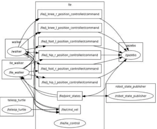
nodes and topics. Figure 4 represents the relation of the topic and nodes by using Graphical User Interface (GUI) toolbox computation graph. From this flowchart, control process of the simulated LLE is analyzed where the topics are concocted to each other via nodes. Firstly, command of starting movement is given by a user through a keyboard. This command is transferred from /teleop turtle to
/lle/cmd_vel then to walker_lle and walker.
walker_lle and walker are programmed by the python script to make a cycling of walking and desired joint angles for the robot. After setting a specific angle for joints, the cycle of walking is provided in this python script. Then the data from this step is sent to the control part. In this part, the PID controller is defined for all the joints. After the stage of control, all the data of the joints is transferred to Gazebo. In addition, there is a connection from Gazebo to /lle/joint state. This connection works as the feedback in the block diagram of the control system.
TABLE 1. Parameters of the PID for each joint
Joints
Hip 48 141.176 4.08
Knee 36 102.857 3.15
Ankle 5.04 15.4286 0.4725
FIGURE 3. Block diagram of control system
FIGURE 4. Flow chart of nodes and topics
RESULTS AND DISCUSSION
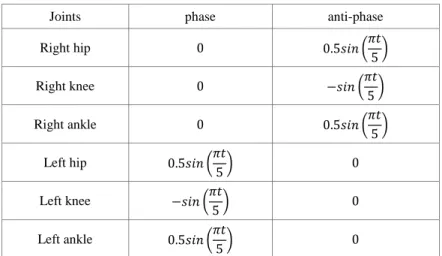
Desired angles of joints and the regulation of their movement have been used as input into the system. The desired pattern of walking for all joints is divided into two parts, which are phase and anti-phase. The cycle of walking starts from phase condition. Table 2 shows the phase and anti-phase condition for each joint of right and left side of the LLE. For instance, the value of the angular trajectory for the joints of the right leg is zero and in the anti-phase condition, while the angular trajectory is a sine function for the joints of the left leg. On other words, each gait cycle is divided into two phases, which are stance phase and swing phase. During stance phase, the foot remains in touch with the ground, and in the swing phase, the foot is not in touch with the ground. When one leg is in swing phase, the other leg is in stance phase. Therefore, zero represents the stance phase and sine function shows that the leg is in swing phase. Furthermore, the absolute formulations of hip and ankle are same
in each phase. However, the absolute value of the angular trajectory for left and right knees is twice more than this value for hip and ankle because based on the standard gait cycle the maximum angular knee position is almost two times than hip.
Figure 5 illustrates the angular trajectory of hip, knee and ankle joints for both left and right legs respectively. The steady and non-fluctuating movement of the joints shows that the control system is working properly. The result shows the actual follows the desired angular trajectory in each joint. The gait cycle of the LLE last two seconds. At the first second of one gait cycle, when the left leg is doing the swing phase, the right leg is in the stance phase. Constantly, in the second half of one gait cycle, while the left leg is the in the stance phase, the right side’s joints are doing their swing phase. Table3 represents the average and maximum error of the angular trajectories for all the joints, in which AE is the average error and ME is the maximum error.
As can be seen in the table3 the average error and maximum are less than 0.05 radian which is in the acceptable zone based on (Wu et al. 2016).
TABLE 2. The equation of desired angular trajectory for each joint
Joints phase anti-phase
Right hip 0 0.5𝑠𝑖𝑛(𝜋𝑡 5) Right knee 0 −𝑠𝑖𝑛(𝜋𝑡 5) Right ankle 0 0.5𝑠𝑖𝑛(𝜋𝑡 5) Left hip 0.5𝑠𝑖𝑛(𝜋𝑡 5) 0 Left knee −𝑠𝑖𝑛(𝜋𝑡 5) 0 Left ankle 0.5𝑠𝑖𝑛(𝜋𝑡 5) 0
TABLE 3. Angular trajectory error for the joints
Left hip Right hip Left knee Right knee Left ankle Right ankle
AE 0.0031 0.0029 0.0027 0.0035 0.0009 0.0009
ME 0.0092 0.0089 0.009 0.012 0.0032 0.0031
(a) Left hip (b) Right hip
(e) Left ankle (f) Right ankle FIGURE 5. Angular trajectory of the joints
CONCLUSION
In this study, the trajectory planning and control of the model of a 6-DOF LLE were presented. The LLE consists of three DOF for each leg, which are one DOF for each hip, knee and ankle respectively. The model of the LLE was defined by XML script an implemented in Gazebo environment. Moreover, the PID controller was developed for each joint. The desired trajectory was defined for the model of the LLE in Gazebo. Additionally, the Newton-Euler equations were solved by ODE to measure forces and torques of each link.
The walking cycle of the LLE in Gazebo consisted of stance and swing phase. The stance phase for each joint was a zero function while the swing phase was a sine function. The results showed that the actual followed the desired angular trajectory for each joint. Furthermore, the Gazebo stimulation is useful to visualize the motion of the LLE before the prototype. In conclusion, it can be proven that our new LLE model simulated in Gazebo is suitable to create a device for walk training.
ACKNOWLEDGMENT
The authors would like to thank Universiti Kebangsaan Malaysia (UKM) and the Ministry of Education Malaysia for financial support received
under research grant ERGS
/1/2012/TK01/UKM/02/2. REFERENCES
Amini Azar, Wahab, Adel Akbarimajd, and Esmaeil Parvari. 2016. Intelligent Control Method of a 6-DOF Parallel Robot Used for Rehabilitation Treatment in Lower Limbs.
Automatika ‒ Journal for Control, Measurement, Electronics, Computing and Communications 57(2):466–76.
Amiri, Mohammad Soleimani, Rizauddin Ramli, and Mohd Faisal Ibrahim. 2019. Hybrid Design of PID Controller for Four DoF Lower Limb Exoskeleton. Applied Mathematical Modelling 72:17–27.
Araújo, André, David Portugal, Micael S. Couceiro, and Rui P. Rocha. 2014. Integrating Arduino-Based Educational Mobile Robots in ROS.
Journal of Intelligent and Robotic Systems: Theory and Applications 77(2):281–98. Azar, Ahmad Taher and Sundarapandian
Vaidyanathan. 2015. Computational Intelligence Applications in Modeling and Control. Springer.
Baluch, Tawakal Hasnain, Adnan Masood, Javaid Iqbal, Umer Izhar, and Umar Shahbaz Khan. 2012. Kinematic and Dynamic Analysis of a Lower Limb Exoskeleton. International Journal of Mechanical, Aerospace, Industrial, Mechatronic and Manufacturing Engineering, 6(9):812–26.
Beschi, Manuel, Riccardo Adamini, Alberto Marini, and Antonio Visioli. 2015. Using of the Robotic Operating System for PID Control Education. IFAC-Papers Online, 48(29):87– 92.
Chitta, Sachin, Eitan Marder-Eppstein, Wim Meeussen, Vijay Pradeep, Adolfo Rodríguez Tsouroukdissian, Jonathan Bohren, David Coleman, Bence Magyar, Gennaro Raiola, Mathias Lüdtke, and Enrique Fernandez Perdomo. 2017. Ros_control: A Generic and Simple Control Framework for ROS. The Journal of Open Source Software, 2(20):456. Colombo, G. and M. Morari. 2004. Rehabilitation With a 4-DOF Robotic Orthosis. IEEE Transactions on Robotics, 20(3):574–82. Craig, John J. 2004. “Introduction to Robotics:
Mechanics and Control 3rd.” Prentice Hall 1(3):408.
Drumwright, Evan, John Hsu, Nathan Koenig, and Dylan Shell. 2010. “Extending Open Dynamics Engine for Robotics Simulation.”
Lecture Notes in Computer Science (Including Subseries Lecture Notes in Artificial Intelligence and Lecture Notes in Bioinformatics) 6472 LNAI:38–50.
Ergur, Serkan and Metin Ozkan. 2014. Trajectory Planning of Industrial Robots for 3-D Visualization. IEEE International Symposium on Robotics and Manufacturing Automation Trajectory, 206–11.
Galli, M., R. Barber, S. Garrido, and L. Moreno. 2017. Path Planning Using Matlab-ROS Integration Applied to Mobile Robots. IEEE International Conference on Autonomous Robot Systems and Competitions, ICARSC,
98–103.
Huang, Deqing and Lei Ma. 2017. Neural Network Control of Lower Limb Rehabilitation Exoskeleton with Repetitive Motion.
Proceedings of the 36th Chinese Control Conference, 3403–8.
Kim, Jung Hoon, Jeong Woo Han, Deog Young Kim, and Yoon Su Baek. 2013. Design of a Walking Assistance Lower Limb Exoskeleton for Paraplegic Patients and Hardware Validation Using CoP.
International Journal of Advanced Robotic Systems, 10(2).
Koenig, N. and A. Howard. 2004. “Design and Use Paradigms for Gazebo, an Open-Source Multi-Robot Simulator. IEEE/RSJ International Conference on Intelligent Robots and Systems (IROS), 3:2149–54. Kumar, Akshay, Anshul Mittal, Rajat Arya, Akash
Shah, Sharad Garg, and Rajesh Kumar. 2017. Animation of Working Model. International Conference on Inventive Systems and Control, 1–5.
Lin, Chih-wei, Shun-feng Su, and Ming-chang Chen. 2016. Indirect Adaptive Fuzzy Decoupling Control with a Lower Limb Exoskeleton. Proceedings of 2016 International Conference on Advanced Robotics and Intelligent Systems, 1-5. Maciel, Eduardo Henrique, Renato Ventura Bayan
Henriques, and Walter Fetter Lages. 2014. Control of a Biped Robot Using the Robot Operating System. Joint Conference on Robotics: SBR-LARS Robotics Symposium and Robocontrol, 247–52.
Maciel, Eduardo Henrique, Renato Ventura, Bayan Henriques, and Walter Fetter Lages. 2015. Development and Control of the Lower Limbs of a Biped Robot. Communications in Computer and Information Science,
507:133–52.
Mohammadi Nasrabadi, Ali A., Farshid Absalan, and S. Ali A. Moosavian. 2017. Design, Kinematics and Dynamics Modeling of a Lower-Limb Walking Assistant Robot. 4th
RSI International Conference on Robotics and Mechatronics, 319–24.
O’Dwyer, Aidan. 2006. PI and PID Controller Tuning Rules: An Overview and Personal Perspective. Proceedings of the IET Irish Signals and Systems Conference, 161–66. Qian, Wei, Zeyang Xia, Jing Xiong, Yangzhou Gan,
Yangchao Guo, Shaokui Weng, Hao Deng, Ying Hu, and Jianwei Zhang. 2014. Manipulation Task Simulation Using ROS and Gazebo. IEEE International Conference on Robotics and Biomimetics, IEEE ROBIO,
2594–98.
Schemschat, R. Malin, Debora Clever, and Katja Mombaur. 2017. Optimization Based Analysis of Push Recovery during Walking Motions to Support the Design of Lower-Limb Exoskeletons. IEEE International Conference on Simulation, Modeling, and Programming for Autonomous Robots,
SIMPAR, 31(22):224–31.
Shaari, N. A., Ida S. Isa, and Tan Chee Jun. 2015. Torque Analysis of The Lower Limb Exoskeleton Robot Design by Using Solidwork Software. ARPN Journal of Engineering and Applied Sciences, 10(19):1– 10.
Song, Shengli, Xinglong Zhang, Qing Li, Husheng Fang, Qing Ye, and Zhitao Tan. 2017. Dynamic Analysis and Design of Lower Extremity Power-Assisted Exoskeleton.
Wearable Sensors and Robots, 399.
Wu, Junpeng, Jinwu Gao, Rong Song, Rihui Li, Yaning Li, and Lelun Jiang. 2016. The Design and Control of a 3DOF Lower Limb Rehabilitation Robot. Mechatronics, 33:13– 22.
Xinyi, Zhang, Wang Haoping, Tian Yang, Wang Zefeng, and Peyrodie Laurent. 2015. “Modeling, Simulation &Amp; Control of Human Lower Extremity Exoskeleton.” 2015 34th Chinese Control Conference (CCC) (4):6066–71.
Yali, Han and Wang Xingsong. Kinematics Analysis of Lower Extremity Exoskeleton. 2008
Chinese Control and Decision Conference,