Analytical energy gradient for reference interaction site model self-consistent field explicitly including spatial electron density distribution

Title

Analytical energy gradient for reference interaction site model

self-consistent field explicitly including spatial electron density

distribution

Author(s)

Yokogawa, Daisuke; Sato, Hirofumi; Sakaki, Shigeyoshi

Citation

The Journal of Chemical Physics (2009), 131(21)

Issue Date

2009-12-03

URL

http://hdl.handle.net/2433/123546

Right

Copyright 2009 American Institute of Physics. This article may

be downloaded for personal use only. Any other use requires

prior permission of the author and the American Institute of

Physics. The following article appeared in The Journal of

Chemical Physics 131, 214504 (2009) and may be found at

http://link.aip.org/link/JCPSA6/v131/i21/p214504/s1

Type

Journal Article

Textversion

publisher

Analytical energy gradient for reference interaction site model

self-consistent field explicitly including spatial electron density distribution

Daisuke Yokogawa, Hirofumi Sato,a兲 and Shigeyoshi Sakaki

Department of Molecular Engineering, Graduate School of Engineering, Kyoto University, Nishikyo-ku, Kyoto 615-8510, Japan

共Received 18 August 2009; accepted 29 October 2009; published online 3 December 2009兲 Analytical energy gradient formula was derived for reference interaction site model self-consistent field explicitly including spatial electron density distribution 共RISM-SCF-SEDD兲. RISM-SCF-SEDD is a combination method ofab initio electronic structure theory and statistical mechanics for molecular liquids 关D. Yokogawa et al., J. Chem. Phys. 126, 244504 共2007兲兴. As shown previously, RISM-SCF-SEDD is numerically stable and has expanded the applicability of the solvation theory. The energy gradient is an indispensable tool to compute molecular geometry and its implementation further extends the capability of RISM-SCF-SEDD. The present method was applied to chemical systems in aqueous solution; hydration structure and geometry of phosphate anion PO₄3−and tautomerization between 2-pyridone and 2-hydroxypyridine. Compared to available experimental data, the present method correctly reproduced the geometries and relative energies of solvated molecules with microscopic solvent distribution. It is clearly shown that highly sophisticated quantum chemical calculation such as coupled cluster with single and double and perturbative triple excitations coupled with solvation effect is a powerful tool to accurately evaluate molecular properties. ©2009 American Institute of Physics.

关doi:10.1063/1.3265856兴

I. INTRODUCTION

Molecular geometry is a fundamental information to un-derstand chemical phenomena and extensive studies are per-formed over a long period of time. For molecule in isolated state, several methods become mature and precise determi-nation of geometrical parameters is realizable, especially for small polyatomic molecule. Ab initio electronic structure computation is now routinely available due to the develop-ment of energy gradient technique for various electronic structure theories and highly accurate geometrical parameters—the error is sometimes smaller than experimen-tal one—are available. Contrastingly, the situation is differ-ent for molecule in solution phase. Most widely employed experimental approaches to obtain geometrical data are x-ray and neutron scatterings, which allow us to estimate bond lengths and bond angles of solvated molecule. However, in general, it is still experimentally difficult to obtain geometri-cal parameters in high accuracy.

Nowadays, development ofab initioquantum chemical methods involving solvation effect has been strenuously pro-ceeding. Polarizable continuum model1共PCM兲is one of the most popular methods, in which solvent is treated as dielec-tric continuum surrounding the solute molecule.2The energy gradient technique has been developed in 1994共Ref.2兲and now it is routinely executable in various program packages. The method is very useful but it has been well recognized that the evaluation of hydrogen bonding is rather poor.3 To make up for the defect, a few solvent molecules are often considered explicitly within the system. Quantum

mechani-cal and molecular mechanics 共QM/MM兲 method utilizing molecular simulation method such as molecular dynamics naturally takes into account the effect of microsolvation. In this method, solute molecule is computed with quantum chemical calculation under the potential produced by the sur-rounding solvent molecules that are dealt with classical me-chanics. Statistically averaged energy gradient is applied to obtain equilibrium geometry in solution.4,5 In principle, ac-curate geometrical parameters are expected to be obtained if adequate ensemble of solvent configuration is feasible.

Reference interaction site model self-consistent field

共RISM-SCF兲 is another method,6–8 where solvent is treated with statistical mechanics and the electronic structure is evaluated under the electric fields generated by microscopic solvation structure, i.e., distribution function. Thanks to the analytic, algebraic nature of RISM theory, statistical en-semble of solvent configuration is perfectly computed with reasonable cost. The analytical energy gradient formula has been proposed in the early stage,8and successfully applied to a large number of systems.9,10 However, the calculation of the original RISM-SCF often diverges when the system con-tains buried atoms. Recently, we proposed a new generation of RISM-SCF to overcome the weak point.11 In the new method, spatial electron density distribution共SEDD兲was ex-plicitly introduced in RISM-SCF scheme 共 RISM-SCF-SEDD兲. Not only the description of physical nature of chemical system becomes accurate but also the numerical stability of the computation is significantly improved. In this article, we derived an analytical gradient formula based on RISM-SCF-SEDD. To obtain accurate geometry in solution phase, the RISM-SCF-SEDD calculation was performed

a兲_{Electronic mail: [email protected].}

with density functional theory 共DFT兲 and coupled cluster expansion using single and double excitations with perturba-tion treatment of triples关CCSD共T兲兴.

This article is organized as follows. In Sec. II, the equa-tions employed in this work were derived. The detail of the calculation was described in Sec. III. The present method was applied to two demonstrative examples; hydration struc-ture and geometry of phosphate anion PO₄3−in aqueous phase and the tautomerization between 2-pyridone 共PY兲 and 2-hydroxypyridine 共HP兲in aqueous phase. The results were compared with available experimental data in Sec. IV.

II. THEORY

Before deriving the equation of energy gradient, we briefly summarize key equations employed in this work. Sol-vation structure around a solute molecule is calculated by RISM equation with hypernetted-chain共HNC兲closure,

h_␣s UV =

兺

␥t ␻␣␥U

*

c␥t UV

*

␹ts VV , 共1兲 ␹ts VV =␻ts V +␳t V hts VV , 共2兲 h_␣s UV = exp关−␤␾_␣s UV +h_␣s UV −c_␣s UV_兴 − 1, 共3兲

where␤= 1/kBTandkBis Boltzmann’s constant.h_␣s UV

andc_␣UV_s are total and direct correlation functions between solute共U兲 site ␣ and solvent 共V兲 site s, h_stVV is the total correlation function for solvent, and兵␾_␣UV_s其is the solute-solvent interac-tion potential. 兵␻_␣␥U其and兵␻_stV其are intramolecular correlation functions, which define solute and solvent molecular geom-etries, respectively. ␳_tV is the number density of the solvent sitet.

The solute-solvent interaction potential, 兵␾_␣s UV_其

, is the sum of Coulombic and Lennard-Jones共LJ兲terms,

␾␣s UV_共 r兲=␾_␣s CL_共 r兲+ 4⑀_␣s

再

冉

␴␣s r

冊

12 −

冉

␴␣s r

冊

6

冎

. 共4兲 The Coulombic term ␾_␣s

CL_共

r兲 is usually written as classical expression, namely,q_␣qs/r. However, in RISM-SCF-SEDD,

it is calculated directly from electron density ␳e共r兲 of the

solute molecule.11␳e共r兲is expanded with the spherical

aux-iliary basis sets共ABSs兲,兵fi其, on each solute atomic site, ␳e共r兲=

兺

i

difi共r兲, 共5兲

with the coefficient dand ABS,␾_␣CL_s共r兲 is thus expressed as follows: ␾␣s CL_共 r兲= −qs

兺

i苸␣ di

冕

fi共r

⬘

兲 兩r−r

⬘

兩dr

⬘

+ qsZ␣ r , 共6兲

where qs is a partial charge on a solvent site s, Z␣ is the

nuclear charge of a solute atomic site␣, andR_␣ is the posi-tion vector of atomic site␣. The expansion coefficient兵di其is

evaluated by the following equation:

d=X−1tr共PY兲−Z

t

X−1tr共PY兲−Ne ZtX−1Z X

−1_{Z, 共7兲}

where P is usual “P-matrix” related to the electron density andNeis the number of electron in solute molecule.X, Y,

andZ are matrices which are defined with the given ABSs, atomic orbitals, and geometry of solute molecule, as follows:11

Xij=

冕冕

fi共r1兲兩r1−r2兩fj共r2兲dr1dr2, 共8兲

Y_␮␯,i=

冕冕

␹␮共r1兲␹␯共r1兲兩r1−r2兩fi共r2兲dr1dr2, 共9兲

Zi=

冕

fi共r兲dr, 共10兲

where␹is the basis function employed in molecular orbital calculation.

In the RISM-HNC framework, excess chemical potential

共⌬␮兲given by ⌬␮= −1 ␤

兺

␣s ␳s V

冕

dr

冋

c_␣s UV_共 r兲− 1 2共h␣s UV_共 r兲兲2+ 1 2h␣s UV_共 r兲c_␣s UV_共 r兲

册

= −1 ␤

兺

␣s ␳s V

冕

dr

冋

e−␤␾␣s UV 共r_兲+t_␣UV_s共r_兲 − 1 −t_␣s UV_共 r兲 + 1 2共h␣s UV_共 r兲兲2−h_␣s UV_共 r兲t_␣s UV_共 r兲

册

+ 1 共2␲兲3␤

冕

dk

冋

兺

_␣s ␳s V hˆ_␣s UV_共 k兲cˆ_␣s UV_共 k兲 − 1 2_␣␥

兺

st ␳s V cˆ_␣s UV cˆ_␥t UV_␹ ˆst VV_␻ ˆ_␣␥U

册

, 共11兲 wheret_␣s UV =h_␣s UV −c_␣s UV

and hat共ˆ兲means the function in recip-rocal space. RISM equation and HNC closure are derived from Eq.共11兲by the well-known variational stationarity.12In analogy with the RISM-HNC as well as with the original RISM-SCF method,8Acorresponding to the Helmholtz free energy of the system is defined as follows:

A=E_solute+⌬␮, where E_solute=具⌿兩H兩⌿典. 共12兲 H is the Hamiltonian for a solute molecule in the standard quantum chemical method and⌿is the wave function of the solute molecule in solvent. Thanks to the variational station-arity of RISM-HNC theory, the first derivative of A with respect to the nuclear coordinate of the solute moleculeRais

simply given by共see Appendix for the detail兲

⳵A ⳵Ra =⳵Esolute ⳵Ra +⳵⌬␮ ⳵Ra =⳵Esolute ⳵Ra −Vt⳵d ⳵Ra − 1 2共2␲兲3_␤

兺

␣␥st ␳s

冕

dkcˆ_␣s UV_共 k兲cˆ_␥t UV_共 k兲⳵␻␣␥ U_共 k兲 ⳵Ra ␹ˆ_stVV共k兲. 共13兲 The first and third terms in the last equation are the same as those obtained by previous work.8 Column vector V in the second term represents the electrostatic potential on ABSs induced by averaged solvent distribution, whoseith element

共Vi兲is given by Vi=

兺

s ␳s V qs

冕冕

fi共r

⬘

兲 兩r−r

⬘

兩h␣s UV_共兩 r−r_␣兩兲drdr

⬘

共i苸␣兲. 共14兲 The derivative ofdwith respect toRa in the second term is

⳵d ⳵Ra = −

冋

X−1− X −1_Z Zt_X−1_ZZ t X−1

册

冋

⳵X ⳵Ra d− tr

冉

P⳵Y ⳵Ra冊

册

+ X −1_Z ZtX−1Ztr

冉

P ⳵S ⳵Ra

冊

, 共15兲

whereSis the usual overlap matrix. In our program code, the matrices,X,Y, andZ, and the first derivative ofXandYare calculated by the Obara–Saika recursion relation.13,14

III. COMPUTATIONAL DETAILS

All calculations were performed using theGAMESS pro-gram package,15 where RISM-SCF-SEDD and the energy gradient technique were implemented by us. Spherical con-volution was computed with Ohura’s fast Fourier transform program.16 For the acceleration of the RISM-SCF conver-gence, M-DIIS method17 was employed. Dielectric correc-tion for RISM was not used and the standard geometry op-timization algorithm implemented inGAMESSwas employed. The present calculation was performed with DFT using the B3LYP functional 共VWN 5兲 and CCSD共T兲.18 Hydration effect was evaluated by RISM-SCF-SEDD and for phosphate molecule, C-PCM共Ref. 19兲calculation was also performed for comparison. The basis set for PO₄3− was cc-pV共T +d兲Z for P atom and cc-pVTZ for O atom. For all atoms in PY and HP, aug-cc-pVDZ basis set was used. ABS was constructed from the s-type primitive atomic orbital basis of these basis sets关please see Ref. 8 in our previous work共Ref.11兲for the details兴. The diffuse functions were not included in the ABS construction for PY/HP.

The LJ parameters for each atom are summarized in Table I and potentials between atoms were evaluated with the Lorentz–Berthelot mixing rule 关␴ij=共␴i+␴j兲/2 and ⑀ij

=

冑

⑀i⑀j兴. For solvent water molecule, the SPC model was

employed20 with the LJ parameters of the hydrogen sites

共␴= 1.0 Å and ⑀= 0.056 kcal/mol兲. All calculations were performed at the temperature of 298.15 K and at the number of density of 0.033 426 molecule/Å3 共=1 g cm−3兲.

IV. RESULTS AND DISCUSSION

In this work, two chemical systems were studied; hydra-tion structure and geometry of phosphate anion PO₄3− in aqueous phase and tautomerization between PY and HP in aqueous phase. The former system was recently studied with neutron scattering experiments, and hydration structure as well as intramolecular bond lengths were precisely reported.21 The latter system has been widely studied with theoretical and experimental methods.

A. Phosphate anion PO₄3−

The geometry optimizations of PO₄3− were performed with DFT 共B3LYP兲 calculation under the Td symmetry. In

aqueous solution, both of RISM-SCF-SEDD and C-PCM were employed. The geometrical parameters optimized with gas phase共geom I兲, RISM-SCF-SEDD共geom II兲, and with C-PCM共geom III兲 are shown in Table IItogether with ex-perimental data. In gas phase, P–O and O–O distances were 1.582 and 2.583 Å, respectively. These distances became sig-nificantly shorter in aqueous solution; the optimized dis-tances of P–O and O–O with RISM-SCF-SEDD were 1.539 and 2.514 Å, respectively, which were very close to the ex-perimental data共1.53 Å for P–O and 2.49 Å for O–O兲. Com-putation with CCSD共T兲 method gives essentially the same results.22Although the optimized distances by C-PCM also became shorter than those of geom I, they were somewhat longer than experimental data.

The computed radial distribution functions 共RDFs兲

关g共r兲兴 of water oxygen 共Ow兲 and water hydrogen 共Hw兲

around solute P and O atoms are shown in Fig. 1, together with the each coordination numbers 关Nt共r兲兴,

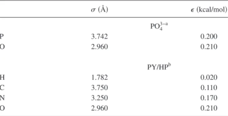
TABLE I. LJ parameters. ␴共Å兲 ⑀共kcal/mol兲 PO43−a P 3.742 0.200 O 2.960 0.210 PY/HPb H 1.782 0.020 C 3.750 0.110 N 3.250 0.170 O 2.960 0.210 a_Reference28. b_{References24,29, and30.}

TABLE II. Geometrical parameters of PO₄3−_{共Å兲in gas phase and in aqueous} solution.

Gas phase Aqueous solution

RISM-SCF-SEDD C-PCM Expt.a

geom I geom II geom III

P–O 1.582 1.539 1.556 1.53

O–O 2.583 2.514 2.541 2.49

Nt共r兲= 4␲␳tv

冕

0 r x2gXt共x兲dx 共X= P or O兲, 共16兲 where␳t V

is the number density of water. A high and narrow peak was seen at 1.69 Å ingOH_w共r兲, indicating a strong

hy-drogen bonding between O sites of PO₄3−and Hw. The P – Ow

peak at 3.67 Å was broad compared to O – H_wpeak. This is because O_wdoes not interact directly with PO₄3−and fluctu-ates around H_w. The peak position of RDF and coordination number obtained by RISM-SCF-SEDD is compared to the experimental data21 in Table III. The computed distances show a good agreement, especially the P – O_w distance is almost identical to the experiment data. The coordination numbers corresponding to the first shell are somewhat larger, but reasonably accord with those obtained by the neutron scattering experiments.

B. PY/HP

In this molecule, tautomeric isomerization occurs be-tween amide form共PY兲 and imidic acid forms共HP兲. Three conformers, PY, HPanti, and HPsynare considered in terms of

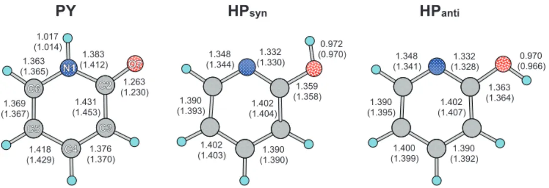
the position of the transferring H atom. Geometries of these conformers were optimized underCssymmetry and shown in

Fig. 2. The obtained geometry reasonably agrees with the experimental data determined by microwave spectroscopy.23 Root mean square deviation in the bond length between the DFT共B3LYP兲calculations and experimentally obtained data in gas phase was 0.015 Å for PY and 0.010 Å for HPsyn. The

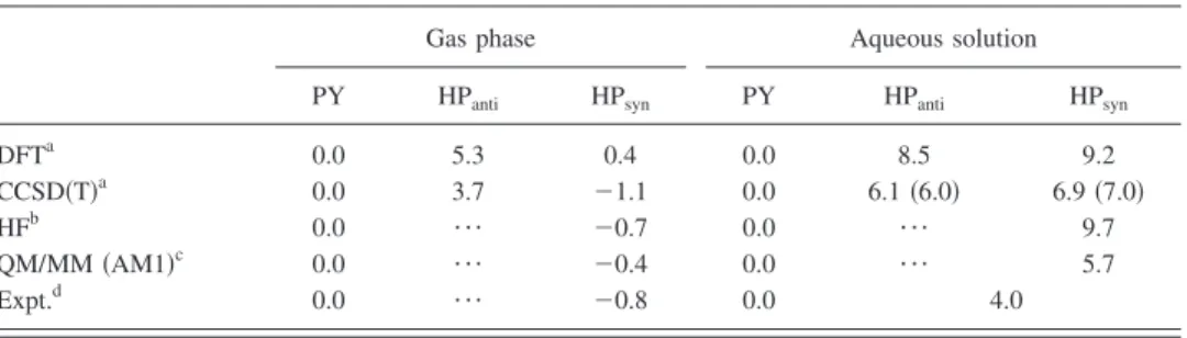
deviation is satisfactorily small, suggesting that calculation is reliable for the geometry optimization. On the other hand, much highly sophisticated quantum chemical method is nec-essary to adequately evaluate the relative energy. The energy obtained by DFT 共B3LYP兲shows that PY is slightly stable, contradicting the experimental data. By performing CCSD共T兲 calculation the relative stability between PY and HP was properly reproduced共TableIV兲.

The geometries in aqueous phase calculated by RISM-SCF-SEDD are also shown in Fig.2. The solvation does not affect the geometry of HP_synand HP_antiso much. The maxi-mum change in distances from gas to aqueous phase was only 0.004 Å for HPsynand 0.007 Å for HPanti. On the other

hand, the geometry of PY in aqueous phase is quite different from that in gas phase. In particular, the bond lengths of C2–N1 and C3–C2 decrease by 0.029 and 0.022 Å, respec-tively, and that of O7–C2 increases by 0.033 Å. This large change may be understood with resonance structures in PY. As shown in Scheme1, PY has zwitterionic resonance struc-tures in addition to amide form. In gas phase, amide form is stable compared to zwitterionic form, while the zwitterionic resonance structures are much stabilized in aqueous phase by solvent water. In aqueous phase, the double bond character becomes greater in C2–N1 and C3–C2 bonds while single bond character becomes greater in O7–C2 bond.

The relative free energy in aqueous phase calculated by the present method is shown in TableIV, where those com-puted by the original RISM-SCF 共HF level兲24 and by QM/MM 共Ref. 25兲are also shown. In the case of CCSD共T兲 calculation in aqueous phase, the energies were also evalu-ated with a different type of LJ parameter, general amber force field共GAFF兲.26A qualitative trend, namely, PY became more stable compared to HP in aqueous solution, is repro-duced by all methods, but there are quantitative differences among the methods. DFT level calculation with RISM-SCF-SEDD and the original RISM-SCF overestimate the stability

TABLE III. The RDF peak position and the coordination number. This work Expt.a

P – Owdistance共Å兲 3.67 3.7 O – Hwdistance共Å兲 1.69 1.9 N共first shell of P – Ow兲 18.4 15⫾3 N共first shell of O – Hw兲 5.2 3 a_Reference21. 0 2 4 6 8 0 2 4 6 8 0 5 10 15 20 g (r) r / angstrom N (r) g(r) N(r) P-Ow g(r) N(r) O-Hw

FIG. 1. Radial distribution functions关g共r兲兴and coordination numbers关N共r兲兴 of water oxygen 共O_w兲and water hydrogen 共H_w兲 around solute P and O atoms. PY 1.017 (1.014) 1.363 (1.365) 1.369 (1.367) 1.418 (1.429) 1.376 (1.370) 1.431 (1.453) 1.263 (1.230) N1 N1 C6 C6 O7 O7 1.383 (1.412) C5 C5 C4 C4 C3 C3 C2 C2 1.348 (1.344) 1.390 (1.393) 1.402 (1.403) _(1.390)1.390 1.402 (1.404) 1.332 (1.330) 1.359 (1.358) 0.972 (0.970) HPsyn 1.348 (1.341) 1.390 (1.395) 1.400 (1.399) (1.392)1.390 1.402 (1.407) 1.332 (1.328) 1.363 (1.364) 0.970 (0.966) HPanti

FIG. 2. Optimized bond lengths in PY, HPsyn, and HPanti共Å兲in aqueous phase. The values in gas phase are in parenthesis.

of PY. The agreement is certainly improved with the present RISM-SCF-SEDD coupled with CCSD共T兲calculation. In the calculation, the sensitivity of LJ parameters was significantly small.

Figure3 displays the radial distribution functions of hy-drogen共Hw兲 of solvent water around N and O atoms in the

three isomers obtained by RISM-SCF-SEDD method. In HPsyn and HPanti, the peak around 2 Å corresponds to the

hydrogen bonding. Hwcoordinates to both N and O atoms,

which are exposed to the solvent. In the case of PY, N atom is already occupied by the transferring H atom and Hw

can-not interact, leading to the disappearance of the peak around 2 Å seen in HP. At the same time, O atom in PY shows alkoxide character and its charge becomes more negative compared to that in HP. Consequently, O strongly attracts H_w, which makes RDF of O – H_whigher. This is an important factor that PY is strongly stabilized in aqueous phase. V. CONCLUSIONS

We derived an analytical energy gradient formula based on RISM-SCF-SEDD. The present method was applied to two demonstrative systems in aqueous phase, phosphate an-ion PO₄3−, and tautomerization between PY and HP.

The computational procedure of RISM-SCF-SEDD is numerically stable compared to the original RISM-SCF. The new method has expanded the applicability ofab initio elec-tronic structure calculation coupled with solvation effect and the development of energy gradient technique reported here further extends the capability of the method. It should be emphasized that both of the original SCF and RISM-SCF-SEDD methods are equivalent to ab initio QM/MM method, in which the electronic structure of the solute mol-ecule is determined under the influence of solvent molmol-ecules. Thanks to the analytical treatment based on statistical me-chanics, the computational time to evaluate the statistical en-semble is negligibly short. This feature enables us to com-bine highly sophisticated electronic structure theory, e.g.,

CCSD共T兲, DFT. We believe that the present method will be-come the powerful tools to analyzing interesting chemical systems, such as chemical reactions in solution, with reason-able computational cost.

ACKNOWLEDGMENTS

This work was financially supported in part by the Grant-in Aid for Scientific Research on Priority Areas “Water and Biomolecules” 共Grant No. 430-18031019兲, “Molecular Theory for Real Systems” 共Grant No. 461兲, “Ionic Liquids”

共Grant No. 452-20031014兲, “Molecular Science of Fluctua-tions”共Grant No. 2006-21107511兲, and by the Grant-in Aid for General Research共Grant No. 19350010兲. D.Y. thanks the Grant-in Aid for JSPS Fellows. All of them were supported by the Ministry of Education, Culture, Sports, Science and Technology 共MEXT兲Japan.

APPENDIX: DERIVATION OF EQUATION_„13_…

After some mathematical manipulation, the derivative of excess chemical potential⌬␮with respect to nuclear coordi-nateR_␣is obtained as follows:

TABLE IV. Computed and experimentally obtained relative energies共kcal/mol兲. The energies in aqueous phase calculated by CCSD共T兲with GAFF parameter are shown in parentheses.

Gas phase Aqueous solution

PY HPanti HPsyn PY HPanti HPsyn

DFTa 0.0 5.3 0.4 0.0 8.5 9.2 CCSD共T兲a 0.0 3.7 ⫺1.1 0.0 6.1共6.0兲 6.9共7.0兲 HFb 0.0 ¯ ⫺0.7 0.0 ¯ 9.7 QM/MM共AM1兲c 0.0 ¯ ⫺0.4 0.0 ¯ 5.7 Expt.d 0.0 ¯ ⫺0.8 0.0 4.0 a_{This work.} b_Reference24. c_Reference25. d_{References23,31, and32.} N O H N O H N O H

SCHEME 1. Resonance structures in PY.

0 1 2 3 4 5 6 0 2 4 6 PY HPsyn HPanti O - Hw N - Hw r / angstrom g(r)

FIG. 3. Radial distribution functions of water hydrogen共Hw兲around N and O atoms in PY, HPsyn, and HPanti.

⳵⌬␮ ⳵R_␣ = − 1 ␤

兺

␣,s ␳s V

冕

dr

冋

共e−␤␾␣s UV 共r_兲+t_␣UV_s共r_兲 − 1 −h_␣s UV_共 r兲兲 ⫻⳵t␣s UV_共 r兲 ⳵Ra +共−t_␣s UV_共 r兲+h_␣s UV_共 r兲−c_␣s UV_共 r兲兲⳵h␣s UV_共 r兲 ⳵Ra +

冉

−h_␣s UV_共 r兲+

兺

␥t ␻␣␥Uc␥s UV_␹ st VV_共 r兲

冊

⳵c␣s UV_共 r兲 ⳵Ra +共−␤e−␤␾␣s UV_共r兲 +t_␣UV_s兲⳵␾␣s UV ⳵Ra +

冉

1 2

兺

_␥t ⳵␻␣␥U ⳵Ra c_␣s UV c_␥t UV_␹ st VV_共 r兲

冊

册

. 共A1兲 The terms with the derivatives oftUV_,hUV_{, andc}UV_are

van-ished using RISM and HNC equations. Because the distance r between solute and solvent atoms in the solute-solvent interaction potential 兵␾_␣s

UV_其

does not depend on the nuclear coordinates R_␣ of solute atoms, the derivative of ␾_␣s

UV in Eq.共A1兲is given by ⳵␾␣s UV ⳵Ra = −qs

兺

i_苸␣ ⳵di ⳵R_␣

冕

fi共r

⬘

兲 兩r−r

⬘

兩dr

⬘

. 共A2兲

By substituting Eq.共A2兲into Eq.共A1兲, Eq.共13兲is obtained.

1_{J. Tomasi, B. Mennucci, and R. Cammi,Chem. Rev.共Washington, D.C.兲} 105, 2999共2005兲.

2_{R. Cammi and J. Tomasi,J. Chem. Phys. 100, 7495共1994兲; 101, 3888} 共1994兲; M. Cossi, B. Mennucci, and R. Cammi,J. Comput. Chem.17, 57 共1996兲.

3_{P. Bandyopadhyay, M. S. Gordon, B. Mennucci, and J. Tomasi,J. Chem.} Phys. 116, 5023共2002兲.

4_{N. Okuyama-Yoshida, K. Kataoka, M. Nagaoka, and T. Yamabe, J.} Chem. Phys. 113, 3519共2000兲.

5_{M. E. Martín, A. M. Losa, I. Fdez Galván, and M. A. Aguilar,J. Chem.} Phys. 121, 3710共2004兲.

6_{Molecular Theory of Solvation, edited by F. Hirata共Kluwer, Dordrecht,} 2003兲.

7_{S. Ten-no, F. Hirata, and S. Kato,J. Chem. Phys. 100, 7443共1994兲.} 8_{H. Sato, F. Hirata, and S. Kato,J. Chem. Phys. 105, 1546共1996兲.} 9_{S. Hayaki, K. Kido, D. Yokogawa, H. Sato, and S. Sakaki,J. Phys. Chem.}

B 113, 8227共2009兲.

10_{K. Iida, D. Yokogawa, A. Ikeda, H. Sato, and S. Sakaki,Phys. Chem.} Chem. Phys. 11, 8556共2009兲; K. Iida, D. Yokogawa, H. Sato, and S. Sakaki,Chem. Phys. Lett. 443, 264共2007兲.

11_{D. Yokogawa, H. Sato, and S. Sakaki, J. Chem. Phys. 126, 244504} 共2007兲.

12_{S. J. Singer and D. Chandler,Mol. Phys. 55, 621共1985兲.} 13_{S. Obara and A. Saika,J. Chem. Phys. 84, 3963共1986兲.} 14_{R. Ahlrichs,Phys. Chem. Chem. Phys. 8, 3072共2006兲.}

15_{M. W. Schmidt, K. K. Baldridge, J. A. Boatz, S. T. Elbert, M. S. Gordon,} J. H. Jensen, S. Koseki, N. Matsunaga, K. A. Nguyen, S. Su, T. L. Windus, M. Dupuis, and J. A. Montgomery,J. Comput. Chem. 14, 1347 共1993兲.

16_{Useful libraries for FFT calculation can be download from the following} web page:http://www.kurims.kyoto-u.ac.jp/~ooura/.

17_{A. Kovalenko, S. Ten-no, and F. Hirata, J. Comput. Chem. 20, 928} 共1999兲.

18_{CCSD共T兲calculation in this work was performed using the subroutine} implemented inGAMESS共Ref.27兲.

19_{V. Barone and M. Cossi,J. Phys. Chem. A 102, 1995共1998兲.} 20_{H. J. C. Berendsen, J. P. M. Postma, W. F. van Gunsteren, and J.}

Her-mans, inIntermolecular Forces, edited by B. Pullman共Reidel, Dordrecht, 1981兲.

21_{P. E. Mason, J. M. Cruickshank, G. W. Neilson, and P. Buchanan,Phys.} Chem. Chem. Phys. 5, 4686共2003兲.

22_{To check the accuracy of the present calculation level, the optimized} distances were also computed by RISM-SCF-SEDD with CCSD共T兲. Be-cause analytical gradient of CCSD共T兲was not available in the current version ofGAMESSpackage, the optimized geometry was determined nu-merically by evaluating free energy surface. The obtained distances were 1.536 Å for P–O and 2.507 Å for O–O, which are very close to those obtained by DFT共B3LYP兲calculation.

23_{L. D. Hatherley, R. D. Brown, P. D. Godfrey, and A. P. Pierlot,J. Phys.} Chem. 97, 46共1993兲.

24_{H. Sato, F. Hirata, and S. Sakaki,J. Phys. Chem. A 108, 2097共2004兲.} 25_{J. Gao and L. Shao,J. Phys. Chem. 98, 13772共1994兲.}

26_{J. Wang, R. M. Wolf, J. W. Caldwell, P. A. Kollman, and D. A. Case,J.} Comput. Chem. 25, 1157共2004兲.

27_{P. Piecuch, S. A. Kucharski, K. Kowalski, and M. Musial,Comput. Phys.} Commun. 149, 71共2002兲.

28_{W. D. Cornell, P. Cieplak, C. I. Bayly, I. R. Gould, K. M. Merz, Jr., D. M.} Ferguson, D. C. Spellmeyer, T. Fox, J. W. Caldwell, and P. A. Kollman, J. Am. Chem. Soc. 117, 5179共1995兲.

29_{W. L. Jorgensen and J. Tirado-Rives, J. Am. Chem. Soc. 110, 1657} 共1988兲.

30_{S. J. Weiner, P. A. Kollman, D. A. Case, U. C. Singh, C. Ghio, G.} Alagona, S. Profeta, Jr., and P. Weiner, J. Am. Chem. Soc. 106, 765 共1984兲.

31_{P. Beak,Acc. Chem. Res. 10, 186共1977兲.}

32_{J. Frank and A. R. Katritzky,J. Chem. Soc., Perkin Trans. 2 1976, 1428.}