DISTRIBUTED CLUSTER PRUNING IN HADOOP

(1)

ISSN 1670-8539

M.Sc. PROJECT REPORT

Andri Mar Björgvinsson

Master of Science

Computer Science

May 2010

School of Computer Science

Reykjavík University

(2)

(3)

Project Report Committee:

Björn Þór Jónsson, Supervisor

Associate Professor, Reykjavík University, Iceland

Magnús Már Halldórsson

Professor, Reykjavík University, Iceland

Hjálmtýr Hafsteinsson

Associate Professor, University of Iceland, Iceland

Project report submitted to the School of Computer Science

at Reykjavík University in partial fulfillment of

the requirements for the degree of

Master of Science

in

Computer Science

(4)

Copyright

Andri Mar Björgvinsson

May 2010

(5)

Abstract

Clustering is a technique used to partition data into groups or clusters based

on content. Clustering techniques are sometimes used to create an index from

clusters to accelerate query processing. Recently the cluster pruning method

was proposed which is a randomized clustering algorithm that produces

clus-ters and an index both efficiently and effectively. The cluster pruning method

runs in a single process and is executed on one machine. The time it takes to

cluster a data collection on a single computer therefore becomes

unaccept-able due to increasing size of data collections.

Hadoop is a framework that supports data-intensive distributed applications

and is used to process data on thousands of computers. In this report we adapt

the cluster pruning method to the Hadoop framework. Two scalable

dis-tributed clustering methods are proposed: the Single Clustered File method

and the Multiple Clustered Files method. Both methods were executed on

one to eight machines in Hadoop and were compared to an implementation

of the cluster pruning method which does not execute in Hadoop. The results

show that using the Single Clustered File method with eight machines took

only 15% of the time it took the original cluster pruning method to cluster

a data collection while maintaining the cluster quality. The original method,

however, gave slightly better search time when compared to the execution of

the Single Clustered File method in Hadoop with eight nodes. The results

indicate that the best performance is achieved by combining the Single

Clus-tered File method for clustering and the original method, outside of Hadoop,

for searching. In the experiments, the input to both methods was a text file

with multiple descriptors, so even better performance can be reached by

us-ing binary files.

(6)

Cluster Pruning dreifð með Hadoop

Andri Mar Björgvinsson

Maí 2010

Útdráttur

Þyrping gagna (e. clustering) er aðferð þar sem gögn er hafa svipaða

eigin-leika eru sett saman í hóp. Til eru nokkrar aðferðir við þyrpingu gagna,

sumar þessarra aðferða búa einnig til vísi sem er notaður til þess að hraða

fyrirspurnum. Nýleg aðferð sem heitir „cluster pruning” velur af handahófi

punkta til þess að þyrpa eftir og býr jafnframt til vísi yfir þyrpingarnar. Þessi

aðferð hefur skilað góðum og skilvirkum niðurstöðum bæði fyrir þyrpingu

og fyrirspurnir. Cluster pruning aðferðin er keyrð á einni vél. Sá tími sem

tekur eina vél að skipta gagnasafni upp í hópa er að lengjast þar sem

gagna-söfnin eru sífellt að stækka. Því er þörf á að minnka vinnslutímann svo að

hann sé innan ásættanlegra marka.

Hadoop er kerfi sem styður hugbúnað er vinnur með mikið magn af gögnum.

Hadoop kerfið dreifir vinnslunni á gögnunum yfir margar vélar og flýtir þar

með keyrslu hugbúnaðarins. Í þessu verkefni var cluster pruning aðferðin

aðlöguð að Hadoop kerfinu. Lagðar voru fram tvær aðferðir sem byggja á

cluster pruning aðferðinni; Single Clustered File aðferð og Multiple

Clus-tered Files aðferð. Báðar aðferðirnar voru keyrðar á einni til átta tölvum

í Hadoop kerfinu og þær bornar saman við upprunalega afbrigðið af cluster

pruning sem er ekki keyrt í Hadoop kerfinu. Niðurstöður sýndu að þegar

Sin-gle Clustered File aðferðin var keyrð á átta tölvum þá tók það aðeins 15% af

tímanum sem það tók upprunalega cluster pruning aðferðina að þyrpa gögnin

og jafnframt náði hún að viðhalda sömu gæðum. Upprunalega cluster

prun-ing aðferðin gaf örlítið betri leitartíma þegar hún er borin saman við keyrslu

á Single Clustered File aðferðinni í Hadoop þegar notast var við átta tölvur.

Rannsóknin sýnir að með því að nota saman Single Clustered File method

við þyrpingu gagna og upprunalega afbrigðið af cluster pruning við leit, án

Hadoop, þá nást bestu afköstin. Við prófanir voru báðar aðferðirnar að vinna

með textaskrár en hægt væri að ná betri tíma við þyrpingu gagna með því að

nota tvíundaskrár (e. binary files).

(7)

Acknowledgements

I wish to thank Grímur Tómas Tómasson and Haukur Pálmason for supplying me with the code for the original cluster pruning method, and for their useful feedback on this project. I would also like to thank my supervisor Björn Þór Jónsson for all the support during this project.

(8)

(9)

List of Figures

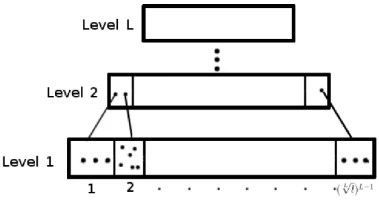
2.1 The index withLlevels andlrepresentatives in the bottom level . . . 7 3.1 Execution of the word count example. . . 11 5.1 Clustering using MCF, SCF, and the original method. . . 22 5.2 Search time for 600 images using SCF, MCF and the original method. . . 24 5.3 Vote ratio for 100 derived images using SCF, MCF and the original method.

(12)

(13)

List of Tables

(14)

(15)

List of Abbreviations

The following variables are used in this report. Category Variable Description

Clustering p Image descriptor (SIFT), a point in 128-dimensional space

S Set of descriptors for an image collection

nS Number of descriptors inS

L Number of levels in the cluster index

l Number of clusters in the index

ri Representative of clusteri,0< i≤l

vi Number of descriptors in clusteri

Searching q Query descriptor

Q Set of query descriptors

nQ Number of descriptors inQ

k Number of nearest neighbors to retrieve for each query descriptor

b Number of clusters to scan for each query descriptor

t Number of result images to return for each query image

Hadoop C Number of computers in the Hadoop cluster

M Number of 64MB chunks in the descriptor collection

(16)

(17)

Chapter 1 Introduction

The size of multimedia collections is increasing and with it the need for fast retrieval. There is much research on nearest neighbor search in high-dimensional spaces. Most of those methods take the data collection (text,images...) and convert them into a collection of descriptors with multiple dimensions. The collection of descriptors is then segmented into groups and stored together on disk. An index is typically created to accelerate query processing.

Several indexing methods have been proposed, such as the NV-Tree [8] and LSH [2]. They create an index which is used to query the data collection, resulting in fewer com-parisons of data points. By using a good technique for indexing, the disk reads can be minimized. The number of disk reads can make a significant difference when working with a large disk-based data collection.

1.1 Clustering

Clustering is a common technique for static data analysis and is used in many fields, such as machine learning, data mining, bioinformatics and image analysis. Typically these methods identify the natural clusters of the data collection. K-means clustering is a good example of such a method. K-means attempts to find the center of a natural cluster by recursively clustering a data collection and finding a new centroid each time; this is repeated until convergence has been reached.

Chierichetti et al. proposed a method called “cluster pruning” [1]. Cluster pruning con-sists of selecting random cluster leaders from a set of points, and the rest of the points are then clustered based on which cluster leader they are closest to. Guðmundsson et al.

(18)

2 Distributed Cluster Pruning in Hadoop

studied cluster pruning in the context of large-scale image retrieval and proposed some extensions [6].

All these methods have been designed to work in a single process, so clustering a large dataset can take a long time. One way to cluster a large dataset in multiple processes is to use distributed computing and cluster data in parallel. Parallel processing of data has shown good results and can decrease processing time significantly. Manjarrez-Sanchez et al. created a method that runs nearest neighbor queries in parallel by distributing the clus-ters over multiple machines [9]. They did not, however, provide any distributed clustering method.

1.2 Hadoop

The Hadoop distributed file system (HDFS) is a tool to implement distributed computing and parallel processing for clustering and querying data collections. Processing large datasets with Hadoop has shown good results. Hadoop is a framework that supports data-intensive distributed applications; it allows applications to run on thousands of computers and can decrease processing time significantly. Hadoop has been used to solve a variety of problems with distributed computing, for example, machine translation on large data [4, 10, 11] and estimating the diameter of large graphs [7].

HDFS was inspired by two sysems from Google, MapReduce [3] and Google File Sys-tem (GFS) [5]. GFS is a scalable distributed file sysSys-tem for data-intensive applications and provides a fault tolerant way to store data on commodity hardware. GFS can de-liver high aggregate performance to a large number of clients. The MapReduce model, created by Google, provides a simple and powerful interface that enables automatic par-allelization and distribution of large computations on commodity PCs. The GFS provides MapReduce with distributed storage and high throughput of data. Hadoop is the open source implementation of GFS and MapReduce.

1.3 Contribution

The contribution of this paper is to adapt the cluster pruning method to MapReduce in Hadoop. We propose two different methods for implementing clustering and search in parallel using Hadoop. We then measure the methods on an image copyright protection workload. By using Hadoop on only eight computers, the clustering time of a data

(19)

collec-method, while Section 3 reviews the Hadoop system. Section 4 presents the adaptation of cluster pruning to Hadoop. Section 5 presents the results from the performance ex-periments and in Section 6 we arrive at a conclusion as to the usability of the proposed methods.

(20)

(21)

Chapter 2 Cluster Pruning

There are two phases to cluster pruning. First is the clustering phase, where random cluster representatives are selected, the data collection is clustered and cluster leaders are selected. An index with L levels is created by recursively clustering the cluster lead-ers.

Next is the query processing phase, where the index is used to accelerate querying. By using the index, a cluster is found for each query descriptor and this cluster is searched for the nearest neighbor.

2.1 Clustering

The input to cluster pruning is a set S of nS high-dimensional data descriptors, S =

{p1, p2....pnS}. Cluster pruning starts by selecting a set ofl =

√

nS random data points

r1, r2...r√nS, from the set of descriptorsS. Theldata points are called cluster

represen-tatives.

All points inS are then compared to the representatives and a subset from S is created for every representative. This subset is described by[ri,{pi1, pi2....piv}], wherev is the number of points in the cluster withri as the nearest representative. This means that data

points inS will be partitioned intolclusters, each with one representative.

Chierichetti et al. proposed using√nS representatives, since that number minimizes the

number of distance comparisons during search, and is thus optimal in main-memory sit-uations. But Guðmundsson et al. studied the cluster pruning method and its behavior in an image indexing context at a much larger scale [6]. That study revealed that using

l=d nS

(22)

default IO granularity of the Linux operating system) gave better results when working on large data collections. This value oflresults in fewer but larger clusters and a smaller index, which gave better performance in a disk-based setting.

For alll clusters, a cluster leader is then selected. The leader is used to guide the search to the correct cluster. Chierichetti et al. considered three ways to select a cluster leader for each cluster:

1. Leaders are the representatives.

2. Leaders are the centroids of the corresponding cluster.

3. Leaders are the medoids of each cluster, that is the data point closest to the centroid. Chierichetti et al. concluded that using centroids gave the best results [1]. Guðmundsson et al. came to the conclusion, however, that while using the centroids may give slightly better results than using the representatives, the difference in clustering time is so dramatic that it necessitates the use of representatives instead of centroids as cluster leaders [6]. Using the representatives as cluster leaders means that the bottom level in the cluster index is known before image descriptors are assigned to representatives. The whole cluster index can therefore be created before the insertion of image descriptors to the cluster. Thus the index can be used to cluster the collection of descriptors, resulting in less time spent on clustering.

The cluster pruning method can, recursively in this case, cluster the set of cluster leaders using the exact same method as described above. L is the number of recursions, which controls the number of levels in the index. An index is built, where the bottom level contains thel cluster leaders from clusteringS as described above. (√Ll)L−1 _descriptors

are then chosen from the bottom level to be the representatives for the next level in the index. This results in a new level with √Llfewer descriptors than the bottom level. The rest of the descriptors from the bottom level are then compared to the new representatives and partitioned into(√Ll)L−1 clusters. This process is repeated until the top level is reached. Figure 2.1 shows the index after recursively clustering the representatives. This can be thought of as building a tree, resulting in fewer distance calculations when querying a data collection. Experiments in [6] showed that usingL= 2gave the best performance. Chierichetti et al. also defined parametersaandb. Parameteragives the option of assign-ing each point to more than one cluster leader. Havassign-inga > 1will lead to larger clusters due to replication of data points. Parameter b, on the other hand, specifies how many nearest cluster leaders to use for each query point.

(23)

Figure 2.1: The index withLlevels andlrepresentatives in the bottom level Guðmundsson et al. showed that the parameter a is not viable for large-scale indexing and that usinga = 1gave the best result. Tuningb, on the other hand can result in better result quality. However, incrementing b from 1 to 2, resulted in less than 1% increase in quality while linearly increasing search time [6]. In this paper we will therefore use

b= 1, because of this relatively small increase in quality.

2.2 Searching

In query processing, a set of descriptors Q = {q1, q2...qs} is given from one or more

images.

First the index file is read. For each descriptor qi in the query file the index is used

to find which b clusters to scan. The top level of the index is, one by one, compared to all descriptors in Q and the closest representatives found for each descriptor. The representatives from the lower level associated with the nearest neighbor from the top level are compared to the given descriptor, and so on, until reaching the bottom level. When the bottom level is reached, theb nearest neighbors there are found. Theb nearest neighbors from the bottom level represent the clusters where the nearest neighbors ofqi

are to be found.

Qis then ordered based on which clusters will be searched for eachqi; query descriptors

with search clusters in the beginning of the clustered file are processed first. By ordering

Q, it is possible to read the clustered descriptor file sequentially and search only those clusters needed byQ. Forqi thek nearest neighbors in theb clusters are found and the

(24)

images that these descriptors belong to receive one vote. After this is done, the vote results are aggregated, and the image with the highest number of votes is considered the best match.

(25)

Chapter 3 Hadoop

Hadoop is a distributed file system that can run on clusters ranging from a single computer up to many thousands of computers. Hadoop was inspired by two systems from Google, MapReduce [3] and Google File System [5].

GFS is a scalable distributed file system for data-intensive applications. GFS provides a fault tolerant way to store data on commodity hardware and deliver high aggregate performance to a large number of clients.

MapReduce is a toolkit for parallel computing and is executed on a large cluster of com-modity machines. There is quite a lot of complexity involved when dealing with par-allelizing the computation, distributing data and handling failures. Using MapReduce allows users to create programs that run on multiple machines but hides the messy details of parallelization, fault-tolerance, data distribution, and load balancing. MapReduce con-serves network bandwidth by taking advantage of how the input data is managed by GFS and is stored on the local storage device of the computers in the cluster.

3.1 Google File System

In this section, the key points in the Google File System paper will be reviewed [5]. A GFS consists of a single master node and multiple chunkservers. Files are divided into multiple chunks; the default chunk size is 64MB, which is larger than the typical file system block size. For reliability, the chunks are replicated on to multiple chunkservers depending on the replication level given to the chunk upon creation; by default the replica-tion level is 3. Once a file is written to GFS, the file is only read or mutated by appending new data rather than overwriting existing data.

(26)

The master node maintains all file metadata, including the namespace, mapping from files to chunks, and current location of chunks. The master node communicates with each chunkserver in heartbeat messages to give it instructions and collect its state. Clients that want to interact with GFS only read metadata from the master. Clients ask the master for the chunk locations of a file and directly contact the provided chunkservers for receiving data. This prevents the master from becoming a major bottleneck in the system.

Having a large chunk size has its advantages. It reduces the number of chunkservers the clients need to contact for a single file. It also reduces the size of metadata stored on the master, which may allow the master to keep the metadata in memory.

The master does not keep a persistent record of which chunkservers have a replica of a given chunk; instead it pulls that information from the chunkservers at startup. After startup it keeps itself up to date with regular heartbeat messages, updates the location of chunks, and controls the replication. This eliminates the problem of keeping the master and chunkservers synchronized as chunkservers join and leave the cluster. When inserting data to the GFS, the master tells the chunkservers where to replicate the chunks; this position is based on rules to keep the disk space utilization balance.

In GFS, a component failure is thought of as the norm rather than exception, and the system was built to handle and recover from these failures. Constant monitoring, error detection, fault tolerance, and automated recovery is essential in the GFS.

3.2 MapReduce

In this section the key points of the MapReduce toolkit will be reviewed [3].

MapReduce was inspired by the map and reduce primitives present in Lisp and other functional languages. The use of the functional model allows MapReduce to parallelize large computation jobs and re-execute jobs that fail, providing fault tolerance.

The interface that users must implement contains two functions, map and reduce. The map function takes an input pair< K1, V1 >and produces a new key/value pair< K2, V2 >.

The MapReduce library groups the key/value pairs produced and sends all pairs with the same key to a single reduce function. The reduce function accepts list of values with the same key and merges these values down to a smaller output; typically one or zero outputs are produced by each reducer.

(27)

Figure 3.1: Execution of the word count example.

Consider the following simple word count example, where the pseudo-code is similar to what user would write:

map (String key,String value)

//key is the document name. //value is the document content.

for eachwinvalue: emitKeyValue (w, "1")

reduce (String key,String[]value)

//key is a word from the map function. //value is a list of values with the same key.

intcount= 0 for eachcinvalue:

count += int(c) emit(key, str(count))

In this simple example, themapfunction emits each word in a string, all with the value one. For each distinct word emitted, thereduce function sums up all values, effectively counting the number of occurrences. Figure 3.1 shows the execution of the word count pseudo-code on a small example text file.

The run-time system takes care of the details of partitioning the the input data, scheduling the MapReduce jobs over multiple machines, handling machine failures and re-executing MapReduce jobs.

(28)

When running a MapReduce job, the MapReduce library splits the input file into M

pieces, where M is the input file size divided by the chunk size of the GFS. One node in the cluster is selected to be a master and the rest of the nodes are workers. Each worker is assigned map tasks by the master, which sends a chunk of the input to the worker’s map function. The new key/value pairs from the map function are buffered in memory.

Periodically, the buffered pairs are written to local disk and partitioned in regions based on the key. The location of the buffered pairs is sent to the master, which is responsible for forwarding these locations to the reduce workers. Each reduce worker is notified of the location by the master and uses remote procedure calls to read the buffered pairs.

For each complete map task, the master stores the location and size of the map output. This information is pushed incrementally to workers that have an in-progress reduce task or are idle.

The master pings every worker periodically; if a worker does not answer in a specified amount of time the master marks the worker as failed. If a map worker fails, the task it was working on is re-executed because map output is stored on local storage and is therefore inaccessible.

The buffered pairs with the same key are sent as a list to the reduce functions. Each reduce function iterates over all the key/value pairs and the output from the reduce function is appended to a final output file.

Reduce invocations are distributed and one reduce function is called per key, but the number of partitions is decided by the user. If the user only wants one output, one instance of a reduce task is created. The reduce function in the reduce task is called once per key. Selecting a smaller number of reduce tasks than the number of nodes in the cluster will result in only some, and not all, of the nodes in the cluster being used to aggregate the results of the computation. Reduce tasks that fail do not need to be re-executed, just the last record, since their output is stored in the global file system.

When the master node is assigning jobs to workers, it takes into account where replicas of the input chunk are located and makes a worker running on one of those machines process the input. In case of a failure in assigning a job to the workers containing the replica of the input chunk, the master assigns the job to a worker close to the data (same network switch or same rack). When running a large MapReduce job, most of the input data is read locally and consumes no network bandwidth.

MapReduce has a general mechanism to prevent so-called stragglers from slowing down a job. When a MapReduce job is close to finishing it launches a backup task to work on

(29)

sent to the reducers and can significantly speed up certain classes of MapReduce opera-tions.

3.3 Hadoop Core System

MapReduce [3] and the Hadoop File System (HDFS), which is based on GFS [5], is what defines the core system of Hadoop. MapReduce provides the computation model while HDFS provides the distributed storage. MapReduce and HDFS are designed to work together. While MapReduce is taking care of the computation, HDFS is providing high throughput of data.

Hadoop has one machine acting as a NameNode server, which manages the file system namespace. All data in HDFS are split up into block sized chunks and distributed over the Hadoop cluster. The NameNode manages the block replication. If a node has not answered for some time, the NameNode replicates the blocks that were on that node to other nodes to keep up the replication level.

Most nodes in a Hadoop cluster are called DataNodes; the NameNode is typically not used as a DataNode, except for some small clusters. The DataNodes serve read/write requests from clients and perform replication tasks upon instruction by NameNode. DataNodes also run a TaskTracker to get map or reduce jobs from JobTracker.

The JobTracker runs on the same machine as NameNode and is responsible for accepting jobs submitted by users. The JobTracker also assigns Map and Reduce tasks to Task-Trackers, monitors the tasks and restarts the tasks on other nodes if they fail.

(30)

(31)

Chapter 4 Methods

This chapter describes how cluster pruning is implemented within Hadoop MapReduce. We propose two methods which differ in the definition of the cluster index.

The first method is the Single Clustered File method (SCF). This method creates the same index over multiple machines and builds a single clustered file; both files are stored in a shared location. With this method the index and clustered file are identical to the ones in the original method, and each query descriptor can be processed on a single machine. The SCF method is presented in Section 4.1.

The second method is the Multiple Clustered Files method (MCF). In this method each worker creates its own index and clustered file, and both files are stored on its local stor-age. With this method, each local index is smaller, but each query descriptor must be replicated to all workers during search. The MCF is presented in Section 4.2.

Note that while the original implementation used binary data [6], Hadoop only supports text data by default. The implementation was therefore modified to work with text data. This is discussed in Section 4.3.

4.1 Single Clustered File (SCF)

This method creates one index per map task. All map tasks read sequentially the same file with descriptors, resulting in the same index over all map tasks. After clustering, all map tasks send the clustered descriptors to the reducers that write temporary files to a shared location. When all reducers are finished, the temporary files are merged by a process outside of the Hadoop System, resulting in one index and one clustered file in a shared location.

(32)

4.1.1 Clustering

This method has a map function, reduce function and a process outside of Hadoop, for combining temporary files.

When a map task is created, it starts by reading a file with descriptors, one descriptor per line. This file contains the representatives and is read sequentially. The file contains a collection of descriptors randomly selected from the whole input database and thus there is no need for random selection. This file is kept at a location that all nodes in the cluster can read from. When the map task is finished readingldescriptors from the file it can start building the index. The selected descriptors from the file containing the representatives make up the bottom level of the index. The level above is selected sequentially from the lower level.

After sequentially reading the randomized file containing the representatives, there are no more random selections. This is done so that all map tasks end up with the same index and would put identical descriptors in the same cluster. When a map task is finished creating an index, the index is written to a shared location for the combine method to use later. After the index is built and saved, the map function is ready to receive descriptors. The nearest neighbor in the bottom level of the index is found for all descriptors in the chunk, as described in Section 2.2. When the nearest neighbor is found for a descriptor we know which cluster this descriptor belongs to. After the whole chunk has been processed, the descriptors are sent to the reducer with information on which cluster they belong to.

The reducer goes through descriptors and writes them to temporary files in a shared loca-tion where the JobTracker is running. One temporary file is created per cluster. When all reducers have finished writing temporary files, a process of combining these files and up-dating the index is executed outside of the Hadoop system. The combining process reads the index saved by the map task. While the process is combining the temporary files to a single file, it updates the bottom level of the index. The bottom level of the index contains the number of descriptors within the clusters and where each cluster starts and ends in the combined file.

When this process is complete there is one clustered file and one index on shared storage and it is ready for search.

(33)

clustered descriptors and index file. When all this information has been read, the map function is ready to receive descriptors. The map function gathers descriptors until all descriptors have been distributed between the map tasks. Each map task creates a local query file for the combiner to use.

When the local query file is ready, the combiner can start by reading the local query and index file. The combiner can now start searching the data collection as described in Section 2.2.

The reduce function receives a chunk of results from the combiner, ortresults per query image. The same identifier might appear more than once in the query results for one image and the values must be combined for all image identifiers. The reducer then writes the results to an output file in the Hadoop system after each query identifier.

The map task runs on all workers but it is possible to limit the number of reduce tasks; if only one output file is required, one reduce task is executed. One reducer will give one output, ifRreducers are executed then the output is split intoRpieces.

4.2 Multiple Clustered Files (MCF)

This method also creates one index per map task. With this method, however, the index is smaller, as each worker only indexes a part of the collection. Each node builds its own index and clustered file and saves them locally. After clustering, all nodes running TaskTracker should have a distinct clustered file containing its part of the input file and an identical index file in local storage.

4.2.1 Clustering

In this method we have a map function, a combine function and a reduce function. The map functions is similar to the one in the SCF method, but there are two main differences between the two functions.

(34)

The first difference is the size ofl. In the MCF methodlis divided byC(lM CF =lSCF/C)

whereCis the number of nodes that will be used to cluster the data. Thus, the index isC

times smaller, because each node receives on averagen/C descriptors.

The second difference is that instead of sending the descriptors and information to the reducer, the map function sends it to the combiner. The combiner writes the descriptors to temporary files; one temporary file is created for each cluster. Using the combiner to write temporary files reduces the number of writes to a single write in each map task, instead of writing them once per chunk. When all records have been processed, a single reduce operation is executed on all nodes.

The reducer reads the index saved by the map task and while the reducer is combining the temporary files to a single file in local storage, the reducer updates the bottom level of the index. When the reducer is done combining temporary files and saving the index on local storage, both files are ready for querying.

4.2.2 Searching

After clustering descriptors with the MCF method, all nodes running TaskTracker should have their own small clustered file and an index. The Map task reads the configuration file that holds information about the configuration parameters such ask, b, and,tas well as the location of the query file.

When the map task has received this information, it can start searching the clustered data. The map function is the same as the combine function in SCF. However, all nodes have a replica of the whole query file that is used to query the clustered data, while the SCF method had a different part of the query file on all nodes.

The reduce function receives a chunk of results from all map tasks, ort×C results per image query identifier. As in the SCF method, the reducer adds up the votes for each image identifier and writes the results to an output file in the Hadoop system after every query.

4.3 Implementation

The input files are uploaded to HDFS, which replicates the files between DataNodes ac-cording to the replication level. The input consists of text files with multiple descriptors

(35)

All dimensions in each descriptor must be converted from a string to a byte (char) rep-resenting that number. This has some impact on the processing time; better performance can be obtained by having the input data as binary. Running the original cluster pruning with binary input was three times faster than running it on text file input. Some exten-sions to the Hadoop framework are needed, however, so that it can process binary files. A custom FileInputFormat, FileOutputFormat, record reader and record writer are needed for Hadoop to process binary data. This is an interesting direction for future work. All programming of the cluster pruning method was done in C++ and HadoopPipes was used to execute the C++ code within the Hadoop MapReduce framework. SSE2 was used for memory manipulation, among other features, and Threading Building Blocks (TBB) for local parallelism.

(36)

(37)

Chapter 5 Performance Experiments

5.1 Experimental Setup

In the performance experiments, Hadoop 0.20.2 was used with the Rocks 5.3 open-source Linux cluster distribution. Hadoop was running on one to eight nodes. Each node is a Dell precision 490. Note that there was some variance in the hardware; Table 5.1 shows the specification of all the nodes.

Nodes were added to the Hadoop cluster sequentially. When the data collection is up-loaded to the Hadoop file system (HDFS) it is automatically replicated to all DataNodes in Hadoop, as the replication level is set to the number of current DataNodes. When the data is replicated, MapReduce automatically distributes the work and decides how the im-plementation utilizes the HDFS. The time it took Hadoop to replicate the image collection to all nodes was 7.5 minutes.

The image collection that was clustered in this performance experiments contains 10,000 images or 9,639,454 descriptors. We used two query collections. One was a collection

Table 5.1: Specification for all machines.

Node RAM Cores CPUs Mhz

0 4 GB 8 3192 1 4 GB 4 2992 2 4 GB 4 2660 3 4 GB 4 1995 4 8 GB 8 3192 5 4 GB 4 1995 6 4 GB 4 2993 7 4 GB 8 2660

(38)

Figure 5.1: Clustering using MCF, SCF, and the original method.

with 600 images, where 100 were contained in the clustered data collection and the re-maining 500 were not. This collection was used to test the query performance on a number of nodes. The second query collection contained 100 images, where twenty images were modified in five different ways. This collection was used to test the search quality and get the vote ratio for the correct image. In all cases, the search found the correct image. The vote ratio was calculated by dividing the votes of the top image in the query result (the correct image) with the votes of the second image.

5.2 Clustering

This section contains the performance results for the clustering. Figure 5.1 shows the clustering time for each method depending on the number of nodes. Thex-axis shows the number of nodes and they-axis shows the clustering time, in seconds.

The difference in clustering time between the original method and a single node in a Hadoop-powered cluster, which is 9% for the SCF method and 13% for the MCF method, is the overhead of a job executed within Hadoop. The difference stems from Hadoop

(39)

is a 60% decrease in clustering time. The decrease in clustering time is not only because the number of nodes was doubled, but also because the index is only half of what it used to be, resulting in fewer comparisons when clustering a descriptor. The time it takes to cluster the data collection with the SCF method is almost cut in half, or by 47% from two computers to four. The reason that the clustering time does not decrease as much as with the MCF method is that the index size stays the same. The reduction in clustering time, when going from one node to two nodes, is even steeper. This my be explained by memory effects, as the descriptor collection barely fits within the memory of one node, but easily with in the memory of two nodes.

While using 1-3 nodes we can see in Figure 5.1 that the SCF method is faster. When the number of nodes is increased, the MCF method starts performing better when it comes to clustering time. Applying eight nodes to both methods resulted in 38% less time spent clustering with the MCF method, compared to the SCF method.

In the SCF method, there will be a bottleneck when more computers are added, because the clustered data is combined and all reducers are writing temporary files to the same storage device, while the MCF method is only writing to local storage and therefore scales better.

When all eight nodes were working on clustering the data collection, it took the MCF method 9% and the SCF method 15% of the time it took the cluster pruning method without Hadoop to cluster the same data collection.

Note that when a small collection of descriptors was clustered, the time did not change no matter how many nodes we added, as most of the time went into setting up the job and only a small fraction of it was therefore spent on clustering.

5.3 Searching

This section presents the performance of searching the clustered data, both in terms of search time and search quality. Figure 5.2 shows the search time in seconds for MCF, SCF, and the original method depending on the number of nodes.

(40)

Figure 5.2: Search time for 600 images using SCF, MCF and the original method. In Figure 5.2 we can see that the time it takes to search clustered data with the MCF method is increasing as more nodes are added to solve the problem. There are two reasons for this. The first is that all the nodes must search for all the query descriptors within the query file and end up reading most of the clusters because of how small the index and the clustered file are. The second reason is that all map tasks are returning results for all query images. If there arenQquery images in a query file and we are running this on C

nodes, the reducer must processnQ×Cresults.

The SCF method, on the other hand, is getting faster because each computer takes only a part of the query file and searches the large clustered file. Using only one node, the SCF method is slower than the MCF method because it must copy all descriptors to local storage and create the query file.

In Figure 5.2, the original method is faster than both the MCF and SCF methods, as searching with the original method only takes 56 seconds. The reason why the original method is faster than both methods is that Hadoop was not made to run jobs that take seconds. Most of the time is going into setting up the job and gathering the results. Turning to the result quality, Figure 5.3 shows the average vote ratio when the clustered data collection was queried. The x-axis is the number of nodes and the y-axis is the

(41)

Figure 5.3: Vote ratio for 100 derived images using SCF, MCF and the original method. Variable-kis the same as SCF exceptk =C.

average vote ratio. In Figure 5.3, we can see that the SCF method has a similar vote ratio as the original method, but both are better than the MCF method. The SCF method and the original method have a similar vote ratio because the same amount of data is processed and returned in both cases. The vote ratio is not exactly the same, however, because they do not use the same representatives.

In the MCF method, on the other hand, more data is being processed and returned. The results is roughly the same as findingknearest neighbors for each query descriptor, where

k =C. Because the MCF method is returningCresults for every image identifier where

C is the number of nodes, this results in proportionately more votes being given to the incorrect images. This is confirmed in Figure 5.3 where Variable-k is the SCF method, but thekvariable is changed to match the number of nodes.

The vote ratio of the MCF method could be fixed by doing reduction at the descriptor level, instead of doing reduction on image query identifier level. Thus, for each descrip-tor in the query file, the nearest k neighbors would be sent to the reducer. The reducer combines the results from all map tasks, and the nearest neighbor is found from that col-lection. All vote counting would then take place in the reducer. However, the reducers could become a bottleneck and result in even longer query times.

(42)

(43)

Chapter 6 Conclusions

We have proposed two methods to implement cluster pruning within Hadoop.

The first method proposed was the SCF method, which creates the same index over mul-tiple machines and builds a single clustered file; both files are stored in a shared location. With this method the index and clustered file are identical to the ones in the original method, and the query process can take place on a single machine.

The second method proposed was the MCF method, where each worker creates its own index and clustered file, and both files are stored on its local storage. With this method each local index is smaller, but each query descriptor must be replicated to all workers during search.

The MCF method gave better clustering time. However, the search took more time and the search quality was worse. The other method was the SCF method that gave good results both in clustering and search quality. When compared to the extension of the cluster pruning method by [6], the SCF method in Hadoop, running on eight machines, clustered a data collection in only 15% of the time it took the original method without Hadoop.

While SCF showed same search quality as the original method, the SCF method had slightly longer search time when eight computers where used in Hadoop. The results in-dicate that the best performance is achieved by combining the SCF method for clustering and the original method used outside of Hadoop for searching.

Note that the input to both methods was a text file with multiple descriptors, but by using binary files a better performance can be reached. To get the best performance with binary files from both methods some extensions to the Hadoop framework are needed.

(44)

We believe that using Hadoop and cluster pruning is a viable option when clustering a large data collection. Because of the simplicity of the cluster pruning method, we were able to adapt it to the Hadoop framework and obtain good clustering performance using a moderate number of nodes, while producing clusters of the same quality.

(45)

Bibliography

[1] Flavio Chierichetti, Alessandro Panconesi, Prabhakar Raghavan, Mauro Sozio, Alessandro Tiberi, and Eli Upfal. Finding near neighbors through cluster pruning. InProceedings of the ACM SIGMOD-SIGACT-SIGART Symposium on Principles of Database Systems, pages 103–112, New York, NY, USA, 2007. ACM.

[2] Mayur Datar, Piotr Indyk, Nicole Immorlica, and Vahab Mirrokni. Locality-sensitive hashing using stable distributions. MIT Press, 2006.

[3] Jeffrey Dean and Sanjay Ghemawat. MapReduce: Simplified data processing on large clusters. Communications of the ACM, 51(1):107–113, 2008.

[4] Christopher Dyer, Aaron Cordowa, Alex Mont, and Jimmy Lin. Fast, cheap, and easy: Construction of statistical machine translation models with MapReduce. In

Proceedings of the ACL-2008 Workshop on Statistical Machine Translation (WMT-2008), Columbus, Ohio, USA, July 2008.

[5] Sanjay Ghemawat, Howard Gobioff, and Shun T. Leung. The Google File System. InProceedings of the ACM Symposium on Operating Systems Principles, pages 29– 43, New York, NY, USA, 2003. ACM.

[6] Gylfi Þór Gudmundsson, Björn Þór Jónsson, and Laurent Amsaleg. A large-scale performance study of cluster-based high-dimensional indexing. INRIA Research Report RR-7307, June 2010.

[7] U Kang, Charalampos Tsourakakis, Ana Paula Appel, Christos Faloutsos, and Jure Leskovec. HADI: Fast diameter estimation and mining in massive graphs with Hadoop. Technical report, School of Computer Science, Carnegie Mellon University Pittsburgh, December 2008.

[8] Herwig Lejsek, Friðrik H. Ásmundsson, Björn Þór Jónsson, and Laurent Amsa-leg. NV-Tree: An efficient disk-based index for approximate search in very large high-dimensional collections. IEEE Transactions on Pattern Analysis and Machine Intelligence, 31(5):869–883, 2009.

(46)

[9] Jorge Manjarrez-Sanchez, José Martinez, and Patrick Valduriez. Efficient process-ing of nearest neighbor queries in parallel multimedia databases. InDatabase and Expert Systems Applications, pages 326–339, 2008.

[10] Ashish Venugopal and Andreas Zollmann. Grammar based statistical MT on Hadoop An end-to-end toolkit for large scale PSCFG based MT. The Prague Bul-letin of Mathematical Linguistics, (91):67–78, 2009.

[11] Andreas Zollmann, Ashish Venugopal, and Stephan Vogel. The CMU syntax-augmented machine translation system: SAMT on Hadoop with n-best alignments. In Proceedings of the International Workshop on Spoken Language Translation, pages 18–25, Hawaii, USA, 2008.

(47)

(48)

School of Computer Science Reykjavík University Menntavegi 1 101 Reykjavík, Iceland Tel. +354 599 6200 Fax +354 599 6201 www.reykjavikuniversity.is ISSN 1670-8539