Application-oriented Mixed Integer Non-Linear Programming

(1)

UNIVERSIT `

A DEGLI STUDI DI BOLOGNA

Dottorato di Ricerca in

Automatica e Ricerca Operativa

MAT/09

XXI Ciclo

Application-oriented Mixed Integer

Non-Linear Programming

Claudia D’Ambrosio

Il Coordinatore Il Tutor

Prof. Claudio Melchiorri Prof. Andrea Lodi

(2)

(3)

Acknowledgments

I should thank lots of people for the last three years. I apologize in case I forgot to mention someone.

First of all I thank my advisor, Andrea Lodi, who challenged me with this Ph.D. research topic. His contagious enthusiasm, brilliant ideas and helpfulness played a fundamental role in renovating my motivation and interest in research. A special thank goes to Paolo Toth and Silvano Martello. Their suggestions and constant kindness helped to make my Ph.D. a very nice experience. Thanks also to the rest of the group, in particular Daniele Vigo, Alberto Caprara, Michele Monaci, Manuel Iori, Valentina Cacchiani, who always helps me and is also a good friend, Enrico Malaguti, Laura Galli, Andrea Tramontani, Emiliano Traversi.

I thank all the co-authors of the works presented in this thesis, Alberto Borghetti, Cristiana Bragalli, Matteo Fischetti, Antonio Frangioni, Leo Liberti, Jon Lee and Andreas W¨achter. I had the chance to work with Jon since 2005, before starting my Ph.D., and I am very grateful to him. I want to thank Jon and Andreas also for the great experience at IBM T.J. Watson Research Center. I learnt a lot from them and working with them is a pleasure. I thank Andreas, together with Pierre Bonami and Alejandro Veen, for the rides and their kindness during my stay in NY.

Un ringraziamento immenso va alla mia famiglia: grazie per avermi appoggiato, support-ato, sopportsupport-ato, condiviso con me tutti i momenti di questo percorso. Ringrazio tutti i miei cari amici, in particolare Claudia e Marco, Giulia, Novi. Infine, mille grazie a Roberto.

Bologna, 12 March 2009 Claudia D’Ambrosio

(8)

(9)

Keywords

Mixed integer non-linear programming

Non-convex problems

Piecewise linear approximation

Real-world applications

Modeling

(10)

(11)

List of Figures

1.1 Example of “unsafe” linearization cut generated from a non-convex constraint 11

1.2 Linear underestimators before and after branching on continuous variables . . 12

2.1 Outer Approximation constraint cutting off part of the non-convex feasible region. . . 21

2.2 The convex constraintγ does not cut off ˆx, so nor does any OA linearization at ¯x. . . 22

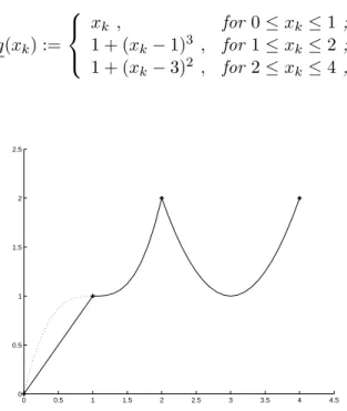
3.1 A piecewise-defined univariate function . . . 34

3.2 A piecewise-convex lower approximation . . . 34

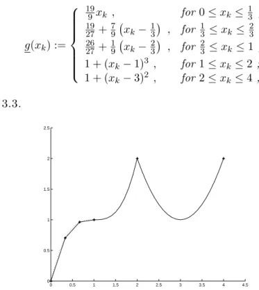
3.3 An improved piecewise-convex lower approximation . . . 35

3.4 The convex relaxation . . . 37

3.5 The algorithmic framework . . . 39

3.6 UFL: how−gkt(wkt) looks like in the three instances. . . 41

3.7 Hydro UC: how−ϕ(qjt) looks like in the three instances . . . 42

4.1 Piecewise linear approximation of a univariate function, and its adaptation to a function of two variables. . . 46

4.2 Geometric representation of the triangle method. . . 49

4.3 Geometric representation of the triangle method. . . 50

4.4 Five functions used to evaluate the approximation quality. . . 52

5.1 Examples off(x) for (a) binary and (b) general integer variables. . . 58

5.2 sp 6-sp 9 are the combination of solutions (1.4, 1.2) and (3.2, 3.7) represented by one point of the line linking the two points. . . 63

5.3 An ideal cut should make the range [0.5,0.8] infeasible. . . 65

5.4 N LPf can have lots of local minima. . . 66

6.1 The simple approximation . . . 74

6.2 The enhanced approximation . . . 77

6.3 Piecewise approximation of the relationship (6.19) for three volume values . . 79

6.4 Water volumes . . . 83

6.5 Inflow and flows . . . 85

6.6 Price and powers . . . 85

6.7 Profit . . . 86

7.1 Three polynomials of different degree approximating the cost function for in-stancefoss poly 0, see Section 7.5.1. . . 91

(12)

7.2 Smoothingf near x= 0. . . 93 7.3 Solution for Fossolo network, version foss iron. . . 104

(13)

List of Tables

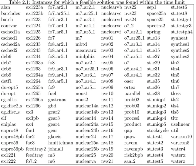
2.1 Instances for which a feasible solution was found within the time limit . . . . 28

2.2 Instances for which the feasible solution found is also the best-know solution 29 2.3 Instances for which no feasible solution was found within the time limit . . . 29

2.4 Instances with problems during the execution . . . 29

3.1 Results for Uncapacitated Facility Location problem . . . 41

3.2 Results for Hydro Unit Commitment and Scheduling problem . . . 42

3.3 Results for GLOBALLib and MINLPLib . . . 44

4.1 Average approximation quality for different values ofn,m,x and y. . . 52

4.2 Comparison with respect to the size of the MILP. . . 55

4.3 MILP results with different time limits expressed in CPU seconds. . . 55

5.1 Comparison among different NLP solvers used for solving problemN LPf. . . 62

5.2 Results using different starting points. . . 64

5.3 Instancegesa2-o . . . 65

5.4 Instancevpm2 . . . 65

6.1 Results for a turbine with theϕ1 characteristic of Figure 6.3 . . . 80

6.2 Results for a turbine with theϕ2 characteristic of Figure 6.3 . . . 80

6.3 Number of variables and constraints for the three models considering 8 config-urations of (t;r;z) . . . 82

6.4 Results with more volume intervals for April T168 and a turbine with the characteristic of Figure 6.3 . . . 82

6.5 Results for BDLM+ with and without the BDLM solution enforced . . . 83

6.6 Results for the MILP model with 7 volume intervals and 5 breakpoints . . . . 84

7.1 Water Networks. . . 97

7.2 Characteristics of the 50 continuous solutions at the root node. . . 101

7.3 Computational results for the MINLP model (part 1). Time limit 7200 seconds.102 7.4 Computational results for the MINLP model (part 2). Time limit 7200 seconds. 102 7.5 Computational results for the MINLP model comparing the fitted and the discrete objective functions. Time limit 7200 seconds. . . 103

7.6 MINLP results compared with literature results. . . 106

8.1 Convex instances of MINLPlib (info heuristically computed with LaGO). . . 130 8.2 Non-convex instances of MINLPlib (info heuristically computed with LaGO). 130

(14)

(15)

Preface

In the most recent years there is a renovate interest for Mixed Integer Non-Linear Program-ming (MINLP) problems. This can be explained for different reasons: (i) the performance of solvers handling non-linear constraints was largely improved; (ii) the awareness that most of the applications from the real-world can be modeled as an MINLP problem; (iii) the challeng-ing nature of this very general class of problems. It is well-known that MINLP problems are NP-hard because they are the generalization of MILP problems, which are NP-hard them-selves. This means that it is very unlikely that a polynomial-time algorithm exists for these problems (unless P = NP). However, MINLPs are, in general, also hard to solve in prac-tice. We address to non-convex MINLPs, i.e. having non-convex continuous relaxations: the presence of non-convexities in the model makes these problems usually even harder to solve. Until recent years, the standard approach for handling MINLP problems has basically been solving an MILP approximation of it. In particular, linearization of the non-linear constraints can be applied. The optimal solution of the MILP might be neither optimal nor feasible for the original problem, if no assumptions are done on the MINLPs. Another possible approach, if one does not need a proven global optimum, is applying the algorithms tailored for convex MINLPs which can be heuristically used for solving non-convex MINLPs. The third approach to handle non-convexities is, if possible, to reformulate the problem in order to obtain a special case of MINLP problems. The exact reformulation can be applied only for limited cases of non-convex MINLPs and allows to obtain an equivalent linear/convex formulation of the convex MINLP. The last approach, involving a larger subset of non-convex MINLPs, is based on the use of non-convex envelopes or underestimators of the non-non-convex feasible region. This allows to have a lower bound on the non-convex MINLP optimum that can be used within an algorithm like the widely used Branch-and-Bound specialized versions for Global Optimization. It is clear that, due to the intrinsic complexity from both practical and theoretical viewpoint, these algorithms are usually suitable at solving small to medium size problems.

The aim of this Ph.D. thesis is to give a flavor of different possible approaches that one can study to attack MINLP problems with non-convexities, with a special attention to real-world problems. In Part I of the thesis we introduce the problem and present three special cases of general MINLPs and the most common methods used to solve them. These techniques play a fundamental role in the resolution of general MINLP problems. Then we describe algorithms addressing general MINLPs. Parts II and III contain the main contributions of the Ph.D. thesis. In particular, in Part II four different methods aimed at solving different classes of MINLP problems are presented. More precisely:

In Chapter 2 we present a Feasibility Pump (FP) algorithm tailored for non-convex

Mixed Integer Non-Linear Programming problems. Differences with the previously pro-xiii

(16)

posed FP algorithms and difficulties arising from non-convexities in the models are extensively discussed. We show that the algorithm behaves very well with general prob-lems presenting computational results on instances taken from MINLPLib.

In Chapter 3 we focus on separable non-convex MINLPs, that is where the objective

and constraint functions are sums of univariate functions. There are many problems that are already in such a form, or can be brought into such a form via some simple substitutions. We have developed a simple algorithm, implemented at the level of a modeling language (in our case AMPL), to attack such separable problems. First, we identify subintervals of convexity and concavity for the univariate functions using external calls to MATLAB. With such an identification at hand, we develop a convex MINLP relaxation of the problem. We work on each subinterval of convexity and concavity separately, using linear relaxation on only the “concave side” of each function on the subintervals. The subintervals are glued together using binary variables. Next, we repeatedly refine our convex MINLP relaxation by modifying it at the modeling level. Next, by fixing the integer variables in the original non-convex MINLP, and then locally solving the associated non-convex NLP relaxation, we get an upper bound on the global minimum. We present preliminary computational experiments on different instances.

In Chapter 4 we consider three methods for the piecewise linear approximation of

functions of two variables for inclusion within MILP models. The simplest one applies the classical one-variable technique over a discretized set of values of the second inde-pendent variable. A more complex approach is based on the definition of triangles in the three-dimensional space. The third method we describe can be seen as an intermediate approach, recently used within an applied context, which appears particularly suitable for MILP modeling. We show that the three approaches do not dominate each other, and give a detailed description of how they can be embedded in a MILP model. Advan-tages and drawbacks of the three methods are discussed on the basis of some numerical examples.

In Chapter 5 we present preliminary computational results on heuristics for Mixed

Integer Linear Programming. A heuristic for hard MILP problems based on NLP tech-niques is presented: the peculiarity of our approach to MILP problems is that we re-formulate integrality requirements treating them in the non-convex objective function, ending up with a mapping from the MILP feasibility problem to NLP problem(s). For each of these methods, the basic idea and computational results are presented.

Part III of the thesis is devoted to real-world applications: two different problems and ap-proaches to MINLPs are presented, namely Scheduling and Unit Commitment for Hydro-Plants and Water Network Design problems. The results show that each of these different methods has advantages and disadvantages. Thus, typically the method to be adopted to solve a real-world problem should be tailored on the characteristics, structure and size of the problem. In particular:

Chapter 6deals with a unit commitment problem of a generation company whose aim

is to find the optimal scheduling of a multi-unit pump-storage hydro power station, for a short term period in which the electricity prices are forecasted. The problem has a mixed-integer non-linear structure, that makes very hard to handle the corresponding

(17)

xv mathematical models. However, modern MILP software tools have reached a high ef-ficiency, both in terms of solution accuracy and computing time. Hence we introduce MILP models of increasing complexity, that allow to accurately represent most of the hydro-electric system characteristics, and turn out to be computationally solvable. In particular, we present a model that takes into account the head effects on power pro-duction through an enhanced linearization technique, and turns out to be more general and efficient than those available in the literature. The practical behavior of the models is analyzed through computational experiments on real-world data.

In Chapter 7we present a solution method for a water-network optimization problem using a non-convex continuous NLP relaxation and a MINLP search. Our approach employs a relatively simple and accurate model that pays some attention to the re-quirements of the solvers that we employ. Our view is that in doing so, with the goal of calculating only good feasible solutions, complicated algorithmics can be confined to the MINLP solver. We report successful computational experience using available open-source MINLP software on problems from the literature and on difficult real-world instances.

Part IV of the thesis consists of a brief review on tools commonly used for general MINLP problems. We present the main characteristics of solvers for each special case of MINLP. Then we present solvers for general MINLPs: for each solver a brief description, taken from the manuals, is given together with a schematic table containing the most importart pieces of information, for example, the class of problems they address, the algorithms implemented, the dependencies with external software.

Tools for MINLP, especially open-source software, constituted an integral part of the development of this Ph.D. thesis. Also for this reason Part IV is devoted to this topic. Methods presented in Chapters 4, 5 and 7 were completely developed using open-source solvers (and partially Chapter 3). A notable example of the importance of open-source solvers is given in Chapter 7: we present an algorithm for solving a non-convex MINLP problem, namely the Water Network Design problem, using the open-source software Bonmin. The solver was originally tailored for convex MINLPs. However, some accommodations were made to handle non-convex problems and they were developed and tested in the context of the work presented in Chapter 7, where details on these features can be found.

(18)

(19)

Part I

Introduction

(20)

(21)

Chapter 1

Introduction to Mixed Integer

Non-Linear Programming Problems

and Methods

The (general) Mixed Integer Non-Linear Programming (MINLP) problem which we are in-terested in has the following form:

MINLP

minf(x, y) (1.1)

g(x, y) ≤ 0 (1.2)

x ∈ X∩Zn (1.3)

y ∈ Y , (1.4)

wheref :Rn×p →R,g:Rn×p →Rm,X and Y are two polyhedra of appropriate dimension (including bounds on the variables). We assume thatf and g are twice continuously differ-entiable, but we do not make any other assumption on the characteristics of these functions or their convexity/concavity. In the following, we will call problems of this type non-convex Mixed Integer Non-Linear Programming problems.

Non-convex MINLP problems are NP-hard because they generalize MILP problems which are NP-hard themselves (for a detailed discussion on the complexity of MILPs we refer the reader to Garey and Johnson [61]).

The most complex aspect we need to have in mind when we work with non-convex MINLPs is that its continuous relaxation, i.e. the problem obtained by relaxing the integrality require-ment on the x variables, might have (and usually it has) local optima, i.e. solutions which are optimal within a restricted part of the feasible region (neighborhood), but not considering the entire feasible region. This does not happen whenf andgare convex (or linear): in these cases the local optima are also global optima, i.e. solutions which are optimal considering the entire feasible region.

To understand more in detail the issue, let us consider the continuous relaxation of the MINLP problem. The first order optimality conditions are necessary, but, only whenf and

gare convex, they are also sufficient for the stationary point (x, y) which satisfies them to be 3

(22)

the global optimum: g(x, y) ≤ 0 (1.5) x ∈ X (1.6) y ∈ Y (1.7) λ ≥ 0 (1.8) ∇f(x, y) + m X i=1 λi∇gi(x, y) = 0 (1.9) λTg(x, y) = 0, (1.10)

where∇is the Jacobian of the function andλare the dual variables, i.e. the variables of the Dual problem of the continuous relaxation of MINLP which is called Primal problem. The Dual problem is formalized as follows:

max

λ≥0[infx∈X,y∈Yf(x, y) +λ

T_g₍_{x, y}_)]_, _(1.11)

see [17, 97] for details on Duality Theory in NLP. Equations (1.5)-(1.7) are the primal feasibil-ity conditions, equation (1.8) is the dual feasibilfeasibil-ity condition, equation (1.9) is the stationarfeasibil-ity condition and equation (1.10) is the complementarity condition.

These conditions, called also Karush-Kuhn-Tucker (KKT) conditions, assume an impor-tant role in algorithms we will present and use in this Ph.D. thesis. For details the reader is referred to Karush [74], Kuhn and Tucker [77].

The aim of this Ph.D. thesis is presenting methods for solving non-convex MINLPs and models for real-world applications of this type. However, in the remaining part of this sec-tion, we will present special cases of general MINLP problems because they play an important role in the resolution of the more general problem. Though, this introduction will not cover exhaustively topics concerning Mixed Integer Linear Programming (MILP), Non-Linear Pro-gramming (NLP) and Mixed Integer Non-Linear ProPro-gramming in general, but only give a flavor of the ingredients necessary to fully understand the methods and algorithms which are the contribution of the thesis. For each problem, references will be provided to the interested reader.

1.1 Mixed Integer Linear Programming

A Mixed Integer Linear Programming problem is the special case of the MINLP problem in which functions f and g assume a linear form. It is usually written in the form:

MILP

mincTx+dTy

Ax+By ≤ b

x ∈ X∩Zn

y ∈ Y,

whereA and B are, respectively, them×nand the m×p matrices of coefficients, b is the

(23)

1.1. MIXED INTEGER LINEAR PROGRAMMING 5 thep-dimensional vectors of costs. Even if these problems are a special and, in general, easier case with respect to MINLPs, they are NP-hard (see Garey and Johnson [61]). This means that a polynomial algorithm to solve MILP is unlikely to exists, unless P = NP.

Different possible approaches to this problem have been proposed. The most effective ones and extensively used in the modern solvers are Branch-and-Bound (see Land and Doig [78]), cutting planes (see Gomory [64]) and Branch-and-Cut (see Padberg and Rinaldi [102]). These are exact methods: this means that, if an optimal solution for the MILP problem exists, they find it. Otherwise, they prove that such a solution does not exist. In the following we give a brief description of the main ideas of these methods, which, as we will see, are the basis for the algorithms proposed for general MINLPs.

Branch-and-Bound(BB): the first step is solving the continuous relaxation of MILP (i.e. the problem obtained relaxing the integrality constraints on thex variables, LP =

{mincT_x₊_dT_y _|_Ax₊_By_≤_{b, x}_∈_{X, y}_∈_Y_}_{). Then, given a fractional value}_x∗

j from the solution of LP (x∗_{, y}∗_{), the problem is divided into two subproblems, the first where}

the constraint xj ≤ ⌊x∗j⌋ is added and the second where the constraint xj ≥ ⌊x∗j⌋+ 1 is added. Each of these new constraints represents a “branching decision” because the partition of the problem in subproblems is represented with a tree structure, the BB tree. Each subproblem is represented as a node of the BB tree and, from a mathematical viewpoint, has the form:

LP _min_cT_x₊_dT_y Ax+By ≤ b x ∈ X y ∈ Y x ≤ lk x ≥ uk,

where lk _and _uk _{are vectors defined so as to mathematically represent the branching} decisions taken so far in the previous levels of the BB tree. The process is iterated for each node until the solution of the continuous relaxation of the subproblem is integer feasible or the continuous relaxation is infeasible or the lower bound value of subprob-lem is not smaller than the current incumbent solution, i.e. the best feasible solution encountered so far. In these three cases, the node is fathomed. The algorithm stops when no node to explore is left, returning the best solution found so far which is proven to be optimal.

Cutting Plane(CP): as in the Branch-and-Bound method, the LP relaxation is solved. Given the fractional LP solution (x∗_{, y}∗_{), a separation problem is solved, i.e. a problem}

whose aim is finding a valid linear inequality that cuts off (x∗_{, y}∗_{), i.e. it is not satisfied}

by (x∗, y∗). An inequality is valid for the MILP problem if it is satisfied by any integer feasible solution of the problem. Once a valid inequality (cut) is found, it is added to the problem: it makes the LP relaxation tighter and the iterative addition of cuts might lead to an integer solution. Different types of cuts have been studied, for example, Gomory mixed integer cuts, Chv´atal-Gomory cuts, mixed integer rounding cuts, rounding cuts, lift-and-project cuts, split cuts, clique cuts (see [40]). Their effectiveness depends on the MILP problem and usually different types of cuts are combined.

(24)

Branch-and-Cut(BC): the idea is integrating the two methods described above, merg-ing the advantages of both techniques. Like in BB, at the root node the LP relaxation is solved. If the solution is not integer feasible, a separation problem is solved and, in the case cuts are fonud, they are added to the problem, otherwise a branching decision is performed. This happens also to non-leaf nodes, the LP relaxation correspondent to the node is solved, a separation problem is computed and cuts are added or branch is performed. This method is very effective and, like in CP, different types of cuts can be used.

An important part of the modern solvers, usually integrated with the exact methods, are heuristic methods: their aim is finding rapidly a “good” feasible solution or improving the best solution found so far. No guarantee on the optimality of the solution found is given. Examples of the first class of heuristics are: simple rounding heuristics, Feasibility Pump (see Fischetti et al. [50], Bertacco et al. [16], Achterberg and Berthold [3]). Examples of the second class of heuristics are metaheuristics (see, for example, Glover and Kochenberger [63]), Relaxation Induced Neighborhoods Search (see Danna et al. [43]) and Local Branching (see Fischetti and Lodi [51]).

For a survey of the methods and the development of the software addressed at solving MILPs the reader is referred to the recent paper by Lodi [87], and for a detailed discussion see [2, 18, 19, 66, 95, 104].

1.2 Non-Linear Programming

Another special case of MINLP problems is Non-Linear Programming: the functionsf and g

are non-linear butn= 0, i.e. no variable is required to be integer. The classical NLP problem can be written in the following form:

NLP

minf(y) (1.12)

g(y) ≤ 0 (1.13)

y ∈ Y. (1.14)

Different issues arise when one tries to solve this kind of problems. Some heuristic and exact methods are tailored for a widely studied subclass of these problems: convex NLPs. In this case, the additional assumption is that f and g are convex functions. Some of these methods can be used for more general non-convex NLPs, but no guarantee on the global optimality of the solution is given. In particular, when no assumption on convexity is done, the problem usually has local optimal solutions. In the non-convex case, exact algorithms, i.e. those methods that are guaranteed to find the global solution, are called Global Optimization methods.

In the following we sketch some of the most effective algorithms studied and actually implemented within available NLP solvers (see Section 8):

Line Search: introduced for unconstrained optimization problems with non-linear ob-jective function, it is an iterative method used also as part of methods for constrained NLPs. At each iteration an approximation of the non-linear function is considered and (i) a search direction is decided; (ii) the step length to take along that direction is

(25)

1.2. NON-LINEAR PROGRAMMING 7 computed and (iii) the step is taken. Different approaches to decide the direction and the step length are possible (e.g., Steepest descent, Newton, Quasi-Newton, Conjugate Direction methods).

Trust Region: it is a method introduced as an alternative to Line Search. At each iteration, the search of the best point using the approximation is limited into a “trust region”, defined with a maximum step length. This approach is motivated by the fact that the approximation of the non-linear function at a given point can be not good far away from that point, then the “trust region” represents the region in which we suppose the approximation is good. Then the direction and the step length which allow the best improvement of the objective function value within the trust region is taken. (The size of the trust region can vary depending on the improvements obtained at the previous iteration.) Also in this case different possible strategies to choose the direction and the step length can be adopted.

Active Set: it is an iterative method for solving NLPs with inequalities. The first step of each iteration is the definition of the active set of constraints, i.e. the inequalities which are strictly satisfied. Considering the surface defined by the constraints within the active set, a move on the surface is decided, identifying the new point for the next iteration. The Simplex algorithm by Dantzig [44] is an Active Set method for solving Linear Programming problems. An effective and widely used special case of Active Set method for NLPs is the Sequential Quadratic Programming (SQP) method. It solves a sequence of Quadratic Programming (QP) problems which approximate the NLP problem at the current point. An example of such an approximation is using the Newton’s method to the KKT conditions of the NLP problem. The QP problems are solved using specialized QP solvers.

Interior Point: in contrast to the Active Set methods which at each iteration stay on a surface of the feasible region, the Interior Point methods stay in the strict interior of it. From a mathematical viewpoint, at each iteration, conditions of primal and dual feasibility (1.5)-(1.8) are satisfied and complementarity conditions (1.10) are relaxed. The algorithm aims at reducing the infeasibility of the complementarity constraints.

Penalty and Augmented Lagrangian: it is a method in which the objective function

of NLP is redefined in order to take into account both the optimality and the feasibility of a solution adding a term which penalizes infeasible solutions. An example of a Penalty method is the Barrier algorithm which uses an interior type penalty function. When a penalty function is minimized at the solution of the original NLP, it is called exact, i.e. the minimization of the penalty function leads to the optimal solution of the original NLP problem. An example of exact Penalty method is the Augmented Lagrangian method, which makes explicit use of the Lagrange multiplier estimates.

Filter: it is a method in which the two goals (usually competing) which in Penalty methods are casted within the same objective function, i.e. optimality and feasibility, are treated separately. So, a point can become the new iterate point only if it is not dominated by a previous point in terms of optimality and feasibility (concept closely related to Pareto optimality).

(26)

For details on the algorithms mentioned above and their convergence, the reader is referred to, for example, [12, 17, 29, 54, 97, 105]. In the context of the contribution of this Ph.D. thesis, the NLP methods and solvers are used as black boxed, i.e. selecting them according to their characteristics and efficiency with respect to the problem, but without changing them.

1.3 Convex Mixed Integer Non-Linear Programming

The third interesting subclass of general MINLP is the convex MINLP. The form of these problems is the same as MINLP, butf and gare convex functions. The immediate and most important consideration derived by this assumption is that each local minimum of the problem is guaranteed to be also a global minimum of the continuous relaxation. This property is exploited in methods studied specifically for this class of problems. In the following we briefly present the most used approaches to solve convex MINLPs, in order to have an idea of the state of the art regarding solution methods of MINLP with convexity properties. Because the general idea of these methods is solving “easier” subproblems of convex MINLPs, we first define three different important subproblems which play a fundamental role in the algorithms we are going to describe.

M ILPk minz f(xk, yk) +∇f(xk, yk)T x−xk y−yk ≤z g(xk_{, y}k_{) +}_∇g₍_xk_{, y}k₎T x−xk y−yk ≤0        k= 1, . . . , K x∈X∩Zn y ∈Y,

where z is an auxiliary variable added in order to have a linear objective function, (xk_{, y}k_{) refers to a specific value of} _x_and _y_{. The original constraint are substituted by} their linearization constraints called Outer Approximation cuts.

N LPk minf(x, y) g(x, y) ≤ 0 x ∈ X y ∈ Y x ≤ lk x ≥ uk,

where lk _and _uk _{are, respectively, the lower and upper bound on the integer variables} specific of subproblem N LPk_{. This is the continuous subproblem corresponding to} a specific node of the Branch-and-Bound tree, i.e. the NLP version of LPk. If no branching decision has been taken on a specific variable, say xj, lj is equal to −∞ and uj is equal to +∞ (i.e. the original bounds, included in x ∈ X, are preserved). Otherwise,lk

(27)

1.3. CONVEX MIXED INTEGER NON-LINEAR PROGRAMMING 9

N LPk_x

minf(xk, y)

g(xk, y) ≤ 0

y ∈ Y,

where the integer part of the problem is fixed according to the integer vector xk_. Algorithms studied for convex MINLPs differ basically on how the subproblems involved are defined and used. We present briefly some of the most used algorithms and refer the reader to the exhaustive paper by Grossmann [65].

Branch-and-Bound (BB): the method, originally proposed for MILP problems (see

Section 1.1), was adapted for general convex MINLPs by Gupta and Ravindran [70]. The basic difference is that, at each node, an LP subproblem is solved in the first case, an NLP subproblem in the second. We do not discuss specific approaches for branching variable selection, tree exploration strategy, etc. For details the reader is referred to [1, 20, 70, 82].

Outer-Approximation (OA): proposed by Duran and Grossman [45], it exploits the

Outer Approximation linearization technique which is “safe” for convex functions, i.e. it does not cut off any solution of the MINLP. It is an iterative method in which, at each iteration k, a N LPk_x and a M ILPk subproblem are solved (the vector xk _{used in}

N LPk

x is taken from the solution of M ILPk). The first subproblem, if feasible, gives an upper bound on the solution of the MINLP and the second subproblem always gives a lower bound. At each iteration the lower and the upper bounds might be improved, in particular the definition of M ILPk _{changes because, at each iteration, OA cuts are} added which cut off the solution of the previous iteration. The algorithm ends when the two bounds assume the same value (within a fixed tolerance).

Generalized Benders Decomposition (GBD): like BB, it was first introduced for

MILPs (see Benders [15]). Geoffrion [62] adapted the method to convex MINLP prob-lems. It is strongly related to the OA method, the unique difference being the form of theM ILPk subproblem. TheM ILPk of the GBD method is a surrogate relaxation of the one of the OA method and the lower bound given by the OA M ILPk _{is stronger} than (i.e. greater or equal to) the one given by the GBDM ILPk(for details, see Duran and Grossmann [45]). More precisely, the GBD M ILPk constraints are derived from the OA constraints generated only for the active inequalities ({i|gi(xk, yk) = 0}) plus the use of KKT conditions and projection in thex-space:

f(xk, yk) +∇xf(xk, yk)T(x−xk) + (µk)[g(xk, yk) +∇xg(xk, yk)T(x−xk)]≤z where µk _{is the vector of dual variables corresponding to original constraints (1.2) (see} [65] for details this relationship). These Lagrangian cuts projected in the x-space are weaker, but the GBDM ILPk is easier to solve with respect to the OAM ILPk. Even if, on average, the number of iterations necessary for the GBD method is bigger than the one for the OA method, the tradeoff among number of iterations and computational effort of each iteration makes sometimes convenient using one or the other approach.

(28)

Extended Cutting Plane (ECP): introduced by Westerlund and Pettersson [126], the method is based on the iterative resolution of aM ILPk subproblem and, given the optimal solution of M ILPk _{which can be infeasible for}_{M IN LP}_{, the determination of} the most violated constraint (or more), whose linearization is added at the nextM ILPk. The given lower bound is decreased at each iteration, but generally a large number of iterations is needed to reach the optimal solution.

LP/NLP based Branch-and-Bound(QG): the method can be seen as the extention

of the Branch-and-Cut to convex MINLPs (see Quesada and Grossmann [108]). The idea is solving with BB the M ILPk 1 _{subproblem not multiple times but only once.}

This is possible if, at each node at which an integer feasible solution is found, theN LPkx subproblem is solved, OA cuts are then generated and added to theM ILPkof the open nodes of the Branch-and-Bound tree.

Hybrid algorithm (Hyb): an enhanced version of QG algorithm was recently

devel-oped by Bonami et al. [20]. It is called Hybrid algorithm because it combines BB and OA methods. In particular, the differences with respect to the QG algorithm are that at “some” nodes (not only when an integer solution is found) theN LPk_x subproblem is solved to generate new cuts (like in BB) and local enumerations at some nodes of the tree are performed (it can be seen as performing some iterations of the OA algorithm at some nodes). When the local enumeration is not limited, the Hyb algorithm reconduces to OA, when the N LPk_x is solved at each node, it reconduces to BB.

As for MILP solvers, heuristic algorithms also play an important role within MINLP solvers. Part of the heuristic algorithms studied for MILPs have been adapted for convex MINLP problems. For details about primal heuristics the reader is referred to, for example, [1, 21, 23].

Specific algorithms have been also studied for special cases of convex MINLPs (see, e.g., [56, 69, 109]). Methods which exploit the special structure of the problem are usually much more efficient than general approaches.

1.4 Non-convex Mixed Integer Non-Linear Programming

Coming back to the first model seen in this chapter, MINLP, we do not have any convexity assumption on the objective function and the constraints. As discussed, one of the main issues regarding non-convex MINLP problems is that there are, in general, local minima which are not global minima. This issue implies, for example, that, if the NLP solver used to solve

N LPk _and _{N LP}k

x subproblems does not guarantee that the solution provided is a global optimum (and this is usually the case for the most common NLP solvers, see Chapter 8), feasible and even optimal solutions might be cut off if methods like BB, QG and Hyb of Section 1.4 are used. This happens, for example, when a node is fathomed because of the lower bound (the value of a local minimum can be much worse than the one of the global minimum). This makes these methods, that are exact for convex MINLPs, heuristics for non-convex MINLPs. A second issue involves methods OA, GBD, ECP, QG and Hyb of Section 1.4: the linearization cuts used in these methods are in general not valid for non-convex

1_The_{M ILP}k_{definition is obtained using the solution (}_x0_{, y}0_{) of}_{N LP}k_{solved just once for the initialization}

(29)

1.4. NON-CONVEX MIXED INTEGER NON-LINEAR PROGRAMMING 11 constraints. It means that the linearization cuts might cut off not only infeasible points, but also parts of the feasible region (see Figure 1.1). For this reason, when non-convex constraints are involved, one has to carefully use linearization cuts.

0 1 2 3 4 5 6 −20 −15 −10 −5 0 5 10 15 20

Figure 1.1: Example of “unsafe” linearization cut generated from a non-convex constraint The first approach to handle non-convexities is, if possible, to reformulate the problem. The exact reformulation can be applied only for limited cases of non-convex MINLPs and allows to obtain an equivalent convex formulation of the non-convex MINLP. All the tech-niques described in Section 1.3 can then be applied to the reformulated MINLP. For a detailed description of exact reformulations to standard forms, see, for example, Liberti’s Ph.D. thesis [83].

The second approach, involving a larger subset of non-convex MINLPs, is based on the use of convex envelopes or underestimators of the non-convex feasible region. This allows to have a lower bound on the non-convex MINLP optimum that can be used within an algorithm like the widely used Branch-and-Bound specialized versions for Global Optimization, e.g., spatial Branch-and-Bound (see [118, 81, 83, 14]), Branch-and-Reduce (see [110, 111, 119]),α-BB (see [6, 5]), Branch-and-Cut (see [76, 100]). The relaxation of the original problem, obtained using convex envelopes or underestimators of the non-convex functions, rMINLP has the form:

minz (1.15)

f(x, y) ≤ z (1.16)

g(x, y) ≤ 0 (1.17)

x ∈ X∩Zn (1.18)

y ∈ Y, (1.19)

(30)

R and g:Rn×p →Rm are convex (in some cases, linear) functions andf(x, y)≤f(x, y) and

g(x, y)≤g(x, y) within the (x, y) domain.

Explanations on different ways to define functionsf(x, y) andg(x, y) for non-convex func-tionsf andg with specific structure can be found, for example, in [83, 92, 98]. Note anyway that, in general, these techniques apply only for factorable functions, i.e. function which can be expressed as summations and products of univariate functions, which can be reduced and reformulated as predetermined operators for which convex underestimators are known, such as, for example, bilinear, trilinear, fractional terms (see [84, 92, 118]).

The use of underestimators makes the feasible region larger; if the optimal solution of rMINLP is feasible for the non-convex MINLP, then it is also its global optimum. Otherwise, i.e. if the solution of rMINLP is infeasible for MINLP, a refining on the underestimation of the non-convex functions is needed. This is done by branching, not restricted to integer variables but also on continuous ones (see Figure 1.2).

0 1 2 3 4 5 6 −20 −15 −10 −5 0 5 10 15 20 0 1 2 3 4 5 6 −20 −15 −10 −5 0 5 10 15 20

Figure 1.2: Linear underestimators before and after branching on continuous variables The specialized Branch-and-Bound methods for Global Optimization we mentioned before mainly differ on the branching scheme adopted: (i) branch both on continuous and discrete variables without a prefixed priority; (ii) branch on continuous variables and apply standard techniques for convex MINLPs at each node; (ii) branch on discrete variables until an integer feasible solution is found, then branch on continuous variables.

It is clear that an algorithm of this type is very time-expensive in general. This is the price one has to pay for the guarantee of the global optimality of the solution provided (within a fixed tolerance). Moreover, from an implementation viewpoint, some complex structures are needed. For example, it is necessary to describe the model with symbolic mathematical expressions which is important if the methods rely on tools for the symbolic and/or automatic differentiation. Moreover, in this way it is possible to recognize factors, structures and refor-mulate the components of the model so as one needs to deal only with standard operators which can be underestimated with well-known techniques. These and other complications arising in the non-convex MINLP software will be discussed more in detail in Chapter 8.

If one does not need a proven global optimum, the algorithms presented in Section 1.3 can be (heuristically) used for solving non-convex MINLPs, i.e. by ignoring the problems explained at the beginning of this section. One example of application of convex methods to non-convex MINLP problems will be presented in Chapter 7. The BB algorithm of the convex

(31)

1.5. GENERAL CONSIDERATIONS ON MINLPS 13 MINLP solver Bonmin [26], modified to limit the effects of non-convexities, was used. Some of these modifications were implemented in Bonmin while studying the application described in Chapter 7 and are now part of the current release.

Also in this case, heuristics studied originally for MILPs have been adapted for non-convex MINLPs. An example is given by a recent work of Liberti et al. [86]. In Chapter 2 we will present a new heuristic algorithm extending to non-convex MINLPs the Feasibility Pump (FP) heuristic ideas for MILPs and convex MINLPs. Using some of the basic ideas of the original FP for solving non-convex MINLPs is not possible for the same reasons we explained before. Also in this case algorithms studied for convex MINLPs encounter problems when applied to non-convex MINLPs. In Chapter 2 we will explain in detail how we can limit these difficulties.

Specific algorithms have been also studied for special cases of non-convex MINLPs (see, e.g., [73, 107, 113]). As for convex MINLPs, methods which exploit the special structure of the problem are usually much more efficient than general approaches. Examples are given in Chapters 3.

1.5 General considerations on MINLPs

Until recent years, the standard approach for handling MINLP problems has basically been solving an MILP approximation of it. In particular, linearization of the non-linear constraints can be applied. Note, however, that this approach differs from, e.g., OA, GBD and ECP presented in Section 1.3 because the linearization is decided before the optimization starts, the definition of the MILP problem is never modified and no NLP (sub)problem resolution is performed. This allows using all the techniques described in Section 1.1, which are in general much more efficient than the methods studied for MINLPs. The optimal solution of the MILP might be neither optimal nor feasible for the original problem, if no assumptions are done of the MINLPs. If, for example, f(x, y) is approximated with a linear objective function, say f(x, y), and g(x, y) with linear functions, say g(x, y), such that f(x, y) ≥ f(x, y) and

g(x, y) ≥ g(x, y), the MILP approximation provide a lower bound on the original problem. Note that, also in this case, the optimum of the MILP problem is not guaranteed to be feasible for the original MINLP, but, in case it is feasible for the MINLP problem, we have the guarantee that it is also the global optimum.

In Chapter 4, a method for approximating non-linear functions of two variables is pre-sented: comparisons to the more classical methods like piecewise linear approximation and triangulation are reported. In Chapter 6 we show an example of application in which applying these techniques is successful. We will show when it is convenient applying MINLP techniques in Chapter 7.

Finally, note that the integrality constraint present in Mixed Integer Programming prob-lems can be seen as a source of non-convexity for the problem: it is possible to map the feasibility problem of an MILP problem into an NLP problem. Due to this consideration, we studied NLP-based heuristics for MILP problems: these ideas are presented in Chapter 5.

(32)

(33)

Part II

Modeling and Solving

Non-Convexities

(34)

(35)

Chapter 2

A Feasibility Pump Heuristic for

Non-Convex MINLPs

1

2.1 Introduction

Heuristic algorithms have always played a fundamental role in optimization, both as inde-pendent tools and as part of general-purpose solvers. Starting from Mixed Integer Linear Programming (MILP), different kinds of heuristics have been proposed: their aim is finding a good feasible solution rapidly or improving the best solution found so far. Within a MILP solver context, both types of heuristics are used. Examples of heuristic algorithms are round-ing heuristics, metaheuristics (see, e.g., [63]), Feasibility Pump [50, 16, 3], Local Branchround-ing [51] and Relaxation Induced Neighborhoods Search [43]. Even if the heuristic algorithms might find the optimal solution, no guarantee on the optimality is given.

In the most recent years Mixed Integer Non-Linear Programming (MINLP) has become a topic capable of attracting the interest of the research community. This is due from the one side to the continuous improvements of Non-Linear Programming (NLP) solvers and on the other hand to the wide range of real-world applications involving these problems. A special focus has been devoted to convex MINLPs, a class of MINLP problems whose nice properties can be exploited. In particular, under the convexity assumption, any local optimum is also a global optimum of the continuous relaxation and the use of standard linearization cuts like Outer Approximation (OA) cuts [45] is possible, i.e. the generated cuts are valid. Heuristics have been proposed recently also for this class of problems. Basically the ideas originally tailored on MILP problems have been extended to convex MINLPs, for example, Feasibility Pump [21, 1, 23] and diving heuristics [23].

The focus of this chapter is proposing a heuristic algorithm for non-convex MINLPs. These problems are in general very difficult to solve to optimality and, usually, like sometimes also happens for MILP problems, finding any feasible solution is also a very difficult task in practice (besides being NP-hard in theory). For this reason, heuristic algorithms assume a fundamental part of the solving phase. Heuristic algorithms proposed so far for non-convex MINLPs are, for example, Variable Neighborhood Search [86] and Local Branching [93], but

1_{This is a working paper with Antonio Frangioni (DI, University of Pisa), Leo Liberti (LIX, Ecole} Poly-technique) and Andrea Lodi (DEIS, University of Bologna).

(36)

this field is still highly unexplored. This is mainly due to the difficulties arising from the lack of structures and properties to be exploited for such a general class of problems.

We already mentioned the innovative approach to the feasibility problem for MILPs, called Feasibility Pump, which was introduced by Fischetti et al. [50] for problems with integer vari-ables restricted to be binary and lately extended to general integer by Bertacco et al. [16]. The idea is to iteratively solve subproblems of the original difficult problem with the aim of “pumping” the feasibility in the solution. More precisely, Feasibility Pump solves the conti-nous relaxation of the problem trying to minimize the distance to an integer solution, then rounding the fractional solution obtained. Few years later a similar technique applied to con-vex MINLPs was proposed by Bonami et al. [21]. In this case, at each iteration, an NLP and an MILP subproblems are solved. The authors also prove the convergence of the algorithm and extend the same result to MINLP problems with non-convex constraints, defining, how-ever, a convex feasible region. More recently Bonami and Goncalves [23] proposed a less time consuming version in which the MILP resolution is substituted by a rounding phase similar to that originally proposed by Fischetti et al. [50] for MILPs.

In this chapter, we propose a Feasibility Pump algorithm for general non-convex MINLPs using ingredients of the previous versions of the algorithm and adapting them in order to remove assumptions about any special structure of the problem. The remainder of the chapter is organized as follows. In Section 2.2 we present the structure of the algorithm, then we describe in detail each part of it. Details on algorithm (implementation) issues are given in Section 2.3. In Section 2.4 we present computational results on MINLPLib instances. Finally, in Section 2.5, we draw conclusions and discuss future work directions.

2.2 The algorithm

The problem which we address is the non-convex MINLP problem of the form:

(P) minf(x, y) (2.1)

g(x, y)≤0 (2.2)

x∈X∩Zn (2.3)

y∈Y, (2.4)

where X and Y are two polyhedra of appropriate dimension (including bounds on the vari-ables), f : Rn+p → R is convex, but g : Rn+p → Rm is non-convex. We will denote by

P = { (x, y) | g(x, y) ≤ 0 } ⊆ Rn+p the (non-convex) feasible region of the continuous relaxation of the problem, by X the set {1, . . . , n} and by Y the set {1, . . . , p}. We will also denote by NC ⊆ {1, . . . , m} the subset of (indices of) non-convex constraints, so that

C ={1, . . . , m} \ NC is the set of (indices of) “ordinary” convex constraints. Note that the convexity assumption on the objective functionf can be taken without loss of generality; one can always introduce a further variable v, to be put alone in the objective function, and add the (m+ 1)th constraint f(x, y)−v≤0 to deal with the case wheref is non-convex.

The problem (P) presents two sources of non-convexities: 1. integrality requirements on x variables;

2. constraints gj(x, y)≤0 with j∈ NC, defining a non-convex feasible region, even if we do not consider the integrality requirements on x variables.

(37)

2.2. THE ALGORITHM 19 The basic idea of Feasibility Pump is decomposing the original problem in two easier subproblems, one obtained relaxing integrality constraints, the other relaxing “complicated” constraints. At each iteration a pair of solutions (¯x,y¯) and (ˆx,yˆ) is computed, the solution of the first subproblem and the second one, respectively. The aim of the algorithm is making the trajectories of the two solutions converge to a unique point, satisfying all the constraints and the integrality requirements (see Algorithm 1).

Algorithm 1 The general scheme of Feasibility Pump

1: i=0;

2: while (((ˆxi,yˆi)= (¯6 xi,y¯i)) ∧time limit) do

3: Solve the problem (P1) obtained relaxing integrality requirements (using all other con-straints) and minimizing a “distance” with respect to (ˆxi_,_y_ˆi_);

4: Solve the problem (P2) obtained relaxing “complicated” constraints (using the

inte-grality requirements) minimizing a “distance” with respect to (¯xi_,_y_¯i_);

5: i++;

6: end while

When the original problem (P) is a MILP, (P1) is simply the LP relaxation of the prob-lem and solving (P2) corresponds to a rounding of the fractional solution of (P1) (all the constraints are relaxed, see Fischetti et al. [50]). When the original problem (P) is a MINLP, (P1) is the NLP relaxation of the problem and (P2) a MILP relaxation of (P). If MINLP is convex, i.e. NC =∅, we know that (P1) is convex too and it can ideally be solved to global optimality and that (P2) can be “safely” defined as the Outer Approximation of (P) (see, e.g., Bonami et al. [21]) or a rounding phase (see Bonami and Goncalves [23]).

When NC 6=∅, things get more complicated:

the solution provided by the NLP solver for problem (P1) might be only a local minimum instead of a global one. Suppose that the global solution of problem (P1) value is 0 (i.e. it is an integer feasible solution), but the solver computes a local solution of value greater than 0. The OA cut generated from the local solution might mistakenly cut the integer feasible solution.

Outer Approximation cuts can cut off feasible solutions of (P), so these cuts can be added to problem (P2) only if generated from constraints with “special characteristics” (which will be presented in detail in Section 2.2.2). This difficulty has implications also on the possibility of cycling of the algorithm.

We will discuss these two issues and how we limit their impact in the next two sections.

2.2.1 Subproblem (P1)

At iteration i subproblem (P1), denoted as (P1)i_{, has the form:}

min||x−xˆi|| (2.5)

g(x, y)≤0 (2.6)

where (ˆxi_{, ˆ}_yi_{) is the solution of subproblem (}_P₂₎i _{(see Section 2.2.2). The motivation for} solving problem (P1)i _{is twofold: (i) testing the compatibility of values ˆ}_xi _{with a feasible} solution of problem (P) (such a solution exists if the solution value of (P1)i _{is 0); (ii) if no}

(38)

feasible solution with x variables assuming values ˆxi_{, a feasible solution for} _P _{is computed} minimizing the distance ||x−xˆi_||_{. As anticipated in the previous section, when} _g₍_{x, y}_{) are} non-convex functions (P1)i_{, has, in general, local optima, i.e. solutions which are optimal} considering a restricted part of feasible region (neighborhood). Available NLP solvers usually do not guarantee to provide the global optimum, i.e. an optimal solution with respect to the whole feasible region. Moreover, solving a non-convex NLP to global optimality is in general very time consuming. Then, the first choice was to give up trying to solve (P1)i to global optimality. The consequences of this choice are that, when a local optimum is provided as solution of (P1)i _{and its value is greater than 0, there might be a solution of (}_P_{) with values} ˆ

xi, i.e. the globally optimal solution might have value 0. In this case we would, mistakenly, cut off a feasible solution of (P). To limit this possibility we decided to divide step 3 of Algorithm 1 in two parts:

1. Solve (P1)i _{to local optimality, but multiple times, i.e. using randomly generated} start-ing points;

2. If no solution was found, then solve (P1f ix)i:

minf(ˆxi, y) (2.7)

g(ˆxi, y)≤0 (2.8)

Note that objective function (2.5) is useless when variables x are fixed to ˆxi_{, so we can} use the original objective function or, alternatively, a null function or a function which helps the NLP solver to reach feasibility.

The solution proposed does not give any guarantee that the global optimum will be found and, consequentely, that no feasible solution of (P) will be ignored, but, since we propose a heuristic algorithm, we consider this simplification as a good compromise. Note, however, that for some classes of non-convex MINLP the solution does the job. Consider, for example, a problem (P) that, once variablesxare fixed, is convex: in this case solving problem (P1f ix)i would provide the global optimum. In Section 2.4 we will provide details on the computational behavior of the proposed solution.

2.2.2 Subproblem (P2)

At iteration isubproblem (P2), denoted as (P2)i_{, has the form:}

min||x−x¯i−1|| (2.9) gj(¯xk,y¯k) +∇gj(¯xk,y¯k)T x−x¯k y−y¯k ≤0 k= 1, . . . , i−1;j∈Mk (2.10) x∈Zn (2.11) y∈Rp, (2.12)

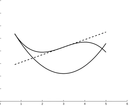
where (¯xi−1_{, ¯}_yi−1_{) is the solution of subproblem (}_P₁₎i−1 _and _Mk _{⊆ {}₁_{, . . . , m}} _{is the set} of (indices of) constraints from which OA cuts are generated from point (¯xk_,_y_¯k_{). We limit} the OA cuts added to (P2) because, when non-convex constraints are involved, not all the possible OA cuts generated are “safe”, i.e. do not cut off feasible solutions of (P) (see Figure 6.1).

(39)

2.2. THE ALGORITHM 21

(x0,y0)

Figure 2.1: Outer Approximation constraint cutting off part of the non-convex feasible region. When the OA cut is generated from a convex and tight constraint gm(x, y) it is valid. Indeed, let z∗ _{be the feasible solution of step 2.A and let} _g

j(z)≤0 be the convex constraint that is tight to z∗_{. The OA constraint would be:} _∇g

j(z∗)T(z−z∗) ≤ 0. Note that since

gj is convex, this property holdsgj(x) +∇gj(x)T(y−x)≤gj(y) for each x,y in the domain where gj is convex. Then, ∀z ∈ P, gj(z∗) +∇gj(z∗)T(z−z∗) ≤ gj(z). Since gj(z) ≤ 0 is tight to z∗_{, we have} _g

j(z∗) = 0 and ∇gj(z∗)T(z−z∗) ≤ gj(z). ∀z ∈ P, gj(z) ≤ 0, then

∇gj(z∗)T(z−z∗)≤0 is a valid cut for the original problem.

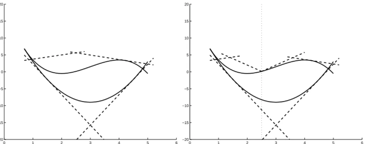
The problem with this involves basically two issues, one from a practical, the other from the theoretical viewpoint. The first issue is that discriminating convex and non-convex constraints is a hard task in practice. We will describe in Section 2.4 how we simplified this on the implementation side. The second issue is that Outer Approximation cuts play a fundamental role on convergence of the algorithm, i.e. if at one iteration no OA cut can be added, the algorithm may cycle. However, even if an OA cut is added, there is no guarantee that it would cut off the solution of the previous iteration, see, for example, Figure 2.2. In the figure, the non-linear feasible region and its current linear approximation. The solution of subproblem (P1) is ¯x and, in this case, only one Outer Approximation can be generated, the one corresponding to the tight and convex constraint. However, this OA cut does not cut off solution ˆx, but, in the example, the FP would not cycle, as the MILP at the next iteration would not pick out ˆx. This shows that there is a distinction between cutting off and cycling. However

We propose two solutions to this theoretical issue which will be described in the next two sections.

“No-good” cuts

One idea could be adding a constraint of the form:

kx−xk ≥ˆ ε , (2.13)

being valid for all feasible solutions of (P1), if valid for all integer feasible solutions, too. So it can be added to (P2) and it cuts off ˆx(of the previous iteration). The problem with constraint

(40)

ˆ x ¯ x x1 x2 γ

Figure 2.2: The convex constraint γ does not cut off ˆx, so nor does any OA linearization at ¯

x.

(2.13) is that it is non-convex. However, there are different ways to transform constraint (2.13) in a linear constraint. In general they are quite inefficient, but for some special cases, like the (important) case in which x∈ {0,1}n_{, constraint (2.13) can be transformed in:}

X j:ˆxi j=0 xj+ X j:ˆxi j=1 (1−xj)≥1 (2.14)

without requiring any additional variable or constraint. Defining the norm of constraint (2.13) as kk1 and because ˆxj can be only 0 or 1, in the first case kxj −xˆjk = xj, in the latter kxj −xˆjk = 1−xj, and we have, for ε= 1, equation (2.14). Exploiting this idea one can generalize the “no-good” cut valid for the binary case to the general integer case. The “no-good” cut for general integer variables reads as follows:

X j∈X:ˆxj=lj (xj−lj) + X j∈X:ˆxj=uj (uj−xj) + X j∈X:lj<xj<ujˆ (x+_j +x−_j)≥1, (2.15) where, for allj∈ X, we need the following additional constraints and variables:

xj = ˆx+x+j −x−j (2.16)

x+_j ≥ zj(uj−lj) (2.17)

x−_j ≥ (1−zj)(uj−lj) (2.18)

zj ∈ {0,1}. (2.19)

This leads to an inefficient way to handle the “no-good” cut, because 2nadditional continuous variables, nadditional binary variables and 3n+ 1 additional equations are needed.

(41)

2.2. THE ALGORITHM 23 This MILP formulation of the “no-good” cut for general integer can be seen as the interval-gradient cut of constraint (2.13) usingkk1 and ε= 1.

In the following we present some considerations about the relationship between the interval-gradient cut (see [98]) and the “no-good” cut proposed (2.15)-(2.19). Suppose we have a non-convex constraint g(x) ≤ 0 with x ∈ [x, x] and that [d, d] is the interval-gradient of g

over [x, x], i.e. ∇g(x) ∈ [d, d] for x ∈ [x, x]. The interval-gradient cut generated from this constraint with respect to a point ˆx is:

g(x) =g(ˆx) + min d∈[d,d]

dT(x−xˆ)≤0. (2.20)

(Here we are exploiting the following property: g(x) ≤ g(x) ≤ 0, then we know the cut is valid.) Equation (2.20) can be reformulated with the following MILP model:

g(ˆx) +X j∈X (dx+−dx−)≤0 (2.21) x−xˆ=x+−x− (2.22) x+_j ≤zj(xj−xj) j∈ X (2.23) x−_j ≤(1−zj)(xj−xj) j∈ X (2.24) x+≥0, x− ≥0 (2.25) z∈ {0,1}n (2.26)

with the cost of 2nadditional continuous variables, nadditional binary variables and 3n+ 1 additional constraints. Now, consider equation (2.13). It is non-convex and we try to generate an interval-gradient cut with respect to point ˆx. We first transform equation (2.13) in this way (using kk1 and ε= 1):

g(x)≤g(x) =−X

j∈X

|xj −xˆj| ≤ −1 . (2.27)

First consideration: g(ˆx) = 0. Now let analyze a particular index j ∈ X. Three cases are possible:

1. ˆxj =xj: this implies that−|xj−xˆj|= ˆxj−xj and d=d=−1. The term (dx+j −dx−j ) become −x+_j +x−_j =−xj+ ˆxj =xj −xj.

2. ˆxj =xj: this implies that−|xj−ˆxj|=xj−xˆj and d=d= 1. The term (dx+j −dx−j ) become x+_j −x−_j =xj−+ˆxj =xj−xj.

3. xj ≤ xˆj ≤ xj: this implies that d = −1 and d = 1. The term (dx+j −dx−j ) become

−(x+_j +x−_j).

We can then simplify equation (2.21) in this way: X j∈X:ˆxj=x_j (x_j−xj) + X j∈X:ˆxj=xj (xj−x) + X j∈X:x_j<xj<xjˆ (−x+_j −x−_j )≤ −1 (2.28)

(42)

changing the sign and completing the MILP model: X j∈X:ˆxj=xj (xj−xj) + X j∈X:ˆxj=xj (x−xj) + X j∈X:xj<ˆxj<xj (x+_j +x−_j )≥1 (2.29) x+_j ≤zj(xj−xj) j ∈ X (2.30) x−_j ≤(1−zj)(xj−xj) j ∈ X (2.31) x+≥0, x− ≥0 (2.32) z∈ {0,1}n (2.33) which is exactly the “no-good” cut for general integer.

In the following we present the details of how to linearize the “no-good” cut (2.13) in the general integer case. In particular we considered two cases:

1. Using k · k∞for problem (P1);

2. Using k · k1 for problem (P1).

We explicitly define the NLP problems for the two cases:

(N LP) (¯x,y¯) = argmin{ kx−xkˆ ∞ : g(x, y)≤0}= argmin{ε : −ε≤xi−xˆi ≤ε ∀i, ε≥0, g(x, y)≤0} (N LP) (¯x,y¯) = argmin{ kx−xkˆ 1 : g(x, y)≤0}= argmin{ε=X i vi : −vi ≤xi−xˆi≤vi ∀i, v≥0, g(x, y) ≤0}. In both the cases, if the objective function value of the optimal solution of NLP is equal to 0, we have an integer and feasible solution that is ˆx. If this is not the case, we have to solve the MILP problem, but we want to add something that avoid the possible cycling. If there are some convex constraints that are tight for (¯x,y¯), we can generate the OA constraints that is added to the MILP problem of the previous iteration and we will get a new (ˆxk,yˆk). If there is no convex constraint that is tight, we will solve one of these two problems (resp, for the

k · k∞ andk · k1 cases): (M ILPk) (ˆxk,yˆk) = argmin{ kx−xk¯ : gj(¯xk,y¯k) +∇gj(¯xk,y¯k)T x−x¯k y−y¯k ≤0 k= 1, . . . , i−1;j∈Mk, ⌈ε⌉ ≤xi−xˆki−1+M(1−zi) ∀i, ⌈ε⌉ ≤xˆk_i−1−xi+M(1−z′i) ∀i, X i zi+ X i z_i′ ≥1, z ∈ {0,1}p, z′∈ {0,1}p }

(Intuitively, if zi (or zi′) is equal to 1, the correspondent constraint is active and we impose that the componentiis changed wrt ˆxk−1₎

(M ILPk) (ˆxk,yˆk) = argmin{ kx−xk¯ : gj(¯xk,y¯k) +∇gj(¯xk,y¯k)T x−x¯k y−y¯k ≤0 k= 1, . . . , i−1;j∈Mk, vi≤xi−xˆki−1+M zi ∀i, vi≤xˆki−1−xi+M(1−zi) ∀i, X i vi≥ ⌈ε⌉, z∈ {0,1}p }

(43)

2.3. SOFTWARE STRUCTURE 25 (Intuitively, if vi is greater than 0, one of the 2 correspondent constraints is active and we impose that the component iis changed wrt ˆxk−1_{. The minimum total change is}_⌈ε⌉_).

where ε is the objective function value of the optimal solution of NLP, ˆxk−1 _{is the optimal}

solution of MILP at the previous iteration,M is the big M coefficient that has to be defined in a clever way.

Tabu list

An alternative way, which do not involve modifications of the model such as introducing additional variables and complicated constraints, is using a tabu list of the last solutions computed by (P2). From a practical viewpoint this is possible using a feature available within the MILP solver Ilog Cplex [71] called “callback”. The one we are interested in is the “incumbent callback”, a tool which allows the user to define a function which is called during the execution of the Branch-and-Bound whenever Cplex finds a new integer feasible solution. Within the callback function the integer feasible solution computed by the solver is available. The integer part of the solution is compared with the one of the solutions in the tabu list and, only if the solution has a tollerable diversity with respect to the forbidden solutions, it is accepted. Otherwise it is discarted and the Branch-and-Bound execution continues. In this way, even if the same solution can be obtained in two consequent iteration, the algorithm discarts it, then it does not cycle. It is a simple idea which works both with binary and with general integer variables. The diversity of two solutions, say, ˆx1 _{and ˆ}_x2_{, is computed in the}

following way:

X j∈X

|xˆ1_j −xˆ2_j|,

and two solutions are different if the above sum is not 0. Note that the continuous part of the solution does not influence the diversity measure.

2.2.3 The resulting algorithm

The general scheme of the algorithm proposed is described by Algorithm 2. The resolution of problem (P1) is represented by steps 10-27 and the resolution of problem (P2) is represented by steps 28-40. At step 23, a restriction of problem (P) is solved. This restriction is “generally” a non-convex NLP we solve to local optimality, if we have no assumption on the structure of the problem. The objective function problem of step 34 is kx−x¯i_k

1. Finally note that, if

use tabu list is 0, TL is∅and no integer solution will be rejected (the “no-good” cuts do the job).

In the next section we present details on the implementation of the algorithm.

2.3 Software structure

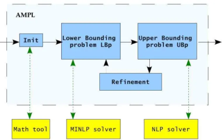
The algorithm was implemented within the AMPL environment [55]. We choose to use this framework to be flexible with respect to the solver we want to use in the different phases of the proposed algorithm. In practice, the user can select the preferred solver to solve NLPs or MILPs, exploiting advantages of the chosen solver.

The input is composed of two files: (i) the mod file where the model of the instance is implemented, called “fpminlp.mod”; (ii) the file “parameter.txt”, in which one can