Methods of the efficient state space search for the nurse rostering problem using branch-and-price approach

(1)

CZECH TECHNICAL UNIVERSITY IN PRAGUE

Faculty of Electrical Engineering

MASTER’S THESIS

Anton´ın Nov´

ak

Methods of the efficient state space search for the Nurse

Rostering Problem using branch-and-price approach

Department of Computer Science Thesis supervisor:Ing. Roman V´aclav´ık

(2)

(3)

(4)

(5)

(6)

(7)

Acknowledgements

I would like to thank my family for support during writing this thesis and throughout my studies. Without them this work would not be possible. Moreover, thanks belongs to my girlfriend who patiently supported me over the years and provided me a calm environment for my work. Furthermore, I would like to thank my thesis supervisor and Pˇremysl ˇS˚ucha for great insights and discussions. Finally, my thanks goes to my friend Tom´aˇs B´aˇca for his excellent comments and helpful corrections.

(8)

(9)

Abstract

This thesis introduces an exact algorithm for Nurse Rostering Problem based on general decomposition method called Branch and Price. Pro-posed method handles expressive set of soft constraints and is suitable for real-world personnel rostering problems, which is shown by evaluation on publicly available benchmark instances collected from real-world environments. Furthermore, we have shown, how solutions of related hard optimization problems can be used for future ones. Moreover, we studied problem in details and proposed number of improvements, that made proving optimality of solutions tractable for medium-sized instances.

Keywords: nurse rostering problem, branch and price, combinato-rial optimization

Abstrakt

Tato práce popisuje exaktn´ı algoritmus pro problem rozvrhován´ı zdravotn´ıch sester zaloˇzený na obecné dekompoziˇcn´ı metodˇe Branch and Price. Popsaný pˇr´ıstup zvládá ˇsirokou ˇskálu mˇekkých omezen´ı a je vhodný pro nasazen´ı v reálných prostˇred´ıch, coˇz je doloˇzeno testován´ım na veˇrejných instanc´ı problému z reálných prostˇred´ıch. Mimo jiné jsme ukázali, jak ˇreˇsen´ı pˇr´ıbuzných tˇeˇzkých optimalizaˇcn´ıch úloh mohou pomoci pro ˇreˇsen´ı tˇechto problém˚u v budoucnu. Studovány byly také vlastnosti problému, na základˇe kterých jsme navrhli vylepˇsen´ı, které vedly k dosaˇzitelnosti prokazován´ı optimality na instanc´ıch stˇredn´ı velikosti.

Kl´ıˇcová slova: problém zdravotn´ıch sester, branch and price, kom-binatorická optimalizace

(10)

(11)

CONTENTS

List of Figures

1.1 Illustrative comparison of computation runtime of polynomial algorithms

(ma-trix multiplication, sorting) and an exponential one (Nurse Rostering). . . 2

1.2 Example solution of Valouxis instance (Valouxis and Housos, 2000). . . 4

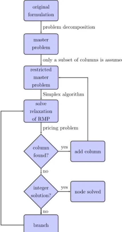
2.1 Block diagram of the branch and price algorithm. . . 12

2.2 New variables and their meaning. . . 15

2.3 Primal master model. . . 17

2.4 Dual master model. . . 19

2.5 Column generation procedure. It generates a new column that could improve primal objective based on the current dual solution. . . 20

2.6 Optimization in dual space over 3 variables. Displayed polytope is a feasible region of dual LP. Inserting a cutting plane (a new schedule) (see Figure 2.6b) makes current dual solution infeasible, thus it lowers the dual objective value and consequently reduces the primal objective. . . 22

3.1 An example of a pattern matching in a schedule. . . 25

3.2 Graph structure for the pricing problem. Vertical layers correspond to days and vertices to shift types. We are interested in finding the cheapests−tpath which satisfies given constraints. . . 26

3.3 An illustrative example of the search tree with some dominated partial solu-tions. Consider a constraint where we want to have at least two E shifts in schedule. Partial scheduleEDDis dominated byEEN,EDNis dominated by ENE. 29 3.4 An illustrative example of resources. Partial solution NE-N is associated with resource vector [−200,0,1]. The first element is associated with the partially evaluated reduced cost, the other are resources associated with constraints a) and b). Dominance procedure compares vectors of corresponding partial solutions element by element. . . 29

3.5 Example of an automaton rejecting On-Off-On pattern. Initial state is S0, accepting states areS0...2. . . 35

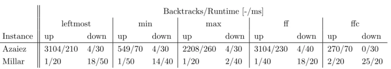
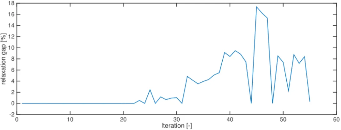
3.6 LP relaxation is tight. Example gap between IP optimum and LP solution for Azaiez instance. . . 37

4.1 An example of coverage penalties. . . 41

4.2 An example of a single-pass initial heuristics. A new column (t+1) is created based on the dual multipliers calculated by coveragesR(_mjkt) satisfied up to (t). 43 4.3 Lower bound computed by Lagrangian relaxation at each iteration of column generation inMillar instance. . . 45

(16)

LIST OF FIGURES

4.4 Example of 0–1 branching with the most fractional value variable selection. It creates exactly two branches — in the first one it forbids the assignment and in the second one it fixes the shift for a specific day and employee (and consequently forbids other shifts for the same day). Fixed assignments are in

bold. . . 47

4.5 Example of 1/../S branching. For each possible shift assignment for a given day it creates a new branch with fixed value. Fixed assignments are in bold. . 48

5.1 Example of loss function for a single datapoint,= 0.5 . . . 55

5.2 Discounting function for previous datapoints . . . 55

5.3 Upper bound prediction for subproblems in Millar instance. . . 58

5.4 Upper bound prediction for subproblems in Azaiez instance. . . 59

6.1 Unstabilized column generation inMillar instance. Distance from current dual solution to optimal dual solution is not monotonically decreasing. It results in so-calledbang-bang behavior. . . 61

6.2 An illustrative example of symmetry breaking. It fixes single assignment for 3 different employees. . . 67

7.1 Optimal solution for Motol-1 instance. Large consecutive blocks of free days are caused by personal requests (i.e. vacation). . . 73

(17)

1 INTRODUCTION

1 Introduction

Assigning employees to shifts in workplaces is a problem that is being solved every day on the entire planet. Usually, every place that is running operations involving larger number of people creates a working schedule for them, typically a few weeks onwards. Such working schedule specifies what the duty of an employee is for any given day. Knowing this in advance is important both for employees to arrange their personal activities and for the manager and the company to plan the production.

Imagine for example a department in a large-sized hospital. The task of the head nurse is to ensure that the department is able to provide high-quality health care every day of the year. It means that employees of desired qualification come to work every day so that there is always e.g. someone who can operate an X-Ray machine and that there are at least 5 nurses in the morning and at least 3 nurses in the afternoon. Furthermore, the head nurse has to ensure that employees are not tired and can perform to their best.

However, the hospital has limited staff only. These people also have custom working con-tracts specifying different number of hours per month they are allowed to work. Moreover, some of the employees have planned vacation, some nurses cannot work at night or they would miss the last bus home, and some nurses have a small child, so they have to take them to school every morning.

The head nurse cannot plan shifts for employees in an arbitrary way. Hospital staff does not want to work too long without a rest period and, moreover, there are also working regulations given by the working union and the labor code which have to be obeyed.

Although it may seem that the motivation includes the nurses in hospitals only, the con-verse is true. The same problem, scheduling of human resources, is appearing frequently in production, services and other areas of industries where a large number of employees occur. For example, similar problem is being solved in large modern cinemas. A cinema typically employs tens of employees which need to be scheduled over a time period. There are different shift types (morning, day and night shift) and people are trained for different positions (selling tickets, selling food and drinks, welcoming customers, etc.). Moreover, different staffing de-mands are imposed for different times and days. This and other similar problems can be easily reduced to our problem. Therefore, they can be solved by the same algorithms. Thus, Nurse Rostering Problem is not an artificial example just made up by researches, but it addresses the very important and practical problem of general personnel rostering.

If the (e.g. monthly) schedule for all employees has to be created by hand, the person in charge of it will not only spend a lot of time while doing that but the solution is likely to be far from optimal. The solution by hand can easily take hours to get while a computer might

(18)

1 INTRODUCTION

be able to find a better one in the order of minutes. Thus, it makes sense to pass this task over to the computer.

However, this task is hard even for current computers. Properties of Nurse Rostering Problem make it fundamentally different from problems like sorting a set of numbers (which is still time demanding for a human being, but computers are able to do it quickly) or finding a book in a digital library which can be solved easily. Informally said, Nurse Rostering Problem reaches a level of complexity which our computers are not able to solve fast in general. This complexity level is calledN P-hard. Simply said, if a problem isN P-hard, it means that, in general, we do not know how to solve it in polynomial time1 with respect to input length. Commonly, solution of these hard problems takes a long (exponential) time. Nowadays, only algorithms with exponential time complexity for solving N P-hard problems are known.

Instance size Time Nurse Rostering

Matrix multiplication Sorting

Figure 1.1:Illustrative comparison of computation runtime of polynomial algorithms (matrix multiplication, sorting) and an exponential one (Nurse Rostering).

When facing such a complex problem, theexponential blow upmust be pushed to the right side (extending the plateau where instances can be solved reasonably fast) as far as possible (see Figure 1.1), so that problems of desired sizes can be solved in reasonable time. It can be done by studying the problem carefully in detail and looking for its properties and structure that can be exploited.

Even though we call this problem Nurse Rostering due to historical reasons (nurses have one of the most complicated labor codes, thus the study of this domain is challenging), one has to keep in mind that many personnel rostering problems are reducible to our problem.

The last question to answer is whether the problem introduced above needs to be solved optimally or if a heuristic (suboptimal) solution is sufficient. Many will argue thatanysolution for a rostering problem is essentially sufficient when one is able to obtain it quickly. However, we claim that if we were able to get the optimal solution in a comparable time, there is no

(19)

1 INTRODUCTION

reason to use the suboptimal solution.

In this thesis, we study the general variant of Nurse Rostering Problem (Burke et al., 2004) and we show its properties that allow us to solve real-world instances optimally in the order of minutes.

1.1 Problem statement

We are given a planning horizon of lengthn, a set of employeesE, a set of skill competencies J and a set of a shift typesK. For each employee i∈ E we have a set of patterns P_i which defines both desirable and undesirable shift sequences. Each pattern is defined by a regular language and is associated with a start day, a lower and upper limit for its appearance in i’s individual schedule and a cost and penalty function for violating it (see Table 1.1). Each employee can also specify their preference for assignment to each shift type on each day. Moreover, employee i can be associated with a permitted workload. A workload specifies a minimum and maximum number of time units (thus each shift typek∈ Kis associated with some time units, i.e.shift duration) allowed and the penalty for violation. Since the workload can be also specified over subintervals of the planning horizon, an employee can be associated with multiple workload constraints simultaneously.

The set of pattern based constraintsPi and the workload constraints combined together is

called aworking contract. In general, there are two types of constraints — hard constraints and soft constraints. Hard constraints must be satisfied at all cost. These can be some forbidden shift patterns given by a labor code or minimal workload specified by a working contract. Different hard constraints are given by the limitations of real world (i.e. every employee can serve at most one shift at the same time) or by the problem description (i.e. every employee has exactly one skill).

Soft constraints are the ones that can be violated for some penalty. In Nurse Rostering Problem, these are pattern based constraints in most cases. Table 1.1 provides an example of pattern based soft constraints and calculation of the penalty. The other common soft constraint is the maximal workload. In contrast to the minimal workload constraint, working overtime is common. However, the employer must pay to those employees more money, which is undesirable from the company’s budget point of view.

Moreover, we are given a requirement for the preferred coverageRmjkassociated with the

day m, served by employees with the skill competency j on the shift k for each day of the planning horizon. It is linked with the penaltycu

mjkfor understaffing andcomjkfor overstaffing

it. We can also be given a minimum and maximum staffingM Imjk(M Amjk respectively) and

(20)

1 INTRODUCTION

Description Pattern Penalty Schedule Cost

Max 3 consecutive N No 4 N NNNN 5, linear function N N N N N 10 No N after E No EN EN 20, linear function N E E E N 20

Max 2 days off

No - - - 2, quadratic function

N - - -

-8 Table 1.1:Examples of pattern soft constraints for the individual employee and their calculation. Nstands for night shift,Efor early shift and-denotes a day off.

are specified, the combined penalty function is used. Notice, that these are soft constraints also. For detail treatment of coverage penalties see Figure 4.1.

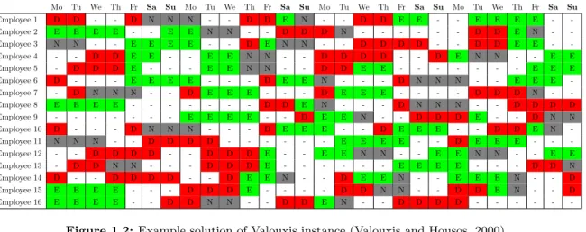
The objective is to minimize the sum of constraint violations (patterns) for each employee plus sum of violations of their shift requests plus sum of violations of coverage constraints. Nurse Rostering Problem is commonly modeled by a nurse-day view (Cheang et al., 2003). That is matrixX where each row corresponds to a nurse and each column to a specific day. Thus, nurseiis assigned to shiftxij on dayj. Such matrix of the solved problem can be seen

in Figure 1.2. Mo Tu We Th Fr Sa Su Mo Tu We Th Fr Sa Su Mo Tu We Th Fr Sa Su Mo Tu We Th Fr Sa Su Employee 1 D D - - D N N N - - D D E N - - D D E E - - E E E E - -Employee 2 E E E E - - E E N N - - D D D N - - - D D E N - -Employee 3 N N - - E E E E - - D E N N - - D D D D - - D D E E - -Employee 4 - - D D E E - - E E N N - - D D D D - - D E N N - - E E Employee 5 - D D D E - - - E E N N - - D D E E - - - E E E Employee 6 D - - - E E E E - - - D E E N - - - D N N N - - E E E -Employee 7 - D N N N - - D E E E - - - D E E E - - - - D D D N - -Employee 8 E E E E - - - D D E N - - - D N N N - - D D D D Employee 9 - - - E E E E - - D E E N - - D D D E - - D N N Employee 10 D - - - D N N N - - - D E E E - - D E E E - - D D E N -Employee 11 N N N - - D D D D - - - E E E E - - D E E E - - -Employee 12 - - D D D D - - D D D E - - E E N N - - E E N N - - E E Employee 13 - D D N N - - - D D D E - - - E E E E - - - D D N Employee 14 D - - D D D D - - D E E N - - D E E N - - E E E N - - D Employee 15 E E E E - - - D D D E - - - - D D N N - - D D E N - - D Employee 16 E E E E - - D D N N - - D D E N - - D D D D - - -

-Figure 1.2: Example solution of Valouxis instance (Valouxis and Housos, 2000).

We call this matrix the roster. When we speak about the individual schedule of an em-ployee, we are referring to the corresponding row in the roster.

(21)

1 INTRODUCTION

1.1.1 Difficulties in practice

Many researchers did not address the problem in a way closely related to the real-world environments (Burke et al., 2004). Since the problem is too complex, algorithms tend to adopt simplifying assumptions making the problem easier to solve. A large number of approaches assume a custom (hand-picked) set of constraints or treat them as hard ones. These assump-tions often make problems not well-suited for different environments — it is common that hospital’s departments have different requirements and staff’s habits, therefore, some practice which is forbidden at some places may be allowed in other ones.

However, due to a large number of restrictions for individual schedules it can easily happen that no solution can meet all the demands, i.e. the problem becomesoverconstrained. In order to find at least some solution, we have to allow to violate constraints for somepenalty. Thus, it is reasonable instead of (hard) constraints to assumesoft constraints (the ones that can be violated even though it is not preferred).

Treating constraints as soft ones gives employer sufficient freedom for the design of the constraint set and other requirements given by the problem description. On the other hand, the issue with defining costs for violations arises. The individual nurse’s preferences from their point of view can be more important than for a head nurse who is responsible for a proper staffing. The other obvious issue is that violation of some constraints is hardly comparable (e.g. how to compare penalty for understaffing on the morning shift to the violation of working regulations?).

The usage in practice of flexible approaches allowing soft constraints can be difficult due to questions raised above. However, we believe that the high quality of rosters produced by those algorithms greatly pays off for itself (especially when the solutions are optimal ones like with our approach) and makes flexible approaches useful even though some parameters (penalties) must be supplied.

1.1.2 Computational complexity

The task of solving the problem described above even for just one employee can be identi-fied asN P-hard. It can be shown that reduction from 3-SAT to NRP takes polynomial time (see Chapter 3.2). This means that we cannot find a polynomial algorithm for solving NRP unlessP =N P.

Fortunately, we can exploit the inner structure of the problem in order to speed up the algorithm. Complex constraints for the individual schedules are specified for single employee only, thus these constraints can be resolved independently. These individual employees’

(22)

sched-1 INTRODUCTION

ules are then tied up with coverage constraints which are much simpler to solve. This structure results in a block-diagonal constraint matrix in IP (integer programming) formulation, which can be solved much faster than some dense, highly coupled problems.

1.2 Related work

Nurse Rostering Problem has a long history counting more than 40 years. Methods de-veloped so far can be split into two categories — heuristic and exact. Naturally, the heuristic ones were adopted earlier because they are able to handle larger instances in tractable times. Heuristic approaches for Nurse Rostering Problem cover metaheuristics, methods based on mathematical programming and many others.

The other category of approaches, the exact ones, is considerably smaller. Most of the authors did some simplifying assumptions on the constraints or the staff requirement in order to solve the problem. For example, soft constraints are not always assumed. The issue is that most of these modifications simplify the problem too much to be applied successfully in practice, i.e. in real-world environments.

Essentially, all approaches published until recent time are the heuristic ones or assumed a limited constraint set. Those which did not, will be also described in the paragraphs below.

The (Warner and Prawda, 1972) and (Warner, 1976) are early publications on a heuristic method based on the mathematical programming for Nurse Rostering Problem. It allowed to specify weights for constraints (undesired patterns) in the schedule. Some assignments were made by hand (shifts at weekends etc.) before the optimization. The algorithm had 2 stages — it searched for a feasible solution first and then it tried to find an improvement. This algorithm was employed in several hospitals across the U.S.

In Nurse Rostering Problem, there are obviously often many conflicting goals — e.g. to minimize the difference between desired and scheduled staff coverages, to maximize per-sonal preferences, to minimize labor costs, etc. Thus, some multi-criteria approaches emerged. (Jaszkiewicz, 1997) used a semi-interactive approach. The method used two stages — the first stage ran simulated annealing (pareto-simulated annealing) and the second one was an in-teractive stage, where the human operator selected good solutions by hand. Therefore, the scheduling process was not fully automated.

(Jaumard et al., 1998) showed an approach based on column generation and branch and bound. The objective was to minimize salary cost and employee dissatisfaction subject to cov-erage demands. The subproblem (finding schedule for given nurse) was aresource constrained shortest pathproblem with a non-decreasing resource function (Irnich and Desaulniers, 2005).

(23)

1 INTRODUCTION

Authors assumed a fixed constraint set including workload, shift rotations, etc. Their paper reported that the proposed method was olny able to find feasible solutions, not necessary op-timal ones. However, this work was an important improvement towards the exact approaches. For solving real-world problems, a considerable number of metaheuristic approaches was successfully applied. (Burke et al., 1999) introduced a hybridized tabu search and human-inspired techniques for an improvement of solutions. (Burke et al., 2001) described a set of genetic and memetic algorithms where coverage constraints are satisfied throughout the whole search. The proposed method handled complex constraints and requirements for staffing. The introduced recombination operator was based on hand-crafted characteristics of the solutions. However, the approach suffered from long running times. (Aickelin and Dowsland, 2000, 2004) proposed an indirect genetic algorithm where the constraints are expressed as a set of feasible patterns. (Ikegami and Niwa, 2003) used a mathematical programming formulation solved by tabu search. The approach was used in order to solve problems in Japan’s hospitals, thus it implemented specific work regulation requirements. The problem is decomposed into subproblems, where all but one nurse are fixed. However, the proposed approach is also heuris-tic. (Burke et al., 2010) introduced hybridized heuristic ordering with variable neighborhood search (Mladenovi´c and Hansen, 1997). The method is able to support rostering decisions in large modern hospital environments. The proposed approach offered good balance between quality of solutions and computation time, allowing expressive problem formulations.

(Petrovic et al., 2003) used case-based reasoning, where the problems are solved based on past experience. The approach imitated the human style of reasoning about rostering (Burke et al., 2004). Only a limited set of rules for the roster was permitted, although it was applied in practice.

The (Menana and Demassey, 2009) showed an interesting improvement for the Constraint Programming model, where undesired patterns in the individual schedules are modeled as fragments of a regular language. Authors designed a custom global constraint encapsulating

the regular and gcc (global cardinality constraint) global constraints in order to speed

up domain propagation. Moreover, they used Lagrangian relaxation for filtering domains. It greatly improved runtime, however, the model handled hard constraints only.

(Maenhout and Vanhoucke, 2010) described an exact method based on the branch and price algorithm. The proposed model allowed preferred coverage requirements (2-piecewise linear penalty) over single skill competency and assumed hard constraints only, which allowed reasonable solving times. Moreover, authors explored various branching strategies. They used a custom artificial dataset for testing performance.

A branch and cut method was used for solving one of the modifications of Nurse Rostering Problem in International Nurse Rostering Competition 2010 in (Santos et al., 2014). The

(24)

1 INTRODUCTION

authors implemented a custom cut generation procedure for clique cuts. They proposed an approach where instead of finding the most violated cut they add all violated cuts at once. (Burke and Curtois, 2014) presented a method based on branch and price algorithm. It was able to solve real-world benchmark instances (Curtois, 2014). Their algorithm handled various soft constraints and expressive problem formulations. However, even though authors used the branch and price algorithm, which in general is an exact method, Burke’s method is not exact in our opinion. We present arguments supporting this claim in Chapter 1.3.

1.3 Summary

Nurse Rostering Problem is greatly complicated. As (Tien and Kamiyama, 1982) men-tioned:”nurse rostering is more complex than the traveling salesman problem . . . ”. The devel-opment of an exact algorithm, which is able to solve real-world instances up to the optimality is a rather challenging task. Thus most of the approaches to Nurse Rostering Problem are heuristic — ”most of these approaches are not exact” . . . ”problem is too complex” (Burke et al., 2004).

The objective is to minimize the sum of the penalties for violation of individual preferences, work regulations, coverage constraints and shift patterns in individual schedules in most cases. Thus, it is desired to treat constraints as soft ones. In our opinion, it is a more faithful description of reality. However, it makes the problem more difficult. Although it may not be obvious, problems with soft constraints are harder to solve than the ones with hard constraints only. When one is solving the problem optimally, hard constraints can be used for effective pruning of the search space, which cannot be done with soft constraints easily.

When one is looking for the best solution of the roster, the aim is to design an algorithm forproving its optimality in a short runtime. In order to find the optimal solution, the solution with the lowest objective value has to be found and moreover, the proof that there is no other with lower objective value is needed. This is hard in this domain and it makes the problem challenging. To get some sense about particular numbers, the typical instance has about 20 employees, a 4 week planning horizon with 4 shift types and about 15 soft constraints per employee. This forms a search space of a size approximately 21120 ≈10337 where each state (solution) is feasible. In order to solve such instances up to the optimality, one has to reason intelligently about which parts of the search space are actually useful and prune other parts aggressively.

For finding the exact solution of Nurse Rostering Problem, the integer programming is usually a method of choice. In our opinion, the branch and price approach is more flexible than the branch and cut. It permits more complicated constraints, which could be hard to put

(25)

1 INTRODUCTION

into general integer programming model. Therefore, the branch and price approach is more suitable for solving real-world instances.

To the best of our knowledge, the only work on Nurse Rostering Problem solved by the branch and price approach which is evaluated on real-world benchmark instances (Curtois, 2014) was published by (Burke and Curtois, 2014). The authors briefly described a basic variant of the branch and price approach but the description of arguably the most important part of the algorithm, the pricing problem, lacks details. Moreover, its description contains mistakes — in the dominance procedure, lower bound on the reduced cost is not mentioned, which is a crucial detail that was omitted. Moreover, we were not able to reproduce the results achieved by their pricing procedure, thus we assume that some important details were omitted (one clear example is the calculation of the lower bound which is missing completely, see Chapter 3.3.1 for more details). Moreover, authors avoided the statement, whether their approach is exact or heuristic. The article creates the impression that it presents an exact method, since the branch and price is commonly used as the exact one. However, the results show that their algorithm sometimes seemingly randomly stops without reaching any maximal run time limit. The same behavior can be observed in the results for different benchmark data presented in (Curtois T., 2014). In this work, authors more or less admitted that their approach is not able to always find the optimal solution, although time or memory limits are not exceeded. Therefore, it seems that they employed some speedup techniques (e.g. rounding up some decision variables, which prevents from backtracking) while sacrificing the completeness of the algorithm and those techniques were not described in the paper.

Even though their algorithm was able to find the optimal solution for the majority of real-world test instances, it is a simplified task without proving their optimality. To see the dif-ference betweenfinding the optimal solution andproving its optimality, consider e.g.Golomb ruler problem (Smith et al., 1999). For example, the optimal ruler of order of 26 was found in 2007 using a large cluster of computers, but its optimality was proven nearly two years after its discovery2.

However, (Burke and Curtois, 2014) presents the best known results and we will compare ourselves to those even though it is not clear whether their approach is exact.

1.4 Contribution

We have designed an exact algorithm for solving Nurse Rostering Problem which allows pattern based soft constraints, coverage requirements with 4-piecewise linear penalties, soft workload constraints and employees’ preferences. The method is based on the branch and price

(26)

1 INTRODUCTION

approach, whose parts were further improved. We validated results on real-world benchmark data (Curtois, 2014).

Beside achieving better results than in (Burke and Curtois, 2014) we further explored the possibilities of applying the knowledge gained during the run of the algorithm in order to decrease the computation time. Moreover, our contribution consists of solving a new real-world instance for the surgery department ofMotol hospital in Prague, Czech Republic (see Chapter 7.2). We were able to find the optimal schedule for their department in a few minutes and we improved the overall quality of their roster’s objective by a factor of over 220. More specifically, our contribution consists mainly of:

• a new LP formulation of a master model allowing minimal and maximal staffing levels across subsets of skills (see Chapters 4 and 2.4.1) and featuring a novel symmetry breaking technique (see Chapter 6.4)

• a MIP based pricing model with a number of improvements containing branching prior-ities and dynamical control of precision level based on the convergence of master model (see Chapter 3.3.2)

• the proof that the decision version of the pricing problem with soft constraints is N P -complete and is not polynomially approximable within(see Chapter 3.2)

• new initiation heuristics (see Chapter 4.2) and new primal heuristics for obtaining upper bounds (see Chapter 4.6)

• a number of improvements to column generation applied to Nurse Rostering Problem, mainly subproblem skipping and earlier branching (see Chapters 6.3.4 and 6.2.3) • a novel machine learning algorithm for upper bound prediction in the pricing problem

(see Chapter 5.2)

1.5 Outline

The rest of the thesis is organized as follows. Chapter 2 presents an overview of the general branch and price algorithm and column generation. Then, we show how to apply it to Nurse Rostering Problem and we derive some important equations. In Chapter 3, thePricing Problem is defined and its computational complexity is proven. We show solution methods, both exact and heuristic ones. It concludes with noteworthy aspects of the problem. Chapter 4 defines the Master Problem. Initiation heuristics are discussed as well as various branching schemes. In Chapter 5 we deal with opportunities for application of machine learning methods to problems in combinatorial optimization. We show how the knowledge gained during the

(27)

1 INTRODUCTION

column generation may be applied for future problems. Chapter 6 presents topics concerning effective usage of the branch and price algorithm we have discovered. The thesis concludes with experimental evaluation in Chapter 7 and states ideas for future research in Chapter 8.

(28)

2 BRANCH AND PRICE METHOD

2 Branch and price method

The purpose of this chapter is to introduce the reader to the column generation and branch and price algorithm as a whole. We will show an interpretation of column generation using duality and the application of branch and price approach to Nurse Rostering Problem. The more detailed treatment of branch and price approach to the general integer programming problem is nicely described in (Barnhart et al., 1998).

2.1 General overview

This chapter describes the branch and price method (Barnhart et al., 1998). It consists of several parts, which will be later described individually in separated chapters. The diagram of the algorithm can be seen in Figure 2.1. Before the problem can be solved by branch and price, one has to decompose the original problem (original formulation) to amaster problem. Informally, master problem is a linear program that consists of variables related to all feasible states of a state space given implicitly by the original formulation. This usually means, that the master problem is huge (typically it has exponentially many variables in terms of number of original formulation’s variables).

original formulation master problem restricted master problem solve relaxation of RMP column

found? add column

integer

solution? node solved

branch

problem decomposition

only a subset of columns is assumed

Simplex algorithm pricing problem no yes yes no

(29)

However, since only a few of these new variables are non-zero in an optimal solution, it is natural to not consider them all at once. When only a subset of them is considered, we get a restricted master problem. Throughout the optimization process, we repeatedly insert new variables (columns) to the restricted master problem until the point, where one is able to prove, that it represents an optimal solution of the master problem itself (i.e. no additional columns are required).

In case that this solution is integer, it also represents a solution of the original formulation. If it is not, one has to split the search space into disjoint parts and repeat the procedure for each part. By examination of all nodes which yielded with an integer solution we can ensure that we find the optimal one.

2.2 Original formulation

The problem described in Chapter 1.1 can be modeled as an integer programming problem. The most straightforward formulation is to use binary decision variables for assigning people to a shift on specific day. We will refer them asx in the rest of the text. A model based on these decision variables is not very good for two reasons — first of all, it contains a lot of symmetries (see Chapter 6.4 for more details) and secondly, it has weak linear relaxation.

We will show both the original formulation of the problem and its decomposition on a simple example. Consider following problem — we have 2 identical employees to be scheduled over 4 days. There are only day shift D and day off (denoted as −). Each employee has constraints that they can work only 1 or 2 days and can has 2 or 3 days off. Each violation of these constraints is penalized with 1 (unit penalty). For each day we require that there is at least one employee on D shift with penalty 5 for understaffing.

Using the originalx variables, we could model this problem in following way min x,p,n X e∈{1..2} po_e,₀+po_e,₁+pu_e,₀+pu_e,₁+ X m∈{1..4} 5nu_m,₁ (2.1) subject to ∀e∈ {1..2}: X m∈{1..4} xem0≥ 2−pue,0 (2.2) ∀e∈ {1..2}: X m∈{1..4} xem0≤ 3 +poe,0 (2.3) ∀e∈ {1..2}: X m∈{1..4} xem1≥ 1−pue,1 (2.4) ∀e∈ {1..2}: X m∈{1..4} xem1≤ 2 +poe,1 (2.5)

(30)

2 BRANCH AND PRICE METHOD ∀m∈ {1..4}: X e∈{1..2} xem1 ≥ 1−num,1 (2.6) ∀e∈ {1..2},∀m∈ {1..4}:xem0+xem1= 1 (2.7) x∈ {0,1}2×4×2 _(2.8) p,n ≥ 0 (2.9)

where variablexemk is equal to 1 if and only if the employeeeis assigned to shiftk(denoting

k= 0 as day off) on daym. Variable pu

e,k (poe,k) is associated with the penalty for violations

of lower limit (upper limit respectively) for the number shiftk for employee e. Finally,nu_m,₁ is slack variable for understaffing on daym.

Constraints (2.2) through (2.5) compute quality of individual schedules via penalties p and constraint (2.6) is defining the penalty for understaffing on each day.

Instead of above formulation, we will use more efficient one by exploiting special structure in the problem making it solvable efficiently.

2.3 Reformulation for Nurse Rostering Problem

The same problem as in previous chapter can be formulated in following way

min y,n 2 X i=1 16 X j=1 cijyij+ 4 X m=1 2 X k=1 5nu_mk (2.10) subject to ∀i∈ {1..2}: 16 X j=1 yij = 1 (2.11) n ≥ 0 (2.12)

(31)

2 BRANCH AND PRICE METHOD cij: 2 0 0 0 0 0 0 2 0 0 0 2 0 2 2 4 - - - D D D D D D D D - - - - D D D D - - - - D D D D - - D D - - D D - - D D - - D D - D - D - D - D - D - D - D - D y1,1 y1,2 y1,3 y1,4 y1,5 y1,6 y1,7 y1,8 y1,9 y1,10 y1,11 y1,12 y1,13 y1,14 y1,15 y1,16 cij: 2 0 0 0 0 0 0 2 0 0 0 2 0 2 2 4 - - - D D D D D D D D - - - - D D D D - - - - D D D D - - D D - - D D - - D D - - D D - D - D - D - D - D - D - D - D y2,1 y2,2 y2,3 y2,4 y2,5 y2,6 y2,7 y2,8 y2,9 y2,10 y2,11 y2,12 y2,13 y2,14 y2,15 y2,16

Figure 2.2:New variables and their meaning.

Each of these variables is related to some individual schedule for its employee and is associated with the cost of that schedule. Selecting a variable contributes to the coverage constraints included in the model.

0y1,1+ 0y1,2+· · ·+ 1y1,16+ 0y2,1+ 0y2,2+· · ·+ 1y2,16≥1−nu1,1 (2.13)

0y1,1+ 0y1,2+· · ·+ 1y1,16+ 0y2,1+ 0y2,2+· · ·+ 1y2,16≥1−nu2,1 (2.14)

0y1,1+ 0y1,2+· · ·+ 1y1,16+ 0y2,1+ 0y2,2+· · ·+ 1y2,16≥1−nu3,1 (2.15)

0y1,1+ 1y1,2+· · ·+ 1y1,16+ 0y2,1+ 1y2,2+· · ·+ 1y2,16≥1−nu4,1 (2.16)

Denoting left-hand-side of constraints (2.13) to (2.16) as matrix A, the entry aij takes

value 1 if the j-th schedule assigns D shift on i-th day and 0 otherwise. One of the optimal solutions of the problem (2.10) is y1,4 = 1, y2,13 = 1 with the objective value 0 since it is a

lower bound on the objective.

Having all schedulesyij enumerated explicitly wouldn’t help us to solve the problem faster

since there is an exponential number of them. Instead of it, we will only consider a subset of them and generate new ones on demand. So, ideally, we would generate only exactly 2 of them (y1,4 and y2,13) out of 2×16 = 32. Therefore, the linear program would be tiny and it

will be solved efficiently.

The example shown above can be generalized as follows (Desrosiers and L¨ubbecke, 2005). Consider following general form of linear programming problem

min

x c

T_x _(2.17)

subject to

(32)

x∈ X={x∈_Zn|Fx≤w}

For the decomposition we use the fact that constraints specified by matrixAareeasyto solve on their own but the constraints in matrixFare the difficult ones. For our problem it holds thatA ≈coverage constraints and F ≈ work regulations constraints.

Furthermore, the latter one is a block-diagonal matrix since the work regulations for individual schedules are not coupled to each other. We exploit this structure by following informal description — themaster model will take care of constraints in the matrix A and the so-calledpricing model will repeatedly solve the task of finding individual schedules for employees such thatFx≤w holds. Correspondingmaster problem is then

min λ X l∈L clλl (2.18) subject to X l∈L alλl≤b (2.19) ∀l∈ L:λl≥0 (2.20)

Decomposed model into this structure can be then solved efficiently bycolumn generation

(Desrosiers and L¨ubbecke, 2005). This method solves the problem by generating columns into matrixA and coefficients into vector c iteratively. At each iteration it solves problem based on the dual formulation of (2.18) in form of minl∈L{cl−πTal} = minx∈X{c(x)−πTa(x)}

subject to that costclof a columnal is given by the structure of the problem described by the difficult constraintsFx≤w. Theπdenotes dual prices for the constraints (2.19). Therefore, difficult constraints are not present explicitly in the decomposed model.

In our problem, each column corresponds to a complete working schedule for one em-ployee. Since all the possible columns are not present explicitly inA, new ones are added in iterative way. Furthermore, only the schedules, which are useful for the master model accord-ing to the coverage constraints can be considered. By addaccord-ing these useful schedules (columns) iteratively, we converge into the optimal solution without enumerating all of them. This is one of the sources of efficiency of column generation method. More detailed treatment of column generation is presented in Chapter 2.6.

So far, we have talked only about column generation itself. One has to keep in mind, that column generation is a continuous optimization method, thus it does not ensure integer property of the solution. Additional process has to be employed. By splitting search space in a similar way as it is done by the branch and bound method (Lawler and Wood, 1966), we obtain the optimal solution (integer one) of the original problem. Thus, the branch and

(33)

price method is essentially the branch and bound method where each node (restricted master model) is solved by column generation. The best integer solution found so far serves as the upper bound while the lower bound at each node of a search tree is the objective value of the master problem solved up to the optimality by column generation (see Chapter 4).

The next section describes specific formulation of the master problem for Nurse Rostering Problem. It is a model assigning schedules to employees and calculating coverage constraint penalties for selected schedules. Then, we will show how to find new columns which help us to solve the problem up to the optimality.

2.4 Primal model

As we mentioned in Chapter 1.1, the instance of Nurse Rostering Problem consists (among others) of a set of employees E, their skills J, a set of shifts M, time horizon and pre-ferred/minimal/maximal coverages and their penalties for understaffing/overstaffing for each day, skill and shift combination. These requirements are taken in account by primal (master) model (see Figure 2.3)

min y,n,v X i∈E X l∈Fi cilyil + X m∈M X j∈J X k∈K cu_mjknu_mjk+ X m∈M X j∈J X k∈K co_mjkno_mjk+ + X m∈M X j∈J X k∈K tu_mjkv_mjku + X m∈M X j∈J X k∈K to_mjkvo_mjk (2.21) subject to ∀i∈ E : X l∈Fi yil = 1 (2.22) ∀m∈ M,∀j∈ J,∀k∈ K: X i∈E X l∈Fi ailmjkyil+numjk−nomjk = Rmjk (2.23) ∀m∈ M,∀j∈ J,∀k∈ K: nu_mjk−no_mjk−v_mjku ≤ Rmjk−M Imjk (2.24) ∀m∈ M,∀j∈ J,∀k∈ K: −n_mjku +no_mjk−v_mjko ≤ M Amjk−Rmjk (2.25) ∀i∈ E,∀l∈ F_i: yil ≥ 0 (2.26) ∀m∈ M,∀j∈ J,∀k∈ K: nu_mjk ≥ 0 (2.27) ∀m∈ M,∀j∈ J,∀k∈ K: no_mjk ≥ 0 (2.28) ∀m∈ M,∀j∈ J,∀k∈ K: v_mjku ≥ 0 (2.29) ∀m∈ M,∀j∈ J,∀k∈ K: v_mjko ≥ 0 (2.30)

(34)

where cil is a cost of pattern l for employee iconsisting of soft cost penalties (the exact

equation for cil is (2.45)) and yil is a variable assigning a schedule l to employee i. The Fi

denotes the set of patterns of employee i. Thecu_mjk and co_mjk are penalties for understaffing (overstaffing respectively) with respect to preferred coverages Rmjk at shift k on day m for

skill j and the tu_mjk (to_mjk) is penalty for violation of a minimal coverage M Imjk (maximal

coverageM Amjk) at shift kon day m for skillj.

Thenu_mjk andno_mjk are slack variables for understaffing (overstaffing respectively) on day m at shiftk for skill j. Similarly,v_mjku and v_mjko are also slack variables associated with the staffing levels under (over) minimal (maximal) requirements.

Most importantly,ailmjk is equal to 1 when employee iin its schedulelis assigned to the

shiftk on the day m with skill competencyj, otherwise it is 0.

The objective is the sum of costs of assigned patterns and sum of penalties for violating coverage constraints. Constraints (2.22) model the requirement that each employee is assigned to the exactly one shift pattern. Constraints (2.23) model preferred coverage requirements for each day, skill and shift. Finally, constraints (2.24) and (2.25) model minimal and maximal coverages and their respective penalties.

2.4.1 Additional coverage constraints

Although the model described in Figure 2.3 is expressive enough to solve most of instances, it is still not the most general one. Some instances pose additional constraints on desired coverages across all the skills. This can be modeled by adding additional constraints like

∀m∈ M, k∈ K: X j∈J (−nu_mjk+n_mjko ) +wu_mk ≥ M Imk− X j∈J Rmjk (2.31) ∀m∈ M, k∈ K: X j∈J (−nu_mjk+no_mjk)−wo_mk ≤ M Amk− X j∈J Rmjk (2.32) ∀m∈ M, k∈ K: wu_mk, wo_mk ≥ 0 (2.33) and by putting penalties associated with slack variables wu_mk and wo_mk into the objective function. Moreover, we can model other coverage constraints which consider the specific subset of skillsJ with similar approach.

These additional constraints has no impact on the form of objective function of the pricing problem — the information about altered coverage requirements is communicated to the pricing subproblem throughπ dual prices.

(35)

2.5 Dual model

Using Lagrangean relaxation (Boyd and Vandenberghe, 2004) we can derive following dual formulation of problem shown in Figure 2.3. In Figure 2.4 we can see full form of dual

max γ,π,φ,ψ X i∈E γi+ X m∈M X j∈J X k∈K Rmjkπmjk + X m∈M X j∈J X k∈K (Rmjk−M Imjk)φmjk+ + X m∈M X j∈J X k∈K (M Amjk−Rmjk)ψmjk subject to ∀i∈ E : γi ∈ R (2.34) ∀m∈ M,∀j∈ J,∀k∈ K: πmjk ∈ R (2.35) ∀m∈ M,∀j∈ J,∀k∈ K: φmjk ≤ 0 (2.36) ∀m∈ M,∀j∈ J,∀k∈ K: ψmjk ≤ 0 (2.37) ∀i∈ E,∀l∈ Fi : γi+ X m∈M X j∈J X k∈K ailmjkπmjk ≤ cil (2.38) ∀m∈ M,∀j∈ J,∀k∈ K: πmjk+φmjk−ψmjk ≤ cumjk (2.39) ∀m∈ M,∀j∈ J,∀k∈ K: −πmjk−φmjk+ψmjk ≤ comjk (2.40) ∀m∈ M,∀j∈ J,∀k∈ K: −φmjk ≤ pumjk (2.41) ∀m∈ M,∀j∈ J,∀k∈ K: −ψmjk ≤ pomjk (2.42)

Figure 2.4: Dual master model.

problem. We will use dual formulation in Chapter 2.6.1 for derivation of column generation procedure for our problem.

The most important variables in dual model areπmjk. Each of these variables is associated

with the constraint prescribing staffing levels at the related day, shift and skill. When a restricted master problem (the one with fixed number of column) is solved up to the optimality (e.g. by Simplex algorithm), value of πmjk corresponds to algorithm’s need to schedule (or

even not to schedule) some employees on the corresponding shift/day/skill.

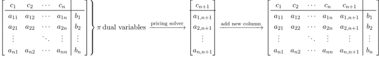
2.6 Column generation

Column generation is a famous technique for solving LPs with large number of variables. The core of the method is not to consider all the variable configurations at once, but rather

(36)

start with small number of them and generate the new ones on the fly as it is needed in order to improve objective value. The point is that one can prove that all the variables presented in a model are not needed for finding and proving optimal solution but specific subset of them is just enough (Desrosiers and L¨ubbecke, 2005).

The obvious question could arise, how one can possibly know which new variable should be generated at the given step? The answer lies in the dual formulation of the given problem — find the constraint in the dual problem which corresponds to variable we wish to generate in master problem and find cutting plane in that form such that it will make current dual solution infeasible. This gives us a new variable for the primal program (see Figure 2.5). Procedure repeats until we are able to find some cuts in the dual problem which violate current dual solution. If there is no such a cut, primal (and also the dual) programs are solved up to the optimality.

Now the question is how to find such cuts. In order to do that, one has to design dedicated algorithm taking into account the form of the dual constraint which we want to be violated. We call this task a subproblem (pricing problem) and the corresponding algorithm a subproblem (pricing) solver. Computational complexity of the subproblem solver is problem-specific. For some problems, we can find polynomial time computable subproblems or pseudopolynomial algorithms (for example incutting stock problem where the subproblem is aknapsack problem

(Korte et al., 2002)). In other cases the complexity can be N P-hard without any known pseudopolynomial algorithm.          c1 c2 · · · cn a11 a12 · · · a1n b1 a21 a22 · · · a2n b2 .. . . .. ... ... an1 an2 · · · ann bn                          

πdual variables−−−−−−−−→pricing solver          cn+1 a1,n+1 a2,n+1 .. . an,n+1         

add new column −−−−−−−−−−→          c1 c2 · · · cn cn+1 a11 a12 · · · a1n a1,n+1 b1 a21 a22 · · · a2n a2,n+1 b2 .. . . .. ... ... ... an1 an2 · · · ann an,n+1 bn         

Figure 2.5: Column generation procedure. It generates a new column that could improve primal objective based on the current dual solution.

Our subproblem is usually viewed as aresource constrained shortest path on acyclic graphs problem. This is identified (Irnich and Desaulniers, 2005, pp. 4) to be inN P-hard complexity class, which is the result consistent with the previous statement that Nurse Rostering Problem is contained withinN P-hard complexity class.

From the LP solver point of view, the column generation procedure is also computation-ally efficient since we can use previous basis as a starting point for the next iteration with additional variables. Therefore, it is not solving the problem every time from scratch.

One has to keep in mind that column generation does not ensure the integer property of the solution. As we said before, it is the solution method for continuous optimization

(37)

problems. In our problem we have to ensure integer property by different mechanism called

branching (see Chapter 4.5).

We offer two different perspectives on the intuition why the column generation works in the following paragraphs below. Then, in the next chapter, we formally derive the column generation procedure for our problem.

Primal perspective Column generation generates variables (columns in Simplex tableau) for the primal program. This step cannot increase the objective value since we can always set the new variable yil to zero in order to obtain previous solution which is also feasible in the

modified problem. Moreover, selecting (even part of) this variable can decrease the objective value because it could fulfill the coverage constraints (2.23) better.

Dual perspective In the dual task (2.34) we are adding (the most) violated constraints in current dual solution into the model. To see why it is needed, one needs to consider the

weak duality theorem (Boyd and Vandenberghe, 2004) which states that the objective value of the dual will be always less or equal to the primal objective value (i.e. the dual is a lower bound on the primal). Since we are restricting polyhedron over which the maximization is performed, the dual objective remains equal or decreases. This will weaken a lower bound on the primal objective which consequently can be decreased by the solver. Essentially, we are trying to cut out the optimal dual feasibility polyhedron which corresponds to the optimal set of variables in primal. See Figures 2.6a and 2.6b for the visualization.

(38)

2 BRANCH AND PRICE METHOD -2 -1 0 1 2 -2 -1 0 1 2 -2 -1 0 1 2 -2 -1 0 1 2 -2 -1 0 1 2 -2 -1 0 1 2 0 20 40 60 80 100 primal dual

(a)Current dual solution

0 20 40 60 80 100 dual primal

(b) Making dual solution infeasible

Figure 2.6:Optimization in dual space over 3 variables. Displayed polytope is a feasible region of dual LP. Inserting a cutting plane (a new schedule) (see Figure 2.6b) makes current dual solution infeasible, thus it lowers the dual objective value and consequently reduces the primal objective.

2.6.1 Derivation

In order to make current dual solution infeasible, one has to find a cut, which will be violated. We have constraints in form of (2.38) in the dual formulation of the master problem. There is an exponential number of them, however, just a subset of them is active in the optimum. One has to solve a problem of findingail in order to find cuts from this set which

are violated γi+ X m∈M X j∈J X k∈K ailmjkπmjk> cil (2.43)

Obviously, it is equivalent to solving 0> cil−γi− X m∈M X j∈J X k∈K ailmjkπmjk =µi (2.44)

(39)

The expression on right-hand-side of (2.44) is called the reduced cost, thus we say that we are looking for columns with negative reduced cost (µi <0). The cil is the cost of pattern l

under a working contract and shift preferences of employeei. It can be rewritten in terms of original variables as cil(x) = X p∈Pi clb_p max{0, lbp−#p}+cubp max{0,#p−ubp}+ X m∈M X k∈K pimkxmk (2.45)

wherepimk is a penalty for not assigning shiftkon daymto employeei,Pi is a set of patterns

for employeei, #p is number of matches of patternp in schedulexand clb

p (cubp ) is a penalty

for violation #p of boundlbp (ubp respectively).

2.7 Algorithmic description

For complete description of the algorithm see pseudocode Algorithm 1. Algorithm 1:Branch and price

1 initColumns, U B←heuristics() 2 queue←RM P(initColumns) 3 whilequeue is not empty do 4 RM P ←queue 5 do 6 solution←solve(RM P) 7 yil ←pricing(RM P) 8 if lb(RMP) >UB then 9 go to 3. 10 end

11 add columny_il into theRM P

12 while column with negative reduced cost exists; 13 if solution is integer-valued then

14 if obj < UB then 15 U B ←obj 16 end 17 else 18 if obj ≤ UB then 19 queue←branch(RM P) 20 end 21 end 22 end

(40)

Individual parts of the branch and price algorithm are described in the following pages: heuristics is described in Chapter 4.2 , solve in Chapter 4, pricing in Chapter 3, lb in Chapter 4.4 andbranch in Chapter 4.5.

(41)

3 PRICING PROBLEM

3 Pricing problem

Pricing problem provides new columns which are candidates for entering the Simplex basis and, thus, decreasing the primal objective value. In our case, the pricing problem represents N P-hard problem which has to be solved repeatedly. Since it is used frequently in the branch and price algorithm, its runtime must be as low as possible. In following sections we show different methods for solving it and ways for speeding it up.

This chapter is organized as follows: first, in Chapter 3.1 we formally define the pricing problem, then in Chapter 3.3 we will show different solution methods we have developed, in Chapter 3.4 we will show how the exact pricing method can be turned into an effective heuristics and in Chapters 3.5 through 3.7 we conclude with some theoretical properties of the pricing problem.

3.1 Definition

The pricing problem is given by the following mathematical programming model min x −γi− X m∈M X k∈K πmkxmk+cil(x) (3.1) subject to ∀m∈ M: X k∈K xmk = 1 (3.2) x∈ {0,1}|M|×|K| (3.3)

wherex are original variables (assigning days to the shifts), γi and πmk are constants in R andcil is defined as in (2.45).

The description of the equation (2.45) mentions term number of matching frequently. One way how to understand it is to treat the employee’s schedule as a finite word from the alphabet K. A matching refers to whether it is contained in regular language defined by a regular expression representing the pattern (see Figure 3.1). Sometimes the pattern is matched multiple times in the schedule, so we sum up occurrences.

· · · − E E − N D · · ·

| {z }

pattern”(E or D), Off, N” is matched Figure 3.1: An example of a pattern matching in a schedule.

(42)

3 PRICING PROBLEM

Due to historical reasons the pricing problem in Nurse Rostering — searching for a schedule for individual employee — is often described as aresource constrained shortest path problem (Irnich and Desaulniers, 2005) (see Figure 3.2). The reason is that in the past, most of the approaches did not consider patterns as soft constraints (Burke et al., 2004), therefore, a certain number of appearances of such pattern in a schedule was consider as resource on the path, which was limited (hence the wordconstrained).

S N1 D1 Off1 N2 D2 Off2 N3 D3 Off3 N4 D4 Off4 T

Figure 3.2:Graph structure for the pricing problem. Vertical layers correspond to days and vertices to shift types. We are interested in finding the cheapests−tpath which satisfies given constraints.

However, the modern treatment of Nurse Rostering Problem (see Chapter 1.1) has only a little connection with previous point of view. We consider number of pattern matching in the schedule as a soft constraint, thus we cannot cut off this ”path” in a simple way and therefore, it makes only a little sense to imagine them as paths.

In fact, soft constraints are not constraints in a sense that they would restrict the set feasible solutions. They are actually changing the objective function of the problem. If a soft constraint is ”violated”, it adds a penalty to the objective. Therefore, every soft constraint is actually presented in the objective in some way. Essentially, there are no constraints in our pricing problem, just a complex, non-convex objective function spanning across a space of schedules, which is given byK|M|_{. Moreover, the objective function changes during iterations}

of column generation. Since we consider very general form of patterns defining quality of a schedule, there is no obvious way how to prune the search space.

These properties of the problem hints to the branch and bound based solution method. Fortunately, we were able to derive a strong lower bound based on the linear programming relaxation (see Chapter 3.5) which helps significantly to speed up the algorithm. It makes it very fast in practice and furthermore it allows to control the quality of solutions produced by the pricing algorithm (see Chapter 3.4.1).

(43)

3 PRICING PROBLEM

random ones but rather tend to have some reasonable structure (it is unlikely that individ-ual schedules in optimal roster will contain shift assignments scattered randomly across the planning horizon) we can derive some properties of the objective function automatically by machine learning algorithms and apply gained knowledge throughout the solution process (see Chapter 5.2).

3.2 Computational complexity

Most of papers argue about the complexity of Nurse Rostering Problem by stating that for a single employee it is a resource constrained shortest path (RCSP) problem whose complexity is N P-hard as shown in (Irnich and Desaulniers, 2005). However, we were not able to find formal proof of the reduction of the pricing problem with soft constraints to the RCSP. Thus, we will show what is the complexity of decision version of our pricing problem below.

Proposition Determining whether the column with negative reduced cost exists is N P -complete.

Proof We show that 3-SAT3 is polynomially reducible to the Pricing Problem. For each instance of 3-SAT we show how to define an instance of pricing problem such that given 3-SAT instance is satisfiable if and only if the given instance of pricing problem (i.e. column) has a negative reduced cost.

Suppose we have a 3-SAT instance with n literals and m clauses. We define a pricing instance with length of planning horizonnwith 2 shift types (e.g.− andD). We set

∀m∈ {1. . . n},∀k∈ {−, D}: πmk := 0

γi := −0.5

For each clause p we define a match with lower bound lbp := 1 and upper bound ubp := 3

with costsclb_p =cub_p := 1. Each match has exactly 3 patterns to be matched — for each literal xi in clausep we add a patternDwith starting day iand for literals in negative sense¬xj a

pattern−with starting dayj. This reduction is clearly polynomial.

Now we show the problem equivalence. Suppose we have a satisfiable formula in 3-CNF. Therefore, at least one literal in each clause p must be true. Since it holds, corresponding pattern will be matched, thus the lower bound of the match lbp will not be violated. When

we consider the definition of the soft cost penalties of the pricing problem (2.45), it is easy

(44)

3 PRICING PROBLEM

to see that there exists a column with reduced cost−0.5, i.e. it is the negative one. In other way around, suppose that a column with negative cost exists. Since this will only happen when there are no soft constraints violated (at least one pattern is matched in each match), it implies that every clause of the 3-CNF formula is true, i.e. the formula is satisfiable.

Up to this we showed that 3-SAT.p Pricing Problem. Now we show that Pricing Problem

is contained inN P which concludes the proof. This is easy to see, since we have p matches where each of them can be evaluated in constant time. Sincepis polynomial innwe compute reduced cost in polynomial time and compare it with 0.

Proposition Pricing Problem is not polynomially approximable within > 0 unless P = N P.

Proof Using reduction of 3-SAT problem to the Pricing Problem shown above we will show that MAX 3-SAT4 Problem polynomially reduces directly to the Pricing Problem. We con-struct an instance of the Pricing Problem such that number of unsatisfied lower bounds on pattern matches is minimized. Since MAX 3-SAT is not polynomially approximable within (Pardalos and Xue, 1994) we conclude that Pricing Problem cannot be polynomially arbi-trarily approximated also.

3.3 Exact solution methods

Having an exact solution method for pricing problem is necessary — at some stage algo-rithm has to prove that restricted master problem converged, i.e. no column with negative reduced cost exists (see diagram in Figure 2.1). As we proved above, this task isN P-complete, thus it is hard to solve it in reasonable time like we demand.

3.3.1 Branch and bound with domination rules

We have designed an exact algorithm based on branch and bound method with dominance rules on partial solutions. It prunes nodes in the search tree (i.e. partial solutions) not only based on lower and upper bounds but also by reasoning about their structure.

For each partial solution it keeps track on the number of matching of each pattern and lower bound on its objective value. Based on the structure of patterns, one is able to reason

4

It is the problem where we want to maximize the number of satisfied clauses in given 3-CNF propositional logical formula.

(45)

3 PRICING PROBLEM

whenever for given two partial solutions of the same length one dominates other (i.e. its objective cannot be worse than the other) or if they are incomparable. When one of the partial solutions is dominated by another one, we can prune whole subtree of that solution (see Figure 3.3). The efficiency of the algorithm depends on the power of the domination technique.

E

EE ED EN

EEE EED EEN EDE EDD EDN END ENN ENE

ENEE EENE

Figure 3.3: An illustrative example of the search tree with some dominated partial solutions. Consider a constraint where we want to have at least two Eshifts in schedule. Partial scheduleEDDis dominated byEEN,

EDNis dominated byENE.

However, since we are mostly dealing with soft constraints, design of such procedure is not trivial. We were able to develop following method.

Dominance rule Our dominance procedure compares two partial solutions of the same length. The domination is resolved based on the number of matches of each pattern. We divide patterns into two groups and patterns from each group are treated from two different perspectives — constraint on minimal and constraint on maximal matching. We frequently use the fact that number of pattern matches is non-decreasing. This is easy to see since adding a new shift to the end of the partial schedule cannot undo the pattern match done before, therefore it can only stay the same or increase.

N E − N · · · π1−: 0 π3−: 0 π3−: 0 π4−: 0 · · · π1E: +100 π2E: -100 π3E: +100 π4E: +100 · · · π1D: +100 π2D: -100 π3D: -100 π4D: +100 · · · π1N: -100 π2N: +100 π3N: +100 π4N: 0 · · · Constraints: a) Min 1 D, Max 3 D b) Max 1 NE

Figure 3.4: An illustrative example of resources. Partial solution NE-N is associated with resource vector [−200,0,1]. The first element is associated with the partially evaluated reduced cost, the other are resources associated with constraints a) and b). Dominance procedure compares vectors of corresponding partial solutions element by element.

(46)

3 PRICING PROBLEM

setP_i by a lower bound on its reduced cost. We refer to each of those numbers as a resource. A resource in partial solution ais denoted #a (see example in Figure 3.4).

As we said, patterns are divided into two groups. The first group contains patterns with unit length and the second one contains patterns spanning across more days. We define dominance on separate resources as follows:

1. lower value of the lower bound on the reduced cost dominates the higher one 2. for patterns of unit length

(a) minimum matching:

i. if #a< lb and #b < lb then the solution with higher # dominates the other

ii. if #a< lb and #b ≥lb thenb dominatesa

iii. if #a≥lb and #b ≥lb thenequivalent

(b) maximum matching:

i. if #a≤ub and #b ≤ub then the solution with lower # dominates the other

ii. if #a≤ub and #b > ubthenadominates b

iii. if #a> uband #b > ubthen the solution with lower # dominates the other

3. for longer patterns

Even though patterns of unit length are a special case of longer ones, we treat them separately due to following notion of future matching. We can reason about patterns with length greater than 1 based on the possibility they will match on current ending of the partial solution. Suppose a pattern of length k and denote ∀i ∈ {1. . . k −1} possibilities of overlapping the pattern with the ending of partial solution aas #Ma(i).

Then

(a) minimum matching:

i. if #a≥lb and #b ≥lb thenequivalent

ii. else if #a< lb and #b ≥lb thenb dominatesa

iii. else

A. if∃i, j : #Ma(i) >#M_b(i) and #Ma(j) <#M_b(j) then aand b are incompa-rable

B. if∀i: #Ma(i)≥#M_b(i) and ∃j: #Ma(j)>#M_b(j) thenadominatesb

C. else equivalent

(b) maximum matching: