MITSUBISHI ELECTRIC RESEARCH LABORATORIES http://www.merl.com
Boosting Adaptive Linear Weak Classifiers
for Online Learning and Tracking
Toufiq Parag, Fatih Porikli, Ahmed Elgammal
TR2008-065 October 2008
Abstract
Online boosting methods have recently been used successfully for tracking, background sub-traction etc. Conventional online boosting algorithms emphasize on interchanging new weak classifiers/features to adapt with the change over time. We are proposing a new online boosting algorithm where the form of the weak classifiers themselves are modified to cope with scene changes. Instead of replacement, the parameters of the weak classifiers are altered in accordance with the new data subset presented to the online boosting process at each time step. Thus we may avoid altogether the issue of how many weak classifiers to be replaced to capture the change in the data or which efficient search algorithm to use for a fast retrieval of weak classifiers. A computationally efficient method has been used in this paper for the adaptation of linear weak classifiers. The proposed algorithm has been implemented to be used both as an online learning and a tracking method. We show quantitative and qualitative results on both UCI datasets and several video sequences to demonstrate improved performance of our algorithm.
CVPR 2008
This work may not be copied or reproduced in whole or in part for any commercial purpose. Permission to copy in whole or in part without payment of fee is granted for nonprofit educational and research purposes provided that all such whole or partial copies include the following: a notice that such copying is by permission of Mitsubishi Electric Research Laboratories, Inc.; an acknowledgment of the authors and individual contributions to the work; and all applicable portions of the copyright notice. Copying, reproduction, or republishing for any other purpose shall require a license with payment of fee to Mitsubishi Electric Research Laboratories, Inc. All rights reserved.
Copyright cMitsubishi Electric Research Laboratories, Inc., 2008 201 Broadway, Cambridge, Massachusetts 02139
Boosting Adaptive Linear Weak Classifiers for Online learning and Tracking
Toufiq Parag
Dept of Computer Science
Rutgers University
Piscataway, NJ 08854
Fatih Porikli
Mitsubishi Electric Research Labs
Cambridge, MA 02139
Ahmed Elgammal
Dept of Computer Science
Rutgers University
Piscataway, NJ 08854
Abstract
Online boosting methods have recently been used suc-cessfully for tracking, background subtraction etc. Conven-tional online boosting algorithms emphasize on interchang-ing new weak classifiers/features to adapt with the change over time. We are proposing a new online boosting algo-rithm where the form of the weak classifiers themselves are modified to cope with scene changes. Instead of replace-ment, the parameters of the weak classifiers are altered in accordance with the new data subset presented to the on-line boosting process at each time step. Thus we may avoid altogether the issue of how many weak classifiers to be re-placed to capture the change in the data or which efficient search algorithm to use for a fast retrieval of weak classi-fiers. A computationally efficient method has been used in this paper for the adaptation of linear weak classifiers. The proposed algorithm has been implemented to be used both as an online learning and a tracking method. We show quan-titative and qualitative results on both UCI datasets and sev-eral video sequences to demonstrate improved performance of our algorithm.
1. Introduction
Studies on online learning algorithms originated in com-putational learning community. The initial algorithms train several experts based on the labeled samples arriving se-quentially and later combine the predictions of these experts to categorize any new example. The algorithms popular to the machine learning researchers like the weighted majority algorithm or winnow algorithm, as discussed by Littlestone and Warmuth in [11] and by Littlestone in [10] respectively, belong to this family1. Both the weighted majority and
win-now algorithms works as a committee of hypotheses to clas-sify target samples. The popular (offline) Adaboost classi-fier [7] resembles these classifiers in the sense that it also 1A more detailed discussion on online learning algorithms is provided by Blum in [3]
combines several ‘weak’hypotheses in classifying new ob-servations. An online version of the boosting classifiers in has been recently proposed in a relatively recent study by Oza et.al [12].
Online learning algorithms can be immediately applied to the object tracking scenario. The tracker employs an on-line learning method to learn the object from frames arriv-ing sequentially and then apply the classifier to detect the target in the next frame. Recently, the work of Avidan [2] and Grabner et.al. [8] has shown impressive results of us-ing classifier based trackus-ing methods. The classifier based methods initially learn a binary classifier to distinguish the object of interest from the (neighboring) background and then apply it at each new frame to locate the position of the object. Both the works of [2] and [8] uses AdaBoost [7] or an online variant of AdaBoost classifier.
Several previous works have addressed object tracking problem by approximating the distribution of feature re-sponses representing an object using Kalman Filter [6], Par-ticle Filter [9], Mean-shift method [5] etc. Density approx-imation tracking algorithms result in inferior performances to classifier based tracking algorithms in the cases when the target appearance undergoes substantial change over time or when there are similar objects nearby [2]. Results of our experiments will show how the proposed method is able to track objects in such scenarios where meanshift tracker fails.
One important issue to resolve in classifier based track-ers is how to adapt with scene change and remain capa-ble of identifying the object correctly. We should keep in mind that both the background and the object of interest may change with time. The previous studies [2,8] replace a subset of current weak classifiers with a new one to cope with scene changes. Ensemble tracking [2] does not up-date the weak classifiers themselves. Instead at every frame, it replaces some of the older weak classifiers with several new weak classifiers. Grabner’s online boosting method [8] models the feature densities by simple Gaussians and up-date their parameters at each frame using Kalman filtering method. Even if we assume that a Gaussian distribution is
sufficient to model feature densities (which is usually not the case), the updating mechanism soon becomes compli-cated and slow if we wish to use higher dimensional weak classifiers. Furthermore, the method of [8] immediately throws away any weak classifier generating an error greater than or equal to 50%. To fill up the space evacuated by the leaving weak classifier, the methods in both [2] and [8] have to search a large subset of weak classifiers for replacement.
Theprimary contributionof this paper is an adaptation
scheme for the weak classifiers themselves to conform with the changes over time. Similar to the method of ensemble tracking [2], we combine linear weak classifiers, learned in a least square fashion, and learn incrementally (online boosting). However, we neither replace weak classifiers for each data set nor do we throw out any weak classifier during training phase. Instead, the proposed method modifies the internal parameters of the base learners for the final clas-sifier to blend with the change as long as the base learner has an error rate below 50%. The online boosting algo-rithm described in this paper uses linear regressors as the base learners. The adaptation scheme does not require us to keep the previous examples in the memory and does not need complex filtering techniques. This paper also demon-strates how the adaptation process can also ‘forget’previous observations.
In the previous studies of online boosting that [2,8], it has not been guaranteed that, interchanging a fixed num-ber of weak classifiers will be able to identify and capture the change in pattern induced by new samples. Therefore, the number of weak classifiers to be replaced is an exter-nal parameter to these methods and the choice of such pa-rameter is still unresolved. Furthermore, the time complex-ity of these methods will also increase with the increase in the number of base learners to be replaced. The proposed method, instead of replacement, keeps modifying the form of as many hypotheses as necessary to adapt to any new trend in the dataset. Therefore, the proposed method is ca-pable of identifying the object with substantial change in the appearance during tracking. We show results where our algorithm supersedes previous method of tracking for track-ing such objects in the results section. Our method also pro-duces comparable performance w.r.t. its offline counterpart in classifying the UCI data.
The paper is organized as follows. We start with describ-ing offline and online boostdescrib-ing algorithms in sections 2.1
and2.2respectively. sections3 and4illustrates the least square fitting of linear regressors, how to modify them to cope with new data and how to incorporate these linear functions into online boosting. With a brief description of how to apply online boosting for object tracking in sec-tion5, section6analyzes the performance of the proposed algorithm. Finally, we summarize our findings in Section7.
2. Background and Related Work
2.1. Offiline Boosting
Boosting was proposed as a classification algorithm in [7]. Any input x ∈ RL is categorized as one of the
classes 1 or -1 using the sign of the function H(x). The function H : RL → {−1,1}, also known as the strong
classifier, is a linear combination of several other functions
fk(x), k= 1,2,· · ·K. H(x) = sign XK k=1 ckfk(x) . (1)
The functionsf(x) : RL → {−1,1}, known as the base
learners or weak classifiers in the boosting literature, are also classifier functions except (as their name implies) they do not possess a high rate of accuracy. It has been proved in [7] that, even if the individual performances of the weak learners are barely satisfactory (error rate > 50%), their combination could be highly effective in terms of error.
The AdaBoost classifier is trained in an iterative fashion on the whole datasetX˜ ∈ RN×(L) and their
correspond-ing labels y˜ ∈ {−1,1}N. First, each of the samples are
imposed a uniform boosting weightw0
i = N1 andw0 =
[w0
i]Ni=1such that
P
iwi = 1.Then, atk-th step the the
al-gorithm searches the f(x)producing the lowest expected error w.r.t. the boosting weights w. The mixing weight for the linear combination given in Eqn1is calculated by
ck = 1 2log1−²
k
²k . In the next iteration of boosting, the
weights are modified bywk+1
i = w
k
iexp(ckyifk(xi))
Zk so that
the examples missed by fk(x) receives a higher weight.
The weights are then normalized by Zk to maintainw as
a probability vector. In the following description, we will omit the the superscripts ofwkandf(x)unless when they
seem essential for precise description.
2.2. Online boosting
The underlying idea for development of online boosting classifier is to learn incrementally. We wish to build the classifier in an environment where the samples arrive one after another as opposed to batch learning, where the whole dataset is available to learn from. The work by Oza et. al. [12] models the sequential arrival of samples by a Pois-son distribution. Each of the weak classifiers of the pool is learned and updated on each sample k times in a row wherekis a random number generated by Poisson(λ). If any example is misclassified by a base learner, the Poisson parameter (λ) increases. Therefore, the next base learner will concentrate more on learning the misclassified sample due to a large value ofk. The value of Poisson parameterλ
is also accumulated to calculate the mixing weights of the hypotheses (e.g.ckin Eqn1).
However, Oza et.al. did not discuss much about how to update these weak hypotheses. Grabner et. al. [8] in-troduced online boosting algorithm to the vision commu-nity and showed results on different problems. To update the weak hypotheses, the authors of [8] proposes to incre-mentally model the sample distribution with the help of a Kalman filter [13]. Their implementation also replaces a set of weak classifiers with a new one. Replacing a set of base learners with a new set has also been proposed by Avidan [2]. Avidan’s work was primarily concentrated on tracking using a boosting method that adapts to the change in scenes by adding new members and removing the old ones from the weak classifier pool. In this work, we only update the linear weak classifiers (learned in a Least Square method) to cope with the new data samples. The following subsections describe the update procedure of weak classi-fiers and how they are incorporated in boosting framework.
3. Adaptive Linear Weak Classifier
3.1. Weighted Linear Regressor
Let us supposeX ∈RN×(L+1)is the data matrix where
there areN observationsx∈RL(the last column ofXis a
vector of all ones that is used for calculating the intercept). The corresponding labels for these examples are stored in
y ∈ {−1,1}N. To solve a linear relation Xβˆ = y by
least squares method, we have to minimize the error func-tion(y−Xβˆ)T(y−Xβˆ). If the different samples have
different importance weights quantified by the vectorw, as they do in AdaBoost, we have to minimize the error func-tion(y−Xβ)TW(y−Xβ)whereWis a diagonal matrix
withwon its diagonal. The linear coefficientsβthat mini-mizes the error is given by the following expression.
β= (XTW X)−1XTWy. (2) Denoting the quantities XTW X, XTWy as P ∈ RL+1×L+1ands∈RL+1respectively, the expression can
be abbreviated asβ=P−1s.The base learners we used in
this study are linear classifiersf(x) :RL → {−1,1}. The
response off(x)is calculated as follows:
f(x) =
1, if [xT 1]β>0;
−1, otherwise. (3)
3.2. Adaptive Linear Regressor
As we mentioned earlier, our weak learners recalculate their parameter values for each new data subset. Let Xτ
denote the examples seen so far up to frametandβτ
de-note the parameters (linear coefficients) of the regressor we learned from Xτ. Then, for a new subset Xν, the new
value of the linear coefficientsβτ+1should be learned on Xτ+1 = [XτT XνT]T andyτ+1 = [yTτ yTν]T by the linear
regression . βτ+1=P −1 τ+1sτ+1. (4) Here, Pτ+1 = XτT+1Wτ+1Xτ+1, sτ+1 = XT τ+1Wτ+1yτ+1, Wτ+1 = Wτ 0 0 Wν where Wν
is a diagonal matrix having the boosting weights on the new sampleswν on its diagonal. It can be easily verified
that, sinceXτ+1 = [XτT XνT]T andyτ+1 = [yτT yTν]T,
the two quantities required for computing βτ+1 can be decomposed and expressed as a recursive summation of previous and new samples:
Pτ+1 = XτTWτXτ+XνTWνXν=Pτ+Pν
sτ+1 = XτTWτyτ+XνTWνyν=sτ+sν. (5) We are describing in the next section how to calculatePτ+1
andsτ+1without storing all the previous examples seen so
far.
3.3. Weak Classifier Memory
Based on the decomposition provided in the previous section, to update the parameterβτ+1, we only need to store a matrix and a vector of sizesL+ 1×L+ 1andL+ 1 re-spectively and compute the two quantitiesPν,sν only for
the new samples. The simplistic form of Eqn5suggests that we can also discard the quantities (i.e. ‘forget’ them) relat-ing to very old examples if we wish to restrict ourselves to only the recent changes. So after the algorithm received a specific number of datapoints, the update equation changes to the following:
Pτ+1 = Pτ+Pν−Pτ−ω
sτ+1 = sτ+sν−sτ−ω. (6) The value of ω decides for how long do we wish to ‘remember’ the contribution of any datapoint to our method. Obviously, we need to store all the quantities
Pτ, Pτ−1,· · ·, Pτ−ω and sτ,sτ−1,· · ·,sτ−ω in a queue.
Since the dimensionality L of the data is usually much smaller than the number of samplesNν in the new set, the
space complexity for this queue is not high.
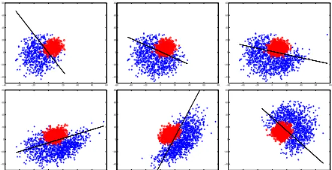
−60 −40 −20 0 20 40 60 80 −40 −20 0 20 40 60 80 −60 −40 −20 0 20 40 60 80 −40 −20 0 20 40 60 80 −60 −40 −20 0 20 40 60 80 −40 −20 0 20 40 60 80 −60 −40 −20 0 20 40 60 80 −40 −20 0 20 40 60 80 −60 −40 −20 0 20 40 60 80 −40 −20 0 20 40 60 80 −60 −40 −20 0 20 40 60 80 −40 −20 0 20 40 60 80
Figure 1. Adaptation of linear classifier. Top row: without forget-ting, bottom row: with forgetting.
To visualize how this adaptation scheme works on any linear classifier, we generated synthetic two-class dataset. As Figure1shows, the blue dots and red circles represent
positive and negative examples respectively. The black line is the classifier learned by the proposed method with uni-form weights (W =I). In the first three image of top row, we are incrementally adding new samples to the dataset and learning the weak classifier according to the update equa-tion 5 without forgetting. In three images of the bottom row, we are also removing the oldest subset and training the linear classifier by the update equation6with forget mech-anism. It can be easily observed how the linear classifier is correctly following the changing pattern of the dataset.
3.4. Temporal weighting
According to the update equation5, all the new samples have equal importance and hence have the same contribu-tion towards the modificacontribu-tion ofβ.Therefore, after several time steps, the weak learner will become biased to the re-cent samples and contributions of the first set of examples will be gradually lost. As a result, the resulting classifier will be unable to classify observations similar to the first ones. Therefore, in this paper, we scaled the quantities used in equation 5with respect to time.
This study uses a temporal weightρτ (decreasing with
time) on the quantitiesPτandsτso that the updated values
of them becomes a weighted cumulative sum.
Pτ+1 = Pτ+ρτ Pν
sτ+1 = sτ+ρτsν (7) The values ofρτ are predefined and decreases withτ. In
our implementation we used ρτ = exp(−τ /σ) whereσ
is a predefined constant. In case of the ‘forgetting’,Pτ−ω
andsτ−ωhave to be multiplied by their respective temporal
weights before being subtracted in Eqn6. But then, all the
Pandsin the queue need to be re-weighted so thatPτ−ω+1
receives the largest weight followed by that ofPτ−ω+2and
so on. Therefore, the new values ofPandsbecomes
Pτ+1 = Pτ−ρ1Pτ−ω+ ωX−1 l=1 ρlPτ−ω+l+ρωPν sτ+1 = sτ−ρ1sτ−ω+ ωX−1 l=1 ρlsτ−ω+l+ρωsν (8) The effect of temporal weights on online boosting will be revisited in section4.
4. Combining adaptive linear regressors for
online boosting
Similar to the previous studies [12,8], we apply the Ad-aboost training algorithm (modified) on every new subset of dataXν.All samples inXν are assigned uniform weights.
For each new subsetXνof data and their labelsyν, we
cal-culate the updated value ofβjτ+1(using Eqn7or Eqn8 de-pending on whether or not we wish to forget) ofj-th weak
hypothesisfj(x)to determine whichfj(x)can most
suit-ably conform itself with the changes. This base learner is immediately included in the strong classifier and the boost-ing weightsware updated accordingly. For rest of the hy-pothesis,βτis not updated toβτ+1until they are found to
be the one generating minimum error w.r.twνand included
in the strong classifier.
We also added some modifications to the original boost-ing method to incorporate the adaptive linear regressors as the weak learners for online boosting. The following para-graphs will describe these changes to Adaboost.
Need-based inclusion of base learners:We start the learn-ing process withKbase learners. The initial data subset is used to train few of theKavailable base classifiers until all samples are adequately learned. We claim that, when the sum of boosting weightswν of the new samples decreases
below a threshold, the examples need not be learned by any-more hypothesis . So, we stop training new weak learners when total weight is below a specific value and the remain-ing of the base learners remain dormant in the pool of weak classifiers. The same strategy has been followed for conse-quent datasetsXνand their labelsyν. Atk= 1, instead of
updating the linear base classifiers, first we apply them on the samples inXν to determine if any of the present
learn-ers can already classify them accurately or not. The update equation is enforced only when the minimum classification error with the current set of learners is not zero and there-fore, the importance weight is significantly large.
Updating Boosting weights w: Every example receives the weight w0
i = 1, i = 1,2,· · ·N initially in our
al-gorithm. We update the weights of the weak classifiers based on the performance of the weak classifier chosen in the latest iteration. But, if we normalize the importance weights after a perfectly correct classification (all samples were classified accurately),wi, i= 1,2,· · ·, Nνwill retain
their previous values and their sum will not fall below the specified threshold. Therefore, the proposed online boost-ing method does not normalize the importance weight after updating.
Effect of temporal weighting:It may appear to the reader that, since we are using a temporal weight decreasing with time, after several time step the new datapoints would not have any influence on the boosting algorithm. To compre-hend why that does not happen, it is important to understand an important fact that not every classifier has a chance to observe each of the samples. This is due to the fact that, we stop training weak learners wheneverwT
ν 1decreases
below a specific threshold. Therefore, the new subset ar-riving at timet = 10may not be theτ = 10th subset that
fj(x)(where 1 ≤ j ≤ K)experienced. Recall that, we
are decreasing the value ofρaccording to the valueτwhich denotes the number of subset the corresponding weak clas-sifier has actually learned on.
OnlineBoost
For each subsetset of new dataXνand their labelsyν
1. Start with uniform distributionwνanddontLearn= 1.
2. fork= 1,2,· · ·K
(a) ifdontLearn= 0then WeakLearn(wν).
(b) errj= CalcResp(fj, X ν).
(c) fk=fj∗wherej∗= arg min
j errj. (d) ck=1 2log1−err j∗ errj∗ (e) ∀wi∈wν wi=wi∗exp(−ckyifk(xi)). (f) ifwT ν1< wththendontLearn= 1.
(g) iferrk>0.5ignoreXν,yνand return.
WeakLearn(wν)
1. Compute new quantitiesPτ+1andsτ+1.
2. Learnβτ+1according to Equation7or Equation8.
CalcResp(fj, X
ν,wν) returnserrj
1. λjcorr=λjcorr+Piwiδ(fj(xi), yi)and
λjmiss=λjmiss+Piwi(1−δ(fj(xi), yi)) wherexi∈Xν, yi∈yνandwi∈wν. 2. errj= λjmiss λjcorr+λjmiss . 3. cj=1 2log 1−errj errj .
Note: Here1is a vector of all ones andδ(a, b) = 1whena= band
δ(a, b) = 0otherwise.
Table 1. Algorithm: Boosting with Linear Adaptive Classifier.
So, for the subset that was fed to the online boosting al-gorithm at timet, it will be theτ1-th andτ2-th new subset for two hypothesisfj1(x)andfj2(x)respectively.
There-fore, even if for some weak learner the temporal weightρτ1
is very small, for other classifierfj2x, the weightρ
τ2 will
be substantially large. Nonetheless, at some point of time, when the value of τ is large for all the base learners, any new subset will not receive the necessary attention. This is exactly the time when we should start ‘forgetting’to make room for new observations.
Calculatingck : The linear coefficientscj combining the
base learners are determined using the overall performance, that is, the overall classification accuracy (or error) on the whole set of training examples. These quantities are cumu-latively stored intoλj
corr(λjmiss.) whereλjcorraccumulates
the summation of boosting weights of samples correctly (in-correctly) classified. For details on these quantities, please refer to [12]. We need to keep in mind that, when we are ‘forgetting’a subset, their corresponding λj
corr andλjmiss
also need be discarded. The complete algorithm for pro-posed method of boosting adaptive linear weak hypotheses is stated in Table1.
5. Application to tracking
An online learning method can be readily applied for tracking objects in a video. Avidan used a modified ver-sion of AdaBoost[2] for tracking objects in consecutive im-ages. We have closely followed the implementation of [2] to apply our online boosting algorithm for tracking. The tar-get is identified in the first frame by the smallest rectangle Rinnercontaining only the object itself. Then a larger
rect-angleRouteris selected around the inner rectangleRinner
to mark the background pixels. All the pixels inRinnerare
considered as positive examples (i.e. yi = 1) and all the
pixels in rectangleRouterare considered as negative
exam-ples (i.e. yi = −1) for learning. In the next frame, the
boosting classifier is applied on all the pixels inRouterto
generate the responses the strong classifier. A meanshift al-gorithm [4] is applied to determine the new location of our target on this response image (also called the confidence map). Once the meanshift algorithm converges, two new rectanglesRinnerandRouterare redrawn around the new
location to label the pixels and the strong classifier is re-trained using the new data subset and their labels.
6. Experiments and Results
6.1. Synthetic data
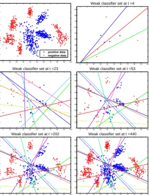
The 2D synthetic data ofN = 440samples was gener-ated from a mixture of Gaussians as shown in the top-left image of Figure 2. The blue ‘*’and red ‘+’s denote the positive and negative examples respectively. We passed a pair of positive and negative examples to the proposed on-line boosting algorithm at a time. Since we do not wish to forget any observations, weak learner memory is not used. The learned classifier was tested on another test dataset gen-erated from the same mixture of Gaussians.
Fig2visualizes how the weak classifiers are being gen-erated and modified according to the changes on these syn-thetic dataset. We are using only K = 10 base learners for this illustration. Each hypothesis correspond to a line in Fig2. Initially, witht < 20, the algorithm tends to gen-erate new weak classifiers and add them to strong classifier to learn the new examples (top row of Fig2). Then, when there are no more hypothesis left unused, the base learners start adapting to the changes (as can be seen in 2nd row of Fig2). Once the algorithm received sufficient samples, the set of weak classifiers are stabilized and remains almost unchanged till we finish learning (last row). One can eas-ily notice how the the converged forms of the classifier are separating the boundaries of two classes.
To compare the performance of the online boosting method, we generated the classification error on the same dataset produced by an off-line Adaboost algorithm with logistic function as the base learner. We used the AdaBoost
0 10 20 30 40 50 60 70 80 90 100 0 10 20 30 40 50 60 70 80 90 positive data negative data 0 10 20 30 40 50 60 70 80 90 100 0 10 20 30 40 50 60 70 80 90
Weak classifier set at t =4
0 10 20 30 40 50 60 70 80 90 100 0 10 20 30 40 50 60 70 80 90
Weak classifier set at t =23
0 10 20 30 40 50 60 70 80 90 100 0 10 20 30 40 50 60 70 80 90
Weak classifier set at t =53
0 10 20 30 40 50 60 70 80 90 100 0 10 20 30 40 50 60 70 80 90
Weak classifier set at t =202
0 10 20 30 40 50 60 70 80 90 100 0 10 20 30 40 50 60 70 80 90
Weak classifier set at t =440
Figure 2. Synthetic 2D data (top-left image) and gradual adapta-tion of weak classifier at timest= 4,23,53,202,440.
implementation of machine learning software Weka [14]. The total number of weak classifier for online and offline boosting was the same. Although we expect any online learning algorithm to exhibit inferior performance to that of its offline counterpart, the proposed algorithm works much better than the offline boosting for this synthetic dataset (as shown in the first row of Table2).
Dataset Training Size of Proposed Offline set test set % correct % correct synthetic 440 + 440 440 + 440 94.43 72.61 ionosphere 75 + 75 150 + 51 84.07 83.08 breast cancer 100 + 100 112+257 90.24 91.32 diabetes 130 + 130 138 + 370 63.18 72.63 spam 500 + 500 1313 + 2288 87.67 89.58
Table 2. Classification rates on synthetic and UCI data
6.2. UCI datasets
We followed the same strategy we used for synthetic data on UCI [1] datasets ‘ionosphere’, ‘breast cancer’, ‘dia-betes’and ‘spam’. First, each of these datasets were sepa-rated into training and testing subsets. Then, training sam-ples were supplied to the learning algorithm in pairs of a positive and a negative example and none of the observa-tions were ‘forgotten’. The results, using both the proposed online boosting method and the offline AdaBoost imple-mentation of Weka on several UCI datasets are given in Table2. Both online and offline boosting classifiers
com-priseK = 30bse learners for all dataset but ‘spam’. Since ‘spam’dataset is considerably larger than others, the total number of base learners used to learn it wasK = 50.The results suggests that we can have competitive performance by online boosting with adaptive linear weak classifiers for real datasets too.
6.3. Tracking examples
For tracking, we processed the images of video follow-ing the procedures used in Avidan’s work [2]. As described in section5, the samples within the inner rectangleRinner
were regarded as positive examples and that withinRouter
were considered as negative examples. In all the following experiments, the features used to represent the pixels were only R, G, B values.
The total number of weak learners used in all the track-ing examples is 8. We fixed a the number of previous frames that we wish to ‘remember’and discarded earlier observa-tions from the data. The queue length for weak learner memory wasω = 15, i.e., the learners ‘forgets’everything happened before 15 frames. The temporal weights are cal-culated with σ = 3. The procedure for outlier detection of [2] was also followed in our implementation. In what follows in this section, we will show some image sequences where the proposed method outperforms the meanshift [4] and ensemble trackers [2] respectively.
Comparison with meanshift:Figures 3 (a), (b) and (c) compare the performance of the proposed online boosting algorithm to a meanshift tracker. Our first dataset (as shown in Figure3) (a) contains images of a police car chase. At a certain stage of chasing, the car being chased (also the ob-ject which we are tracking) completely turns around and then tries to flee again in another direction. We show in Figure3(a) that even though meanshift tracker was able to track the car after the collision, if fails to follow the object due to an occlusion by roadside pole and trees. But, our online learning adapts itself to the changes very rapidly and tracks it correctly. Since the current implementation of our algorithm can not modify the target window according to rotation or scale changes in the object, the target window was not redrawn according to the new appearance of the object.
The second dataset were recorded by a moving camera. In Figure3(b), three vehicles with similar appearances cross each other in the opposite direction. While the meanshift tracker confuses the target truck with the other one, the pro-posed learning algorithm remains capable of distinguish-ing the target. The last comparison (Figure3(c)) manifests how our algorithm adapts with illumination change (notice Frames 38 and 199) whereas meanshift tracker cannot.
Comparison with ensemble tracker:The ensemble track-ing method [2] cope with the change in scene by replac-ing a set of base learners with new ones. The number of
Frame 178 Frame 199 Frame 255 Frame 260 Frame 278 (a) Car chase
Frame 112 Frame 264 Frame 279 Frame 296 Frame 350
(b) Vehicles crossing
Frame 16 Frame 33 Frame 40 Frame 49 Frame 70
(c) Illumination change.
Figure 3. Performance comparison (a), (b) and (c) with meanshift tracker. For each output sequence, top row: meanshift tracker, bottom row: proposed method
weak learners to exchange is an external parameter to the algorithm. We can not expect that replacing any fixed num-ber of weak classifiers can always capture the change with time. This is exactly what happens when ensemble tracker looses the target object in Figures4(a) and (b). In the video of cars on a city street at night (Figure 4(a)), the ensem-ble tracker gets distracted by the rotating red light of the police car and eventually ends up on another car facing in the reverse direction. Since we are modifying all the base learners (if necessary), the online boosting method tracks the object accurately. In Figure4(b), the tracker confuses the tracked person wearing a red jacket with another person wearing similar attire. The output of the proposed learning
method, as shown in the bottom row(s), clearly exhibits the robustness of method for both identification and capturing the changes.
Table3displays number of frames of the aforementioned datasets correctly tracked by the proposed method and other methods. The number of frames were calculated manually from the output images. If in any frame, 25% of the target window does not contain the object (approximately, except CarChase sequence), we classify the frame as being incor-rectly tracked. As we can see, in all the videos where the traditional methods fail, our method can track the target for almost the full length of the sequence.
Frame 5 Frame 73 Frame 174 Frame 259 (a) Police car at night
Frame 5 Frame 12 Frame 17 Frame 22
(b) Person with red jacket
Figure 4. Performance comparison (a) and (b) with ensemble tracker. For each output sequence, top row: ensemble tracker, bottom row: proposed method.
Dataset Object meanshift ensemble Proposed CarChase car 250/285 - 285/285 VehiclesCrossing car 260/395 - 390/395 IlluminationChange person 38/76 - 92/92
PoliceCarNight car - 40/290 280/290 PersonRedJacket person - 10/45 45/45 Table 3. Frames exactly tracked by the proposed & other methods
7. Conclusion
This study proposes a new online boosting by continu-ous updating of weak classifiers. Results on artificial and real datasets shows the better performances achieved for both online learning and object tracking purposes by the proposed method than that of previous methods.
Acknowledgement:This research was partially funded by NSF CAREER award IIS-0546372 and Mitsubishi Electric Research Labs.
References
[1] A. Asuncion and D. Newman. Uci machine learning repository, 2007. UC Irvine, School of ICS.6
[2] S. Avidan. Ensemble tracking. InCVPR, pages 494–501, 2005.1,2,
3,5,6
[3] A. Blum. On-line algorithms in machine learning. Online Algo-rithms: The State of the Art, LNCS 1442, 1998.1
[4] D. Comanciu, R. Visvanathan, and P. Meer. Kernel-based object tracking.TPAMI, 25(5):564–575, 2003.5,6
[5] D. Comaniciu, V. Ramesh, and P. Meer. Real-time tracking of non-rigid objects using mean shift. InCVPR, 2000.1
[6] F. Dellaert and C. Thorpe. Robust car tracking using kalman filtering and bayesian templates. InConference on Intelligent Transportation Systems, 1997.1
[7] Y. Freund and R. E. Schapire. A decision-theoretic generalization of on-line learning and an application to boosting.Journal of Computer and System Sciences, 55(1):119–139, 1997.1,2
[8] H. Grabner and H. Bischof. On-line boosting and vision. InCVPR, pages 260–267, 2006.1,2,3,4
[9] M. Isard and A. Blake. Condensation – conditional density propaga-tion for visual tracking.IJCV, 29(1):5–28, 1998.1
[10] N. Littlestone. Redundant noisy attributes, attribute errors and linear threshold learning using winnow. InFourth Annual Workshop on COLT, pages 147–156. Morgan Kaufmann, 1991.1
[11] N. Littlestone and M. K. Warmuth. The weighted majority algorithm.
Information and Computation, 108(2):212–261, 1994.1
[12] N. Oza and S. Russell. Online bagging and boosting. InArtificial Intelligence and Statistics, pages 105–112, 2001.1,2,4,5 [13] G. Welch and G. Bishop. An introduction to kalman filter, 1995.
Tech Report., Univ of NC-CH, Dept of Computer Science.3 [14] I. H. Witten and E. Frank.Data Mining: Practical machine learning
tools and techniques, 2nd Edition. Morgan Kaufmann, San Fran-cisco, 2005.6