regression models for
longitudinal data with possibly
incomplete sequences
c
The Author(s) 2015 Reprints and permission:
sagepub.co.uk/journalsPermissions.nav DOI: 10.1177/ToBeAssigned www.sagepub.com/
Maria Francesca Marino
1, Nikos Tzavidis
2and Marco Alf `
o
3Abstract
Quantile regression provides a detailed and robust picture of the distribution of a response variable, conditional on a set of observed covariates. Recently, it has be been extended to the analysis of longitudinal continuous outcomes using either time-constant or time-varying random parameters. However, in real-life data, we frequently observe both temporal shocks in the overall trend and individual-specific heterogeneity in model parameters. A benchmark dataset on HIV progression gives a clear example. Here, the evolution of the CD4 log counts exhibits both sudden temporal changes in the overall trend and heterogeneity in the effect of the time since seroconversion on the response dynamics. To accommodate such situations, we propose a quantile regression model where time-varying and time-constant random coefficients are jointly considered. Since observed data may be incomplete due to early drop-out, we also extend the proposed model in a pattern mixture perspective. We assess the performance of the proposals via a large scale simulation study and the analysis of the CD4 count data.
Keywords
Latent Markov models, Missing data, Informative drop-out, Latent drop-out classes, Nonparametric Maximum Likelihood, Mixed models.
1
Introduction
In longitudinal studies, measurements recorded on the same individual are likely correlated. In the “standard” (mean) regression context, within-individual dependence is often accommodated by postulating a conditional model augmented by individual-specific sources of unobserved heterogeneity. Marginal dependence is obtained since the measures from the same individual share common values for the latent variables. In a similar fashion, in the quantile regression setting, Geraci and Bottai2 proposed a linear quantile mixed model (lqmm) with time-constant, individual-specific, random effects. Extensions of this model are discussed by Liu and Bottai3, Geraci and Bottai4, Tzavidis et al.5 and, in a Bayesian framework, by Reich et al.6and Yuan and Yin7. When the assumption of time-constant random coefficients does not hold, adopting the above model specifications may lead to biased parameter estimates13. To solve this issue, Farcomeni14 proposed a linear quantile hidden Markov model (lqHMM) where time-varying (discrete) random intercepts capture unobserved dynamics15. Other references on quantile regression in the longitudinal data framework include conditional fixed effect models8–11 and the proposal by Liu et al.12 for handling (short) longitudinal sequences of Gaussian responses subject to (possibly) non-ignorable missingness. For a general review, see Marino and Farcomeni16. In this paper, we will focus on random coefficients models.
We start by noticing that, in real data applications, unobserved heterogeneity may both evolve and/or stay constant over time. An interesting empirical example is given by the CD4 data17;18. Observed individual trajectories are characterised by temporal shocks and individual heterogeneity in the declining path of the (log) CD4 counts. The former may be modelled by individual-specific intercepts evolving over time with a Markovian structure; the latter may be described by a time-constant, individual-specific, slope for the time since seroconversion. For handling such a complex data structure, we propose a linear quantile model where time-constant and time-varying random coefficients are jointly considered.
Frequently, individuals participating in longitudinal studies may not be available at all the measurement occasions for reasons that may be related to the (unobserved) outcome of interest. In the CD4 data, only
1Department of Political Science, University of Perugia, ITALY
2 Department of Social Statistics and Demography, Southampton Statistical Sciences Research Institute, Southampton
University, UK
3Department of Statistics, Sapienza University of Rome, ITALY
Corresponding author:
Maria Francesca Marino, Department of Political Science, University of Perugia, Via A. Pascoli, 20, 06123 Perugia, ITALY. Email: [email protected]
2.7%of the individuals is observed until the last measurement occasion. A key question is whether individuals who stay longer into the study are similar (conditional on the observed data) to those who have incomplete information, as missing data may potentially bias parameter estimates. In the context of quantile regression for longitudinal data, few proposals do exist to handle potentially non-ignorable missingness. Yuan7 introduced a shared parameter model, while Farcomeni and Viviani19 considered a joint model for quantile regression. A pattern mixture representation was introduced by Marino and Alf´o20 and by Liu et al.12. Similarly, we extend the proposed linear quantile model via a latent drop-out (LDO) class representation21;22. The dependence between the observed longitudinal responses and the missing data process is described by a discrete latent variable capturing (unobserved) propensity to participate in the study. This leads to groups characterised by common departures from the homogeneous linear quantile model and to a simple, albeit general, approach for modelling conditional quantiles in the presence of monotone missingness.
The paper is structured as follows: in Section 2, we introduce the proposed linear quantile mixed hidden Markov model (lqmHMM). In Section3, we show how this model can be modified in a pattern mixture perspective, by adopting a suitable LDO representation. Section4describes maximum likelihood estimation via the EM algorithm. Results from the analysis of the CD4 data are illustrated in Section5. The last section provides concluding remarks. The results from a large scale simulation study are reported in the Supplementary Material.
2
The linear quantile mixed hidden Markov model
Quantile regression extends standard regression analysis to the quantiles of a conditional distribution. In the presence of longitudinal observations, the dependence between measurements from the same individual must be taken into account. A frequent solution is to introduce within-individual dependence by considering unobserved heterogeneity in the model parameters via individual-specific random coefficients. These may be either time-constant2–4, or time-varying14. We propose a quantile regression model that allows to jointly consider both sources of unobserved heterogeneity.
Let Yit be a continuous response variable and xit a set of covariates recorded for individual i=
1, ..., n at occasion t= 1, . . . , T. Here, we assume that, T measurements are available for all individuals in the sample. However, the model directly generalises to unbalanced designs (Ti, i=
1, . . . , n), with some individuals dropping out before the end of the study.For a given quantile τ∈(0,1), let{Sit(τ)}be a homogeneous, first order, hidden Markov chain defined on the state space
S(τ) ={1, . . . , m(τ)}, with initial and transition probabilities denoted byδh(τ) = Pr(Sit(τ) =h)and
qkh(τ) = Pr(Sit(τ) =h|Sit−1(τ) =k), h, k= 1, . . . , m(τ). Last, letbi(τ) = (bi1(τ), . . . , biq(τ))be aq-dimensional vector of individual-specific random coefficients with densityfb(· |D, τ), whereD=
D(τ)is a (possibly quantile-dependent) covariance matrix. A linear quantile mixed hidden Markov model (lqmHMM) is defined by the following assumptions. The vector of random coefficients, bi(τ), and the hidden Markov chain, {Sit(τ)}, are independent as they capture different sources of unobserved heterogeneity. Conditional on the hidden state occupied at t and on the individual-specific random coefficients, observations from the same individual are independent (local independence assumption), and the following equality holds
fy|s,b(yi|si,bi,ψ, τ) = T Y t=1 fy|s,b(yit|yi1:t−1, si1:t,bi,ψ, τ) = T Y t=1 fy|s,b(yit|sit,bi,ψ, τ). (1)
Here,yi1:t−1denotes the response history for thei-th individual up to occasiont−1,si1:tis the sequence of hidden states up tot, andψ=ψ(τ)is a vector of model parameters.
Maximum likelihood estimation can be pursued using an asymmetric Laplace distribution (ALD24) for the longitudinal responses2. That is, for a given quantileτ, we assume that the conditional density in (1) is fy|s,b(yi|si,bi,ψ, τ) = τ(1−τ) σ[τ] T exp ( − T X t=1 ρτ y it−µit[sit,bi, τ] σ[τ] ) ,
whereρτ(·)denotes the quantile asymmetric loss function25. The location parameterµitis defined by the linear model
µit[sit,bi, τ] =x0itβ(τ) +z0itbi(τ) +w0itαsit(τ), (2) withzitbeing a subset ofxitandwitbeing a further set of covariates whose effects are assumed to vary over time. Random coefficientsbi(τ)identify time-constant random deviations from the corresponding fixed parameters inβ(τ), where E(bi(τ)) =0is used for parameter identifiability. On the other hand, αsit(τ)evolves over time according to the hidden Markov chain described above and takes one of the values in the set {α1(τ), . . . ,αm(τ)}. It is worth noticing that, when a single hidden state (m= 1)
is considered,µit[sit,bi, τ] =µit[bi, τ]and the model reduces to thelqmm3 with unspecified random coefficient distribution. Also, whenwit=wit= 1andbi=0,∀i= 1, . . . , n, t= 1, . . . , T, the location parameterµit[sit,bi, τ]simplifies toµit[sit, τ]and model (2) reduces to thelqHMM14.
As it is clear, all model parameters may depend on τ. In what follows, we simplify the notation by dropping this index. LetΦ= (ψ,δ,Q,D), withψ= (β,α1, . . . ,αm), denote the vector of model
parameters; the observed data likelihood is defined by L(Φ|y, τ) = n Y i=1 Z ( X si "T Y t=1 fy|s,b(yit|sit,bi,ψ, τ) # fs(si|δ,Q, τ) ) fb(bi|D, τ)dbi, (3)
where, due to the Markov property,fs(si|δ,Q, τ) =δsi1
QT
t=2qsit−1sit.
2.1
Specification of the random coefficient distribution
With a parametric distribution for the random coefficients, one may use either a Monte Carlo EM algorithm for parameter estimation2;3 or a direct ML approach via Gaussian quadrature4;26. Both approaches should be appropriately extended to deal with the hidden Markov chain. Here, we propose an alternative solution where the unobserved, unknown, distribution of bi is approximated by a discrete distribution defined on G(τ)≤n support points, ζg(τ), with masses πg(τ) = Pr(ζg(τ)), πg(τ)≥
0,P gπg(τ) = 1, g= 1, . . . , G(τ). That is, bi(τ)∼ G(τ) X g=1 πg(τ)δ(ζg(τ)),
where δ(θ) is the one-point distribution putting unit mass on θ. This approach connects to the nonparametric maximum likelihood (NPML) estimate of the mixing distributionfb(· |D, τ)27and leads to a model where support points refer to components and the distribution is defined by a (finite) mixture of such components.
As before, all parameters depend on the chosen quantileτ, but we drop this index to simplify the notation. For a generic quantile levelτ ∈(0,1), letci= (ci1, . . . , ciG)denote a discrete latent variable indicating component membership; that is,cig= 1if thei-th individual belongs to theg-th component and zero otherwise. The observed data likelihood in (3) becomes
L(Φ|y, τ) = n Y i=1 G X g=1 ( X si "T Y t=1 fy|s,c(yit|sit, cig = 1,ψ, τ) # fs(si|δ,Q, τ) ) πg, (4)
where Φ= (ψ,δ,Q,π), ψ= (β,α1, . . . ,αm,ζ1, . . . ,ζG) and π= (π1, . . . , πG). In the above expression,fy|s,c(yit|sit, cig = 1,ψ, τ)denotes the AL density with location parameter
It is worth noticing that the computational complexity of the proposed approach is linear with the integral dimension in (3); therefore, it always remains under control, even for large q. Also, since locations in the finite mixture are completely free to vary over the corresponding support, extreme and/or asymmetric departures from the homogeneous model can be easily accommodated. Direct maximisation of the likelihood (4), although possible, is challenging. A generalisation of the EM algorithm28for finite mixtures is a simpler alternative29. In Section4, we outline its structure.
3
A pattern mixture specification for non-random drop-outs
Drop-out is a common problem in longitudinal data analysis since individuals may leave the study before its end. The question is whether fitting a model to the observed data only may lead to biased estimates due to the implicit assumption that the same model is valid also for non observed responses30. Let Ri= (Ri1, ..., RiT)denote the missing data indicator vector for thei-th individual, whereRit= 1 if
yit has not been observed at occasiont= 1, ..., T,Rit= 0otherwise. Since we are considering drop-out, that is irretrievable exit from the study,Rit= 1 =⇒Rit0 = 1, t0> t= 1, ..., T.
LetΦandξdenote the parameter sets for the longitudinal and the missing data process, respectively. Two broad classes of models to handle (potentially non-ignorable) missing data may be identified31. In the selection model (SM) formulation32, the joint distribution ofy
iandriis factorised as
fy,r(ri,yi|Φ,ξ) =fr|y(ri|yi,ξ)fy(yi|Φ), i= 1, ..., n,
where the conditional densityfr|y(ri|yi,ξ)defines the selection mechanism in terms of propensity, for a generic unit, to continue participating in the study. In the pattern mixture model (PMM) formulation33, the following factorisation holds:
fy,r(ri,yi|Φ,ξ) =fy|r(yi|ri,Φ)fr(ri|ξ), i= 1, ..., n.
The rationale for PMMs is that each individual has its own propensity to drop-out from the study. Individuals dropping-out closer in time likely share similar (unobserved) features. The model for the whole population is given by a mixture over these patterns. Further modelling alternatives are available in the literature, such as shared parameter models34and joint models35. See e.g. Little36and Rizopoulos and Lesaffre37 for a general review. In the hidden Markov framework, Bartolucci et. al.38 discussed a model for multivariate longitudinal responses and a (discrete) time to event considering discrete (time-varying and time-constant) random intercepts shared by the longitudinal response and the missingness indicator. A pattern mixture approach for HMMs, where the transition matrix may vary across individuals as a function of the number of individual measurements, is also available in the literature20;39. Since the
corresponding model is often heavily parametrised, one may wonder whether a simpler approach may be defined to study the (potential) dependence between the primary response and the drop-out mechanism. For this purpose, we notice that, by slightly modifying its formulation, the model introduced in section2
can be easily interpreted in a pattern mixture perspective. In particular, to overcome weak identifiability which is typical to PMMs due to a possibly large number of patterns33, we consider a reduced number of latent classes representing ordered levels of the unobserved propensity to drop-out from the study21. We will refer to such classes as latent drop-out (LDO) classes.
LetTi=T− PT
t=1Ritindicate the number of measurements available for thei-th individual. Also, for a generic quantile level τ ∈(0,1), let ci= (ci1, . . . , ciG)denote a latent variable identifying the membership to a specific LDO class for individuali= 1, . . . , n. We assume that individuals with a higher propensity to remain into the study have a higher chance to present complete sequences21;22. According to this guiding principle, the probability of being in one of the first LDO classes is described by a monotone function of the number of available measurementsTi. That is, the following ordinal regression model is defined Pr g X l=1 cil= 1|Ti, τ = exp{λ0g+λ1Ti} 1 + exp{λ0g+λ1Ti} ,
whereλ01≤ · · · ≤λ0G−1holds. As for thelqmHMMspecification, all model parameters depend on the
analysed quantileτ; for ease of notation we decided to drop this index. As it is clear, this latter model specification extends the lqmHMM since the latent variable ci is now ordinal and the corresponding masses are defined to be a function ofTi.
We assume that, conditional on Sit=sit and cig= 1, longitudinal observations from the same individual are independent. Furthermore, conditional onci, the longitudinal response and the missing data mechanism are independent; that is, the latent variable ci captures entirely the dependence. The assumption of conditional independence may not always be appropriate and should be properly tested22;40. We may also notice thatλ1= 0 implies independence of the longitudinal and the missing
data mechanism and, therefore, this parameter could be considered as anignorabilityparameter41. As before, we formulate the model starting from the working assumption of a (conditional) asymmetric Laplace distribution for the longitudinal response. We will refer to this pattern mixture formulation as the lqHMM+LDO. Denoting byyo
i andymi the observed and the missing part of the individual sequenceyi, the individual observed data likelihood is given by
Li(Φ,ξ|yoi, Ti, τ) = X si G X g=1 Z fy|s,c(yi|si, cig= 1,ψ, τ)× ×fs(si|δ,Q, τ)πig(Ti|λ, τ)fT(Ti |ξ, τ)dymi , i= 1, . . . , n, (5)
whereπig(Ti|λ, τ) =fc|T(cig= 1|Ti,λ, τ) is the conditional probability for thei-th individual to belong to theg-th LDO class,g= 1, ..., G. This is obtained as the difference of two adjacent cumulative probabilities42. Due to the local independence assumption betweenyiandTi, missing data can be directly integrated out from expression (5). Also, as Ti is observed and the corresponding parameter set,ξ, is separate fromΦ= (ψ,δ,Q,π,λ), inference can be based on the (individual)conditionalobserved data likelihood Li(Φ|yoi, Ti, τ) = X si G X g=1 fy|s,c(yoi |si, cig= 1,ψ, τ)fs(si|δ,Q, τ)πig(Ti|λ, τ), i= 1, . . . , n.
We should point out that using thelqmHMMspecification, we assume that[yoi |bi, si]and[ymi |bi, si] have the same distribution. A whole branch of research is focused on studying the effects of potential departures from this assumption, in aglobal sensitivityperspective. Our concern here is, rather, to define a flexible model which could be used to suggest potential counterpart scenarios for a global sensitivity study.
4
Maximum likelihood estimation and inference
Parameter estimates for thelqmHMM and thelqHMM+LDOare obtained by using a modified Baum-Welch algorithm43;44. As before, we suppress the τ indexing of model parameters to simplify the notation. We will refer to LDO classes with the generic term “components”, using πig=πg and
πig=πig(Ti|λ, τ)when referring to thelqmHMMand thelqHMM+LDOformulation, respectively. Letui(h) =I[Sit=h]denote the indicator variable for thei-th individual in theh-th state at occasion
tand letuit(k, h) =I[Sit−1=k, Sit=h]indicate whether an individual moves from thek-th state at occasiont−1to theh-th one att. As before,cig denote the indicator variable for thei-th individual in theg-th component. The (conditional) complete data log-likelihood can be written as
`c(Φ|y,T,s,c, τ) = n X i=1 m X h=1 ui1(h) logδh+ Ti X t=2 m X h=1 m X k=1 uit(k, h) logqkh+ G X g=1 ciglogπig+ −Tilog(σ)− Ti X t=1 m X h=1 G X g=1 uit(h)cigρτ y it−µit[Sit=h, cig= 1] σ . (6)
Parameter estimates are derived by alternating two steps. In the E-step, we compute he expected value of the complete data log-likelihood (6), conditional on the observed data and the current parameter estimates Φ(r−1), that isQ(Φ|Φ(r−1), τ). This corresponds to the computation of the posterior probabilities of the
indicator variables in equation (6); in the following, a “hat” sign will be used to identify such quantities. To simplify the procedure, we can rely on the recursions which are typically used in the hidden Markov model framework43;44. See the Supplementary Material for computational details.
In the M-step, model parameter estimates are derived by maximisingQ(Φ|Φ(r−1))with respect to
Φ. Based on the modelling assumptions we introduced so far, the maximisation can be partitioned into (orthogonal) sub-problems. Standard estimates are available for the initial and the transition probabilities
ˆ δh= Pn i=1uˆi1(h|τ) n , qˆkh= Pn i=1 PTi t=2uˆit(k, h|τ) Pn i=1 PTi t=2 Pm h=1uˆit(h, k|τ) , h, k= 1, . . . , m.
Longitudinal model parameters,ψ, are estimated by solving weighted estimating equations with weights given by the posterior probabilities of the hidden Markov process and the finite mixture. That is, model parameters are estimated as follows:
ˆ ψ= arg min ψ n X i=1 Ti X t=1 m X h=1 G X g=1 ˆ cig(τ)ˆuit(h|g, τ)ρτ y it−µit[Sit=h, cig= 1] σ .
To solve this problem, we alternate three different steps, where one parameter out of (β,α,ζ) is maximised over with the other two kept fixed. SinceSit=himplies αsit =αh, fixed parametersβ are estimated by solving
ˆ β= arg min β n X i=1 Ti X t=1 m X h=1 G X g=1 ˆ cig(τ)ˆuit(h|g, τ)ρτ[˜yit−x0itβ], wherey˜it= [yit−zit0 ζgˆ −w0itαhˆ ].
State-dependent parametersαhare updated via
ˆ αh= arg min αh n X i=1 Ti X t=1 m X h=1 G X g=1 ˆ cig(τ)ˆuit(h|g, τ)ρτ[˜yit−αh], h= 1, ..., m, withy˜it= [yit−xit0 βˆ−z0itζgˆ ].
The locationsζgare computed by solving
ˆ ζg= arg min ζg n X i=1 Ti X t=1 m X h=1 G X g=1 ˆ cig(τ)ˆuit(h|g, τ)ρτ[˜yit−z0itbg], g= 1, . . . , G,
withy˜it= [yit−xit0 βˆ−w0itαhˆ ].
In the lqmHMM formulation, closed form expressions are available for the mixture components probabilities ˆ πg= 1 n n X i=1 ˆ ζig(τ).
For the lqHMM+LDO specification, the parameters in the ordinal logit model are estimated via the following constrained optimisation:
ˆ λ= arg max λ G X g=2 ˆ cig(τ) log exp(λ 0g+λ1Ti) 1 + exp(λ0g+λ1Ti) − exp(λ 0g−1+λ1Ti) 1 + exp(λ0g−1+λ1Ti) , subject toλ0g≤. . . ,≤λ0G−1.
For a given quantileτ, the scale parameter is estimated by
ˆ σ=Pn1 i=1Ti n X i=1 Ti X t=1 m X h=1 G X g=1 ˆ ci(g|τ)ˆuit(h|g, τ)ρτ[yit−µit[Sit=h, cig= 1]].
The E- and the M-steps of the algorithm are iterated until convergence, that is until the (relative) difference between subsequent likelihood values is lower than an arbitrary small quantity ε >0. Penalised likelihood criteria, such as the AIC45or the BIC46can be used to identify the best number of components and hidden states. In particular, the simulation study reported in the Supplementary Material shows that the BIC should be preferred for a better identification of optimalmandG
values. As regards the penalisation term for the BIC computation, different choices are available in the longitudinal data literature47. Here, we decided to consider the number of observed individuals nand compute the BIC as follows:
BIC=−2`+ ln(n)×(number of estimated parameters),
Although it is known that usingln(n)to penalise the likelihood function is quite a conservative choice47, this represents a reasonable choice, in our perspective, when a clear interpretation of the
states and of the mixture components/LDO classes is a crucial matter.
As it is common in the quantile regression literature, standard errors for parameter estimates are derived by nonparametric block bootstrap. That is, by resampling individuals and retaining the corresponding sequence of measurements to preserve within individual dependence48.LetΦˆ(b), b= 1, . . . , B,denote
correspond to the diagonal elements of the matrix ˆ V( ˆΦ) = v u u t 1 B−1 B X b=1 ˆ Φ(b)−Φˆ Φˆ(b)−Φˆ10.
Computation of the(1−κ)%confidence interval is obtained via a direct percentile method, that is by fixing the lower and the upper bound of each confidence interval to the[B(κ/2)]and the
[B(1−κ/2)]order statistics, respectively. See e.g. Buchinsky49for a discussion of the topic.
5
Application: re-analysing the CD4 cell count data
5.1
Data Description
The proposed models are illustrated by re-analysing the CD4 dataset17;18. Data come from the Multicenter AIDS Cohort Study (MACS) which involved, since 1984, more than 5000 volunteered homosexual and bisexual men from Baltimore, Pittsburgh, Chicago and Los Angeles. The HIV virus is known to destroy the T-lymphocytes (CD4 cells) which play a vital role in immune functioning; for this reason, virus progression is often monitored by measuring the number of CD4 cells which, on average, tend to decrease throughout the incubation period. Among the volunteers participating in the study,371
(7%) seroconverted during the analysed time window. Two patients were excluded from the analysis due to some missing covariates18. The analysed (369) sample was observed from a minimum of3years before to a maximum of6years after the seroconversion with a total of2376measurements. For each individual, the number of available measurements ranges from a minimum of1 to a maximum of12. While the time occasions are not exactly equally spaced, the distribution of the time elapsed between two consecutive visits is strongly concentrated around0.50(that is half a year); therefore, we may treat the analysed data as if they were equally spaced and this greatly simplifies notation and estimation.
The interest is in determining the effect of covariates on the dynamics of the CD4 cell counts while controlling for unobserved heterogeneity. We are also interested in studying whether the covariates’impact varies with the analysed quantiles. Covariates include: years since seroconversion (negative values indicate that the CD4 measurement was taken before the seroconversion), age at seroconversion (centred at30), smoking (packs per day), recreational drug use (yes or no), number of sexual partners, and depression symptoms measured by the CES-D scale50. The latter ranges from0to60, with larger values indicating more severe symptoms. The analysis was conducted on the log transformed CD4 count,log(1 +CD4 count).
To choose the model that best describes the evolution of the data over time, we started with a graphical analysis of the individual trajectories. Figure1shows the evolution of the response for
a random subset of subjects under observation. The local polynomial estimate (dotted line) and the95%confidence intervals (gray bands) are also reported to highlight the general trend. When Figure 1. CD4 data - Individual trajectories for a random subset of individuals in the sample.
−2 −1 0 1 2.5 5.0 7.5 10.0 12.5 Time Occasions Residuals
looking at the figure, differences between units are immediately evident. In particular, longitudinal trajectories seem to be characterised by high variability in the baseline CD4 count levels and in the evolution of the disease over time. Based on these findings, we first fitted alqmm4 with
time-constant (discrete) random intercepts and time-time-constant (discrete) random slopes for the time since seroconversion, which is clearly a proxy of the time. The former allow us to account for “persistent” differences in the CD4 count levels, while the latter describe differences in the effect of Timeseroon
the longitudinal evolution of the (conditional) quantiles of interest.
We then fitted alqmHMMto capture the sudden shocks around the individual trends that can be observed in Figure1. More complex model structures have also been considered but, on the basis of penalised likelihood values, we did not adopt them. Last, we considered thelqHMM+LDO specification to account for potentially non-ignorable missingness. A comparison of these results with those from the corresponding MAR specification (lqmHMM) provides further insight on the CD4 data.
5.2
MAR data: the lqmm with discrete random parameters
To analyse the effect of the observed covariates on the dynamics of the log CD4 count and account for sources of unobserved heterogeneity, we started the analysis by fitting alqmm with time-constant random coefficients only. To ensure model flexibility we adopted a nonparametric specification for the random coefficient distribution. As we highlighted before, this model corresponds to alqmHMM withm= 1 hidden states. In particular, we focused on the following
parametrisation:
µit[sit, cig = 1, τ] =µit[cig= 1, τ] =x0itβ(τ) +z0itζg(τ),
where xitincludes a continuous covariate (age), the dummy variable drug (baseline: no) and three discrete variables (packs of cigarette per day, number of sexual partners and CES-D score). On the other hand, zitincludes a column of ones, corresponding to a time-constant random intercept, and the time since serconversion, corresponding to a time-constant random slope.
We fitted alqmmwith a varying number of components (G= 1, . . . ,15) forτ ={0.25,0.50,0.75}. To avoid local maxima, for each value ofG, we considered 30 different starting points and retained the solution corresponding to the maximum likelihood value. The optimal model was selected based on the BIC values reported in the Supplementary Material (Table 1). In particular, we chose
G= 12,6,10components forτ = 0.25,0.50,0.75, respectively. Estimates for the fixed parameters and for the variance components in the longitudinal data process, and the corresponding 95%
confidence intervals based on B = 1000 bootstrap re-samples, are reported in Table 1. When Table 1. CD4 data -lqmm: parameter estimates for the longitudinal model and from variance components at different quantiles.95%bootstrap confidence intervals are reported in brackets.
τ =0.25 τ=0.50 τ=0.75 [G= 12] [G= 6] [G= 10] Intercept 6.275 (6.165; 6.386) 6.519 (6.431; 6.647) 6.744 (6.716; 6.915) Age 0.003 (−0.001; 0.005) 0.004 (−0.002; 0.006) 0.004 (−0.002; 0.007) Drugs 0.108 (0.073; 0.151) 0.074 (0.024; 0.138) 0.043 (0.005; 0.091) Packs 0.050 (0.036; 0.063) 0.047 (0.033; 0.061) 0.039 (0.013; 0.048) Partners 0.005 (0.001; 0.008) 0.004 (0.004; 0.011) 0.013 (0.007; 0.015) CES-D −0.002 (−0.005;−0.001) −0.004 (−0.005;−0.001) −0.004 (−0.004;−0.002) Timesero −0.162 (−0.375;−0.145) −0.157 (−0.298;−0.131) −0.142 (−0.255;−0.108) σIntercept 0.285 (0.265; 0.312) 0.273 (0.252; 0.293) 0.296 (0.277; 0.327) σTimesero 0.154 (0.144; 0.289) 0.120 (0.090; 0.193) 0.091 (0.089; 0.159)
looking at the results, we may firstly observe that the baseline CD4 levels (intercept estimates) increase when moving fromτ = 0.25toτ = 0.75, and this is coherent with the standard quantile regression theory. When focusing on the fixed parameter estimates, we may notice that age plays a minor role, while using drugs, smoking more cigarettes, and having more sexual partners have a positive and significant effect on the log CD4 count. The positive association of these “risk” factors with the quantiles of the response variable may reflect a selection bias mechanism: healthier men that stay longer into the study may choose to continue their usual practices18. More severe
significant, decrease in the number of T-lymphocytes. Last, the number of CD4 cells decreases with increasing time since seroconversion; this effect reduces when we move to higher quantiles, that is, the progression of the virus seems slower for healthier men.
The estimated variance of the random coefficients reported in Table1, as well as the number of mixture components that we selected based on the BIC values, confirm the presence of quite a high individual-specific heterogeneity. In particular, as highlighted in the previous section, we may observe differences between units both in terms of the baseline CD4 count levels and in terms of a different effect of the time since seroconversion on the dynamics of the responses.
Therefore, we may wonder whether time-constant random coefficients only may not be able to properly model the sudden “jumps” of the response that can be evinced from Figure1. Indeed, although the random slope for the time since seroconversion allows to describe an individual-specific evolution of the disease over time, only monotonic effects can be captured under this model specification. For this purpose, in the next section, we will describe the results obtained from a lqmHMMspecification.
5.3
MAR data: the lqmHMM
In this section, we extend thelqmmdiscussed before, by considering a time-varying random intercept. That is, we consider the following parametrisation:
µit[sit, cig= 1, τ] =x0itβ(τ) +z 0
itζg(τ) +w 0
itαsit(τ),
where the vector of covariates associated to the fixed parameters,xit, is defined as before. For the other subsets of covariates,zitinclude the time since seroconversion observed for individualiat occasiontand corresponds to a time-constant random slope, whilewit=wi= 1and corresponds to the time-varying random intercept.
We fitted a lqmHMM with a varying number of hidden states (m= 1, . . . ,5) and of mixture components (G= 1, . . . ,6) forτ={0.25,0.50,0.75}. As for thelqmm, to reduce the chance of local maxima solutions, we adopted a multi-start strategy. For each combination[m, G], we considered30
different starting points and retained the best solution according to the BIC index (see the Supplementary Material, Table 2). In particular, we selected a model with m= 4 hidden states at all the analysed quantiles, with a fairly strong time-varying unobserved heterogeneity. For the distribution of the individual-specific slope associated with Timesero, we selected a number of mixture components that
decreases as we move from the left to the right tail of the response distribution. In detail, we chose G= 5,4,3components forτ= 0.25,0.50,0.75, respectively.For all the analysed quantiles, the BIC values obtained under the lqmHMMspecification are much lower than those for thelqmm, thus
highlighting a better fit of the model to the observed data. Also, we may observe that a lower number of components is required to describe the data when fitting lqmHMM. This is directly related to the presence of the Markovian structure in the model which allows to describe individual dynamics in a more synthetic manner (by means of the transitions probability matrix).
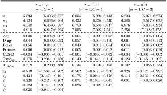
In Table 2, we report parameter estimates for the longitudinal data model, with 95% confidence intervals (in brackets) based onB = 1000bootstrap re-samples. By looking at the estimates of fixed Table 2. CD4 data -lqmHMM: parameter estimates for the longitudinal model at different quantiles.95% bootstrap confidence intervals are reported in brackets.
τ=0.25 τ=0.50 τ=0.75 [m= 4, G= 5] [m= 4, G= 4] [m= 4, G= 3] α1 5.593 (5.403; 5.677) 6.054 (5.994; 6.133) 6.203 (6.071; 6.273) α2 6.124 (6.066; 6.166) 6.432 (6.368; 6.530) 6.580 (6.517; 6.628) α3 6.540 (6.489; 6.587) 6.750 (6.689; 6.837) 6.876 (6.804; 6.934) α4 6.915 (6.847; 6.995) 7.055 (7.023; 7.231) 7.256 (7.168; 7.373) Age 0.000 (−0.004; 0.002) 0.004 (−0.001; 0.008) 0.000 (−0.005; 0.005) Drugs 0.044 (0.000; 0.092) 0.057 (−0.014; 0.110) 0.061 (0.003; 0.113) Packs 0.056 (0.041; 0.071) 0.043 (0.015; 0.054) 0.044 (0.015; 0.062) Partners 0.006 (0.001; 0.012) 0.005 (0.001; 0.012) 0.011 (0.003; 0.016) CES-D −0.004 (−0.005;−0.001) −0.004 (−0.006;−0.002) −0.004 (−0.006;−0.002) Timesero −0.175 (−0.206;−0.150) −0.140 (−0.164;−0.114) −0.123 (−0.145;−0.102) σTimesero 0.219 (0.200; 0.360) 0.134 (0.105; 0.165) 0.102 (0.088; 0.133) ζ1 -0.849 (−1.568;−0.802) -0.502 (−0.617;−0.370) -0.328 (−0.423;−0.297) ζ2 -0.434 -(0.447;−0.401) -0.175 (−0.204;−0.158) -0.114 (−0.130;−0.093) ζ3 -0.220 (−0.245;−0.203) -0.071 (−0.104;−0.061) -0.001 (−0.020; 0.020) ζ4 -0.123 (−0.141;−0.099) 0.026 (−0.027; 0.037) ζ5 -0.020 (−0.041;−0.004)
model parameters, we may notice slight differences with respect to the results discussed for thelqmm. In particular, if we look at significance levels, these generally agree but for Drugs; the estimate at τ= 0.25forlqmmis not included in the confidence interval for the same parameter under thelqmHMM specification. This may be due to some form of aliasing between the categorical covariate and the time-constant locations. Further differences are observed for the marginal estimate of Timesero and the
corresponding standard deviation. In particular, forτ = 0.25, the effect of the time since seroconversion is slightly higher underlqmHMMwith respect tolqmm, while this effect is attenuated forτ = 0.50,0.75. On the other hand, estimates ofσTimesero are globally higher (for all analysed quantiles) when considering thelqmHMMspecification. As regards the estimated random intercepts (αh), we notice that the estimates tend to increase with τ and this is consistent with increasing values of the baseline (log) CD4 levels. Table3reports the estimates for the initial and the transition probabilities of the hidden Markov chain. The combination of these results with the intercept values reported in Table2give some hints on the
dynamics of the response variable. The estimated initial probabilities suggest that most of the individuals Table 3. CD4 data -lqmHMM: initial and transition probability estimates at different quantiles.95%bootstrap confidence intervals are reported in brackets.
1 2 3 4 τ=0.25 δ 0.083 (0.036; 0.134) 0.408 (0.316; 0.512) 0.411 (0.304; 0.501) 0.098 (0.055; 0.157) 1 0.284 (0.116; 0.466) 0.700 (0.510; 0.860) 0.000 (0.000; 0.025) 0.016 (0.000; 0.069) 2 0.083 (0.034; 0.125) 0.675 (0.574; 0.754) 0.232 (0.153; 0.334) 0.010 (0.000; 0.032) 3 0.031 (0.008; 0.062) 0.126 (0.077; 0.179) 0.787 (0.705; 0.844) 0.055 (0.019; 0.119) 4 0.011 (0.000; 0.033) 0.044 (0.000; 0.090) 0.015 (0.000; 0.095) 0.930 (0.854; 0.977) τ=0.50 δ 0.120 (0.059; 0.242) 0.434 (0.306; 0.543) 0.326 (0.213; 0.449) 0.120 (0.059; 0.162) 1 0.927 (0.775; 1.000) 0.073 (0.000; 0.216) 0.000 (0.000; 0.034) 0.000 (0.000; 0.016) 2 0.107 (0.052; 0.174) 0.830 (0.734; 0.925) 0.063 (0.000; 0.144) 0.000 (0.000; 0.016) 3 0.013 (0.000; 0.062) 0.055 (0.000; 0.108) 0.898 (0.838; 0.961) 0.034 (0.000; 0.071) 4 0.043 (0.000; 0.079) 0.000 (0.000; 0.041) 0.019 (0.000; 0.092) 0.938 (0.866; 0.994) τ=0.75 δ 0.119 (0.041; 0.192) 0.359 (0.224; 0.497) 0.367 (0.232; 0.488) 0.155 (0.098; 0.217) 1 0.861 (0.757; 0.958) 0.139 (0.041; 0.243) 0.000 (0.000; 0.000) 0.000 (0.000; 0.000) 2 0.125 (0.069; 0.194) 0.810 (0.701; 0.885) 0.065 (0.000; 0.171) 0.000 (0.000; 0.022) 3 0.021 (0.000; 0.062) 0.094 (0.031; 0.184) 0.858 (0.770; 0.921) 0.026 (0.000; 0.063) 4 0.019 (0.000; 0.048) 0.000 (0.000; 0.044) 0.088 (0.007; 0.192) 0.894 (0.782; 0.965)
in the sample starts the study with intermediate levels of CD4 counts (δ2+δ3>0.70), and only few of
them shows more extreme (lower or higher) levels. Forτ = 0.50,0.75, transitions across hidden states are quite unlikely (qhh>0.8, h= 1, . . . , m) and, if any transition is observed, subjects tend to move towards states with a lower intercept value, with a moderate reduction in the CD4 counts. Forτ= 0.25, we observe a slightly different evolution of the response. Estimated transition probabilities highlight that, for less healthy men, the log-count of CD4 cells in the blood tends to repeatedly increase and decrease over the time, particularly for hidden states with lower intercept values. Transitions towards the first state (with the lowest CD4 log count) are unlikely(Pmk=1qk1<0.15)and, if any transition is observed,
in the next occasion individuals move towards states characterised by higher levels (q11= 0.284). This
indicates that the sudden transition to the fist hidden state is just temporary, with subsequent up and down jumps that render the left tail of the (conditional) response distribution quite unstable. In the last panel of Table2, we report the estimated values of the slope for the covariate Timesero. As it is clear, increasing
values of this covariate correspond to a substantial decrease of the response. This effect progressively reduces when moving across components: individuals belonging to the former classes show a steeper reduction in the (log) CD4 as the time since seroconversion increases. Also, when moving fromτ = 0.25
5.4
Looking at drop-out patterns: the lqHMM+LDO
As previously stated, individuals were observed up to12occasions and only few of them have complete data records. Figure2shows the mean response distribution at each visit stratified by whether subjects drop-out from the study between the current and the next occasion. As it can be seen, CD4 levels for Figure 2. CD4 data - Distribution of the response variable at each time occasion.
6.0 6.2 6.4 6.6 6.8 1 2 3 4 5 6 7 8 9 10 11 12 Time Occasion Mean log(count +1)
Overall Next Measure Available Next Measure Unavailable
individuals dropping-out prematurely are much lower than those observed for individuals that remain under observation. This is particularly evident when the subject is lost at the beginning of the study. Therefore, we may expect that healthier individuals stay longer into the study; the selective participation in the study may question the reliability of the results discussed in the previous sections. For this purpose, we estimated the followinglqHMM+LDO
µit[sit, cig = 1, τ] =x0itβ+z 0 itζg+w 0 itαsit, Pr g X l=1 cil= 1|Ti, τ = exp (λ0g+λ1Ti) 1 + exp (λ0g+λ1Ti) ,
and compared the results with those we obtained from thelqmHMMmodel in Section5.3. The vectors xit,zit andwitare defined as in the last section and parameters have all the same interpretation apart from the random slope for Timesero, which is now assumed to vary with LDO classes. We estimated
the proposed model for τ={0.25,0.50,0.75} and for a varying number of states and LDO classes (m,G=1, . . . ,6). To avoid local maxima, model parameters were initialised via the same multi-start strategy used forlqmHMM. For each[m, G]-combination, we considered30starting points and retained the solution with the lowest BIC value. According to results reported in the Supplementary Material,
we selected the model withm= 5hidden states andG= 5LDO classes forτ= 0.25; for the median and the third quartile the solution withm= 4andG= 4provides the lowest BIC value. Examining the parameter estimates for the LDO class model atτ= 0.75, we noticed that twoλ0gdid not significantly differ from zero and the corresponding confidence intervals substantially overlapped. Therefore, for this quantile, to avoid spurious solutions, we performed the search for the optimal number of classes in the setG≤3. As a result, the best fit corresponds tom= 4hidden states andG= 3LDO classes.
In Table4, we report the parameter estimates for the longitudinal and the missing data models with the corresponding95%confidence intervals (in brackets), based onB= 1000block bootstrap re-samples. Comparing the estimates for the fixed parameters to those we obtained by fitting thelqmHMM(see Table Table 4. CD4 data -lqHMM+LDO: parameter estimates for the longitudinal and the LDO class model at different quantiles.95%bootstrap confidence intervals are reported in brackets.
τ=0.25 τ=0.50 τ=0.75 [m= 5, G= 5] [m= 4, G= 4] [m= 4, G= 3] α1 5.046 (3.937; 5.286) 6.043 (5.931; 6.114) 6.198 (6.069; 6.282) α2 5.880 (5.730; 5.918) 6.416 (6.323; 6.502) 6.579 (6.512; 6.628) α3 6.193 (6.126; 6.256) 6.719 (6.647; 6.825) 6.872 (6.801; 6.934) α4 6.582 (6.508; 6.634) 7.040 (6.973; 7.215) 7.243 (7.167; 7.370) α5 6.936 (6.846; 7.026) Age −0.004 (−0.007; 0.000) 0.004 (−0.001; 0.007) 0.000 (−0.004; 0.005) Drugs 0.048 (−0.013; 0.124) 0.072 (−0.006; 0.145) 0.064 (0.007; 0.115) Packs 0.032 (0.024; 0.051) 0.042 (0.014; 0.054) 0.044 (0.018; 0.064) Partners 0.011 (0.005; 0.016) 0.005 (0.000; 0.012) 0.011 (0.002; 0.016) CES-D −0.003 (−0.006;−0.001) −0.004 (−0.006;−0.002) −0.004 (−0.006;−0.002) Timesero −0.157 (−0.187;−0.127) −0.146 (−0.175;−0.119) −0.131 (−0.155;−0.108) ζ1 -0.740 (−1.079;−0.662) -0.497 (−0.667;−0.452) -0.327 (−0.414;−0.287) ζ2 -0.300 (−0.324;−0.256) -0.176 (−0.200;−0.155) -0.113 (−0.131;−0.093) ζ3 -0.164 (−0.181;−0.133) -0.070 (−0.098;−0.056) 0.003 (−0.023; 0.019) ζ4 -0.053 (−0.095;−0.035) 0.033 (−0.023; 0.047) ζ5 0.026 (−0.011; 0.045) λ01 −2.385 (−3.583;−1.383) −1.062 (−2.112;−0.241) −0.374 (−1.388; 0.615) λ02 −0.082 (−1.159; 0.993) 1.113 (0.013; 2.102) 2.739 (1.295; 4.379) λ03 1.555 (0.514; 2.627) 4.089 (2.002; 5.299) λ04 3.116 (1.926; 4.388) λ1 −0.174 (−0.290;−0.059) −0.193 (−0.318;−0.065) −0.184 (−0.324;−0.066)
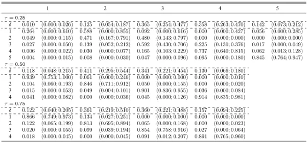
2), we may observe only slight differences. As before, state-dependent intercepts increase when moving from the left to the right tail of the response distribution. By combining these results with the estimated initial and transition probabilities reported in Table5, we draw conclusions that are similar to those for the lqmHMM specification. Only for τ= 0.25we observe a further state with a lower intercept that seems to be linked to the highly variable dynamics for units dropping-out very early. The differences in the Markovian estimates appear to be negligible forτ= 0.50andτ = 0.75.
Table 5. CD4 data -lqHMM+LDO: initial and transition probability estimates at different quantiles.95% bootstrap confidence intervals are reported in brackets.
1 2 3 4 5 τ=0.25 δ 0.010 (0.000; 0.026) 0.125 (0.054; 0.187) 0.365 (0.254; 0.477) 0.358 (0.263; 0.470) 0.142 (0.073; 0.212) 1 0.264 (0.000; 0.610) 0.588 (0.000; 0.855) 0.092 (0.000; 0.616) 0.000 (0.000; 0.427) 0.056 (0.000; 0.285) 2 0.049 (0.000; 0.115) 0.471 (0.167; 0.791) 0.480 (0.143; 0.797) 0.000 (0.000; 0.000) 0.000 (0.000; 0.000) 3 0.027 (0.000; 0.050) 0.139 (0.052; 0.212) 0.592 (0.430; 0.706) 0.225 (0.130; 0.376) 0.017 (0.000; 0.049) 4 0.006 (0.000; 0.022) 0.030 (0.000; 0.077) 0.165 (0.103; 0.229) 0.737 (0.640; 0.815) 0.062 (0.013; 0.128) 5 0.004 (0.000; 0.015) 0.008 (0.000; 0.030) 0.047 (0.000; 0.096) 0.095 (0.000; 0.180) 0.845 (0.764; 0.947) τ=0.50 δ 0.118 (0.048; 0.215) 0.411 (0.295; 0.544) 0.341 (0.221; 0.454) 0.130 (0.066; 0.180) 1 0.939 (0.753; 1.000) 0.061 (0.000; 0.246) 0.000 (0.000; 0.000) 0.000 (0.000; 0.010) 2 0.104 (0.060; 0.193) 0.846 (0.711; 0.912) 0.050 (0.000; 0.155) 0.000 (0.000; 0.020) 3 0.015 (0.000; 0.053) 0.049 (0.004; 0.101) 0.901 (0.836; 0.955) 0.036 (0.000; 0.084) 4 0.041 (0.000; 0.082) 0.000 (0.000; 0.036) 0.045 (0.000; 0.126) 0.914 (0.835; 0.981) τ=0.75 δ 0.122 (0.040; 0.205) 0.361 (0.219; 0.510) 0.360 (0.221; 0.488) 0.157 (0.094; 0.225) 1 0.866 (0.749; 0.973) 0.134 (0.027; 0.251) 0.000 (0.000; 0.000) 0.000 (0.000; 0.000) 2 0.122 (0.065; 0.199) 0.813 (0.695; 0.894) 0.065 (0.000; 0.168) 0.000 (0.000; 0.023) 3 0.020 (0.000; 0.055) 0.099 (0.039; 0.194) 0.854 (0.758; 0.916) 0.027 (0.000; 0.064) 4 0.018 (0.000; 0.045) 0.000 (0.000; 0.045) 0.091 (0.012; 0.207) 0.891 (0.765; 0.960)
LDO-dependent parameters (third panel in Table4) do not substantially differ from those described for thelqmHMMspecification. Units belonging to the first LDO classes experience a steeper decline in the (log) CD4 count as the time since seroconversion increases. This effect is more evident in the left tail of the distribution, while it progressively reduces when moving from the first to the last latent category. The results from thelqHMM+LDOcan be further explored by looking at theλestimates reported in the last panel of Table4. For all quantiles, the negative and significant effect of the time to drop-out (λ1<0)
suggests that the probability of belonging to one of the firstg classes reduces with increasing number of available measures. That is, units in the latter classes present longer longitudinal sequences. Based on this finding, we will refer to “lower” and “higher” LDO classes in what follows.
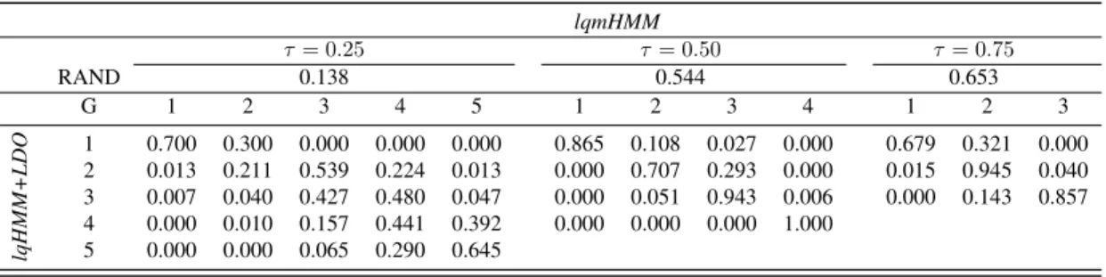
Table6compares the classifications obtained under thelqHMM+LDOand thelqmHMM. In particular, it shows the adjusted RAND index51 forτ ={0.25,0.50,0.75}and the row percentage of individuals classified within different components under the two model specifications.
By looking at the table, it is clear that, generally, the two models lead to similar classifications for τ= 0.50andτ = 0.75, which may suggest a reduced impact of the missing data process on the longitudinal responses for individuals in better health conditions. On the other hand, for the first quartile, that is for less healthy individuals, the classification supplied by the two models appears to be quite different, with an adjusted RAND index equal to0.138. In particular, when adopting thelqHMM+LDO in place of thelqmHMMformulation, we may notice that individuals tend to be shifted towards “lower”
Table 6. CD4 data - Row percentages of individuals classified across components underlqmHMMand lqHMM+LDOat different quantiles.
lqmHMM τ = 0.25 τ = 0.50 τ= 0.75 RAND 0.138 0.544 0.653 G 1 2 3 4 5 1 2 3 4 1 2 3 lqHMM+LDO 1 0.700 0.300 0.000 0.000 0.000 0.865 0.108 0.027 0.000 0.679 0.321 0.000 2 0.013 0.211 0.539 0.224 0.013 0.000 0.707 0.293 0.000 0.015 0.945 0.040 3 0.007 0.040 0.427 0.480 0.047 0.000 0.051 0.943 0.006 0.000 0.143 0.857 4 0.000 0.010 0.157 0.441 0.392 0.000 0.000 0.000 1.000 5 0.000 0.000 0.065 0.290 0.645
components. As discussed before, these are characterised by shorter longitudinal sequences and by a stronger impact (especially in the last occasions) of Timeseroon the CD4 count levels.
5.5
Sensitivity analysis
The results reported in the previous sections, together with the lower BIC values forlqHMM+LDOwhen compared to those observed for lqmmandlqmHMM (see Tables 1-3 in the Supplementary Material), suggest a better fit of the former model to the observed data. Under this model specification, the strength of dependence between the longitudinal process and the missing data mechanism, is assessed via the non-ignorability parameterλ1and the corresponding confidence interval. As highlighted before, results
reported in Table 4 highlights quite a strong association between the two processes. However, when dealing with missingness, we should consider that the observed data contain only limited information on the missing data mechanism, and sensitivity analysis represents a crucial matter. In this perspective, the comparison between the fixed parameter estimates in the longitudinal data model obtained under the lqmHMM(Table2) and thelqHMM+LDOformulation (Table4), is of major interest. As we may notice by looking at the tables, estimates are quite similar, thus suggesting a certain degree of robustness of the proposed models with respect to possible misspecification of the missing data mechanism.
Also, a key assumption of thelqHMM+LDOis the conditional independence between the longitudinal and the missing data process, given the LDO class membership. This assumption may be questionable and may be appropriate for the observed data only. We may follow an approach similar to Roy and Daniels22 and Dantan et. al.40 to formally test this hypothesis, at least for the observed data. For each quantile and for the chosen[G, m]combination, we estimated alqHMM+LDOadding in the linear predictor the time to drop-out (we will refer to this model specification asMTi(τ)) and its logarithm (we will refer to this model specification asMlogTi(τ)), while keeping fixed the ML estimates for the LDO classes, as well as the corresponding posterior probabilities. It is worth noticing that the logarithmic transform was
considered to make more evident potentially non linear effects of the drop-out time on the longitudinal response. The likelihood values we obtained usingMTi(τ)andMlogTi(τ)were compared to those of the estimatedlqHMM+LDOvia a likelihood ratio test (LRT). Under the hypothesis of a null effect for Ti after controlling for the LDO membership, the LRT would follow an approximate χ2 distribution with ν = 1 degrees of freedom. The p-values obtained for MTi(0.25), MTi(0.50) and MTi(0.75) are{0.24,0.02,0.00}, respectively, while forMlogTi(τ)we obtained{0.72,0.45,0.71}. These results highlight the presence of a residual dependence between the missingness and the longitudinal process for τ= 0.50andτ= 0.75when fittingMTi(τ). However, the only substantial change with respect to the chosen model was found for the Markov-dependent intercepts. To further investigate the conditional independence assumption, we computed the confidence intervals based on B= 1000 bootstrap re-samples for the parameters in MTi(τ). Results are reported in Table7. As it is clear, no substantial Table 7. CD4 data - Conditional independence: Bootstrap confidence intervals for fixed parameters in the longitudinal model at different quantiles.
τ= 0.25 τ = 0.25 τ = 0.25 2.5% 97.5% 2.5% 97.5% 2.5% 97.5% Age -0.006 0.000 0.001 0.006 -0.003 0.004 Drugs 0.001 0.117 -0.016 0.150 0.017 0.099 Packs 0.022 0.047 0.015 0.054 0.021 0.062 Partners 0.006 0.017 0.002 0.013 0.004 0.018 CES-D -0.006 -0.001 -0.006 -0.003 -0.006 -0.002 Ti -0.015 0.005 -0.018 0.002 -0.022 0.003
changes in the significance of the parameters of interest are present and, above all, when conditioning on the LDO class membership, the effect of the time to drop-out on the log CD4 count seems negligible for all the analysed quantiles. Thus, the local independence assumption seems to be quite appropriate.
6
Concluding remarks
We discuss a class of mixed hidden Markov quantile regression models for longitudinal continuous responses. A general dependence structure is considered by allowing the measurements from each individual to share time-varying and time constant random coefficients, extending thelqmm2–4 and the lqHMM14 specifications. Both sources of unobserved heterogeneity are modelled via non-parametric distributions which offer a robust alternative to (possibly unverifiable) parametric assumptions.
The model is further extended to handle non-ignorable drop-out via a pattern mixture representation. We assume that the time-constant random coefficients depend on the observed number of measurements for each individual through an ordered latent class approach. The re-analysis of a well known benchmark
dataset, the CD4 cell count data17;18, reveals the potential impact of drop-out on the lower quantiles of the response variable (conditional) distribution.
7
Supplementary Material
The Supplementary Material includes the computational details for the posterior expectation of the complete data log-likelihood. Also, the results from a large scale simulation study and the tables describing model selection for the CD4 data are reported.
References
1. Lee Y and Nelder J. Conditional and marginal models: Another view.Statistical Science2004; 19: 219–238. 2. Geraci M and Bottai M. Quantile regression for longitudinal data using the asymmetric Laplace distribution.
Biostatistics2007; 8: 140–54.
3. Liu Y and Bottai M. Mixed-Effects Models for Conditional Quantiles with Longitudinal Data.The International Journal of Biostatistics2009; 5: 1–24.
4. Geraci M and Bottai M. Linear quantile mixed models.Statistics and Computing2014; 24: 461–479.
5. Tzavidis N, Salvati N, Schmid T et al. Longitudinal analysis of the strengths and difficulties questionnaire scores of the millennium cohort study children in england using m-quantile random-effects regression. Journal of the Royal Statistical Society: Series A (Statistics in Society)2016; 179: 427–452.
6. Reich BJ, Bondell HD and Wang HJ. Flexible Bayesian quantile regression for independent and clustered data.
Biostatistics2010; 11: 337–352.
7. Yuan Y and Yin G. Bayesian quantile regression for longitudinal studies with nonignorable missing data.
Biometrics2010; 66: 105–114.
8. Koenker R. Quantile regression for longitudinal data.Journal of Multivariate Analysis2004; 91: 74–89. 9. Harding M and Lamarche C. A quantile regression approach for estimating panel data models using instrumental
variables.Economics Letters2009; 104: 133 – 135.
10. Galvao AF and Montes-Rojas GV. Penalized quantile regression for dynamic panel data.Journal of Statistical Planning and Inference2010; 140: 3476–3497.
11. Galvao AF. Quantile regression for dynamic panel data with fixed effects. Journal of Econometrics2011; 164: 142–157.
12. Liu M, Daniels MJ and Perri MG. Quantile regression in the presence of monotone missingness with sensitivity analysis.Biostatistics2016; 17: 108–121.
13. Bartolucci F and Farcomeni A. A multivariate extension of the dynamic logit model for longitudinal data based on a latent markov heterogeneity structure.Journal of the American Statistical Association2009; 104: 816–831.
14. Farcomeni A. Quantile regression for longitudinal data based on latent Markov subject-specific parameters.
Statistics and Computing2012; 22: 141–152.
15. Bartolucci F, Farcomeni A and Pennoni F.Latent Markov Models for Longitudinal Data. Chapman & Hall/CRC Press, 2013.
16. Marino MF and Farcomeni A. Linear quantile regression models for longitudinal experiments: an overview.
METRON2015; 73: 229–247.
17. Kaslow RA, Ostrow D, Detels R et al. The multicenter aids cohort study: rationale, organization, and selected characteristics of the participants.American Journal of Epidemiology1987; 126: 310–318.
18. Zeger SL and Diggle PJ. Semiparametric models for longitudinal data with application to CD4 cell numbers in HIV seroconverters.Biometrics1994; 50: 689–699.
19. Farcomeni A and Viviani S. Longitudinal quantile regression in presence of informative drop-out through longitudinal-survival joint modeling.Statistics in Medicine2015; 34: 1199–1213.
20. Marino MF and Alf´o M. Latent drop-out based transitions in linear quantile hidden markov models for longitudinal responses with attrition.Advances in Data Analysis and Classification2015; 9: 483–502. 21. Roy J. Modeling longitudinal data with nonignorable dropouts using a latent dropout class model. Biometrics
2003; 59: 829–836.
22. Roy J and Daniels M. A general class of pattern mixture models for nonignorable dropout with many possible dropout times.Biometrics2008; 64: 538–545.
23. Daniels MJ and Hogan JW. Missing Data in Longitudinal Studies: Strategies for Bayesian Modeling and Sensitivity Analysis. Chapman & Hall / CRC Press, 2008.
24. Yu K and Zhang J. A three-parameter asymmetric Laplace distribution and its extension. Communications in Statistics - Theory and Methods2005; 34: 1867–1879.
25. Koenker R and Bassett G. Regression quantiles.Econometrica1978; 46: 33–50.
26. Marino MF and Alf´o M. Gaussian quadrature approximations in mixed hidden markov models for longitudinal data: A simulation study. Computational Statistics & Data Analysis2016; 94: 193 – 209.
27. Laird N. Nonparametric maximum likelihood estimation of a mixing distribution. Journal of the American Statistical Association1978; 73: 805–811.
28. Dempster A, Laird NM and Rubin DB. Maximum likelihood from incomplete data via the EM algorithm.
Journal of the Royal Statistical Society Series B (Methodological)1977; 39: 1–38.
29. Aitkin M. A general maximum likelihood analysis of variance components in generalized linear models.
Biometrics1999; 55: 117–128.
30. Demirtas H and Schafer JL. On the performance of random-coefficient pattern-mixture models for non-ignorable drop-out.Statistics in medicine2003; 22: 2553–2575.
32. Heckman JJ. The common structure of statistical models of truncation, sample selection and limited dependent variables and a simple estimator for such models. InAnnals of Economic and Social Measurement. 1976. pp. 475–492.
33. Little RJA. Pattern-mixture models for multivariate incomplete data. Journal of the American Statistical Association1993; 88: 125–134.
34. Wu MC and Carroll RJ. Estimation and comparison of changes in the presence of informative right censoring by modeling the censoring process.Biometrics1988; : 175–188.
35. Wulfsohn MS and Tsiatis AA. A joint model for survival and longitudinal data measured with error.Biometrics
1997; : 330–339.
36. Little RJA. Modeling the drop-out mechanism in repeated-measures studies.Journal of the American Statistical Association1995; 90: 1112–1121.
37. Rizopoulos D and Lesaffre E. Introduction to the special issue on joint modelling techniques.Statistical Methods in Medical Research2014; 23: 3–10.
38. Bartolucci F and Farcomeni A. A discrete time event-history approach to informative drop-out in mixed latent markov models with covariates.Biometrics2015; 71: 80–89.
39. Maruotti A. Handling non-ignorable dropouts in longitudinal data: a conditional model based on a latent markov heterogeneity structure.TEST2015; 24: 84–109.
40. Dantan E, Proust-Lima C, Letenneur L et al. Pattern mixture models and latent class models for the analysis of multivariate longitudinal data with informative dropouts.International Journal of Biostatistics2008; 4: 1–26. 41. Ma G, Troxel AB and Heitjan DF. An index of local sensitivity to nonignorable drop-out in longitudinal
modelling.Statistics in Medicine2005; 24: 2129–2150.
42. Agresti A.Analysis of Ordinal Categorical Data. John Wiley & Sons, 2010.
43. Baum LE, Petrie T, Soules G et al. A maximization technique occurring in the statistical analysis of probabilistic functions of Markov chains.The Annals of Mathematical Statistics1970; 41: 164–171.
44. Welch LR. Hidden Markov models and the Baum-Welch algorithm. IEEE Information Theory Society Newsletter2003; 53: 10–13.
45. Akaike H. Information theory and an extension of the maximum likelihood principle. In Petrov BN and Csaki F (eds.)Second International Symposium on Information Theory. Akad´emiai Kiado, pp. 267–281.
46. Schwarz G. Estimating the dimension of a model.The Annals of Statistics1978; 6: 461–464.
47. Jones RH. Bayesian information criterion for longitudinal and clustered data. Statistics in Medicine2011; 30: 3050–3056.
48. Lahiri S. Theoretical comparisons of block bootstrap methods.Annals of Statistics1999; 27: 386–404. 49. Buchinsky M. Estimating the asymptotic covariance matrix for quantile regression models. A Monte Carlo
50. Radloff LS. The CES-D scale a self-report depression scale for research in the general population. Applied Psychological Measurement1977; 1: 385–401.
51. Rand WM. Objective criteria for the evaluation of clustering methods. Journal of the American Statistical Association1971; 66: 846–850.