Methods and Tools for Visual Analytics.

(1)

Methods and Tools for Visual Analytics

by Hao Zhou

A dissertation submitted in partial fulﬁllment of the requirements for the degree of

Doctor of Statistics (Statistics)

in The University of Michigan 2011

Doctoral Committee:

Professor George Michailidis, Chair Professor Hosagrahar V. Jagadish Associate Professor Kerby A Shedden Associate Professor Ji Zhu

(2)

c

(3)

(4)

ACKNOWLEDGEMENTS

First and foremost, I would like to thank my advisor, Professor George Michailidis. He has unstintingly shared his fantastic excitement about, and knowledge of, statis-tical methods and visual analytics. He has introduced me to these beautiful subjects. In addition, he has kept me motivated throughout my graduate school years.

I have received generous support from Professor Hosagrahar V. Jagadish, who also guided me to work on the visual analytic algebra project. Discussions with him and his student, Anna A. Shaverdian, have substantially deepened my understanding of the system design. All of these are crucial in shaping my thesis.

(5)

LIST OF FIGURES

Figure

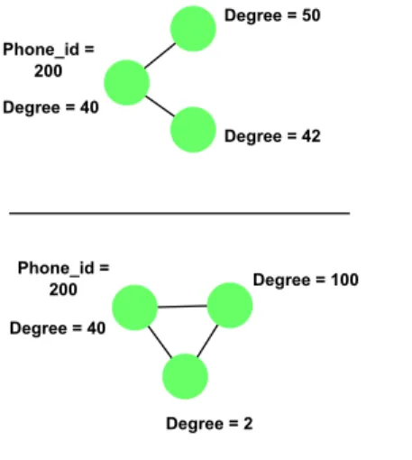
2.1 The ﬁgure shows a simple predicate corresponding to the cross-referencing example. Conditions are placed upon the attributes on the nodes. It is possible for one condition to reference the attribute on another node. 13 2.2 These graph structures satisfy the predicate shown in Figure 2.1.

They are two possible instantiations of the predicate. . . 13 2.3 The two predicates show similar graph structures. However, the

fig-ure on the left has an excluded edge between nodes 2 and 3. Figfig-ure 2.4 shows the result of this excluded edge on possible witnesses given an input graph. . . 14 2.4 The figure above is an input graph. Given the two predicates shown

in Figure 2.3 we describe the diﬀerent witnesses existing in this input graph. The sets of nodes which induce a witness to the excluded edge predicate are: 1,2,3 and 2,4,3. The predicate without the excluded edge results has more witnesses: 1,2,3; 1,2,4; 1,4,3; 2,4,3; and more. Since there is an edge between node 1 and 4, this the witness 1,2,4 does not satisfy the predicate with the excluded edge. . . 14

2.5 The Graph Matching function takes two inputs: a graph and a pred-icate. Given these inputs, the graph matching function will ﬁnd wit-nesses that satisfy the predicate within the input graph. . . 17

(9)

2.6 Given the inputs to the graph matching function shown in Figure 2.5, the function will return three types of output. First there exists one witness in the input graph. Second, a model witness is returned that maintains the predicate structure. In this case, the model witness is identical to the witness. But it is possible the witness contains an edge between nodes 1 and 3 and still be a witness to the predicate. The last structure returned is a mapping list for the witness to the model witness. The mapping list is useful for the analyst to see how the witness matches the predicate. The mapping list in this case is: {1→6,2→7,3→8,4→9} . . . 17 2.7 Two input attributed graphs are displayed. If the predicate to the

set selection function is that the graph attribute, average degree, be equal to 2, then the result from set selection is the input graph shown on the left. The input graph shown on the right has an average degree of 1.67. . . 19 2.8 Given the two input graphs and the predicate shown above, the

re-sulting attributed graph after an element selection call is shown. The input graph contains a witness for the predicate, namely the witness induced by the node set (16,17,18,19). The input graph on the right has no witness for the given predicate. The graph matching function is called to determine if a witness exists in an input graph. . . 19

2.9 An element aggregation by all structures is performed on the input graph. The result is the blue nodes are merged into one group, and the purple nodes into a second group. . . 23 2.10 After an element aggregation by structure, the attributed graph

be-comes only three nodes. . . 24 2.11 The three aggregated nodes in the merged graph of Figure 2.10 point

to a model witness. The purpose of this model witness is the retain the predicate structure, the reason for the aggregation, to understand the analytical process. . . 24

2.12 A labeling function performed on the same input graph and predicate from the element selection example, Figure 2.8 . . . 26

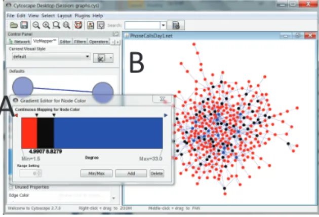
2.13 A continuous color gradient mapping to node degree is set on the phone data set from the VAST 2008 Challenge. . . 29

(10)

2.14 As part of our Visual Analytic Algebra, we deﬁne attributes as either computed or intrinsic. To allow the user to modify the type of an attribute we provide the following tab under the Control Panel. The user can view the attribute labels for nodes, edges, and the graph. To change the type from intrinsic to computed, the user can drag the attribute label from one type to another. . . 30 2.15 The main Cytoscape window is shown. There are three main

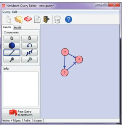
com-ponents to its design. The network panel displays the network. The data panel displays node and edge specific attribute information. The control panel has several tabs to perform different functions on the network. One of these tabs is the network tab, that shows all the net-works opened during a current Cytoscape analysis session. It allows the user to switch between different networks by saving them under different names. . . 31 2.16 The plugin NetMatch allows a user to draw a query. In essence, a

query is a predicate. Attribute conditions are possible on nodes. . . 31 2.17 Using the NetMatch plugin, we show the result of matching the input

graph and the predicate shown in Figure 2.5. The image shown is a witness found in the input graph. The Node column shows the map-ping between the witness and the predicate. This ﬁgure is an example implementation of the Predicate, Witness, and Graph Matching fea-tures in the Visual Analytic Algebra. . . 32 2.18 The Visual Analytic Graph Algebra Plugin also includes an

Opera-tors Tab in the Control Panel. Here the analyst can select a set of networks, the predicate list, and the operator to apply to the graphs. In this ﬁgure, the set selection Operator has been selected with the Predicate from Figure 2.1. . . 33 2.19 This ﬁgure shows an example implementation of set selection in

Cy-toscape. Once the ”Done” button has been clicked, the result of the set selection is the set of graphs that satisfy the predicate are opened and displayed in the Display Panel. In this ﬁgure, four graphs are displayed. . . 33 2.20 This ﬁgure shows (1) the input graph, (2) the predicate, and (3) the

results from element selection. . . 34 2.21 On the Operators Tab, the drop down menu shown has all of the

(11)

2.22 A Cytoscape Aggregation by All Structures is performed on the input graph shown on the left. . . 35 2.23 A Cytoscape Aggregation Per Structures is performed on the input

graph shown on the left. . . 35 2.24 The graph on the left is what the ﬁnal graph after the analysis should

be. The graph on the right shows one of the graphs produced during the user study. . . 37 2.25 Starting from the graph on the left, the graph on the right is created,

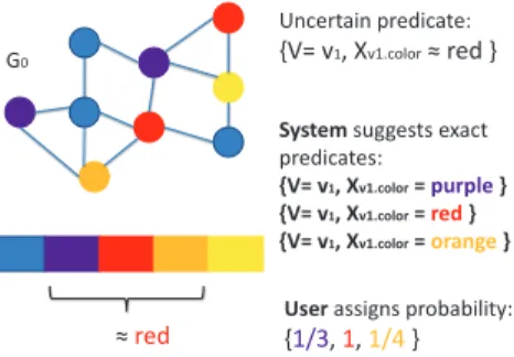
the summarized graph. . . 38 3.1 Example to transform a categorical uncertain predicate into a set of

exact predicates. . . 44 3.2 Example of edge certainty. Dash line stands for uncertain connections 44

3.3 Example of element selection based on an uncertain predicate α∗ in blue. The numbers inside the node denote the id. The numbers outside the node denote the age attribute’s value. The diﬀerent col-ors are used for visualization clarity. The pink represents input and output graphs. The blue represents predicates. And the light green represents witnesses. . . 49 3.4 Example of element aggregation. . . 51

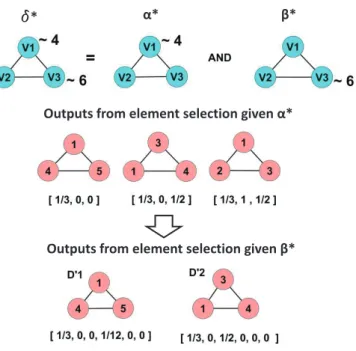
3.5 Example of joint element selection. The selection operator with un-certain predicate α∗ AND β∗ is split into two. One split selection has uncertain predicateα∗ and the other has uncertain predicateβ∗ 53 3.6 This ﬁgure shows that we get the same outputs as the combined

uncertain predicate structure if we split the predicate structure into

(12)

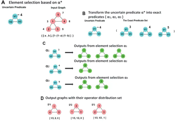
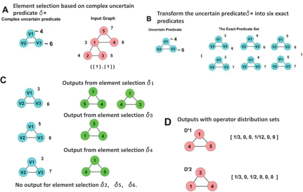
3.7 This example shows a complicated uncertain predicate structure with two attribute value uncertainties. Part A shows the uncertain predi-cate and the attributed graph D. Part B shows the uncertain pred-icate transform into a set of six exact predpred-icates. Part C shows the output from exact element selection. Finally, Part D shows the ﬁ-nal output with its operator distribution set. The numbers inside the node denote the id. The numbers outside the node denote the age attribute’s value. The diﬀerent colors are used for visualization clarity. The pink represents input and outputs graphs. The blue represents predicates. And the light green represents outputs from exact matching problems. . . 55

3.8 Example of a workﬂow of an analysis with usage of visualization function. . . 58

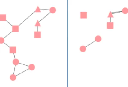
3.9 This ﬁgure shows that the suspect criminal network structure for the Flitter study. Dashlines stand for uncertain connections. . . 59

3.10 Overview of the Flitter network. . . 60 3.11 Workﬂow of Flitter study analytic process. . . 60 3.12 Two output graphs from the ﬁrst selection component. Number in

each node is the user ID. The output probability for the upper graph is 1₂ and the output probability for the lower graph is 1₃, because of the degree diﬀerences between two middleman, user 4994 and 4980. 63

4.1 A two-dimensional visual representation of penalty functions. . . 71 4.2 Network constraint of the synthetic data set. Color of the node

rep-resents its membership to a connected subgraph. . . 73 4.3 Principal component analysis output for the synthetic data set (Top

Left). Linear discriminant analysis output for the synthetic data set(Top Right) with overlapping nodes are 9 and 16. NPSVD outputs with diﬀerent network constraints (Bottom). . . 74 4.4 Movie network contains 558 movies (nodes) from the year of 1916

to 2005. The color of nodes represents as type of each movie. Two movies are connected, if they share at least one common category. . 76 4.5 Two dimensional PCA projection of movie ratings . . . 77 4.6 Two dimensional network PSVD display of movie ratings . . . 78

(13)

4.7 Two dimensional PCA projection of a set of movie ratings . . . 78

4.8 Two dimensional PCA and network PSVD projections of a set of movie ratings . . . 79

4.9 Scatterplot matrix for all seven variable in the star dataset. Black nodes correspond to actors and red nodes correspond to actress in the dataset. The seven variables are average number of votes, reviews and critics, average ratings, average revenue from the ﬁrst opening weekend, average box-oﬃce gross and the total number of movie one made between 1990 to 1995. . . 81

4.10 Network for all 18 stars. The wider the edge width implies more frequent collaborations. . . 82

4.11 PCA output is constructed based only on the seven input variables, while Network penalized SVD output is constructed based on both characteristic and structural information . . . 83 4.12 Biological network contains two gene pathways. . . 86

4.13 Two dimensional PCA projection of gene expression levels. . . 86 4.14 Two dimensional NPSVD projection of gene pathway dataset. . . . 87 5.1 Box plot of testing errors over 200 cross validations. Red, green and

blue box plots are constructed based on testing errors from multi-task, individual training and pooled methods. From the left column to the right column, signal to noise ratio decreases. . . 101

5.2 Bootstrapping results from both multi-task and individual methods for some of estimated parameters. . . 102

5.3 Box plot of testing errors over 200 cross validations under diﬀerent generalized signal to noise ratios. Red, green and blue box plots are constructed based on testing errors from multi-task, individual training and pooled methods. The estimated generalized signal to noise ratios range from 5 to 50. . . 103

5.4 Box plot of testing errors over 200 cross validations from weight with white noise simulation. Red, green and blue box plots are con-structed based on testing errors from multi-task, individual training and pooled methods. . . 105 5.5 Box plot of testing errors from 514 users over 50 cross validations. . 107

(14)

5.6 Closer look at testing errors from 514 users for multi-task and indi-vidual learning methods. . . 108 5.7 The edge weight distribution of movie preference network. . . 108 5.8 Movie Preference Network, where nodes are users and edges are

sim-ilar movie preferences.From the top network to the bottom network, we select edges with high similarity level. Node color stands for dif-ferent age groups (below age 25 = yellow, 25- 35 age group = orange , above 45 group = red). . . 110

(15)

ABSTRACT

Methods and Tools for Visual Analytics by

Hao Zhou

Chair: George Michailidis

Technological advances have led to a proliferation of data characterized by a complex structure; namely, high-dimensional attribute information complemented by relation-ships between the objects or even the attributes.

Classical data mining techniques usually explore the attribute space, while net-work analytic techniques focus on the relationships, usually expressed in the form of a graph. However, visualization techniques oﬀer the possibility to gain useful in-sight through appropriate graphical displays coupled with data mining and network analytic techniques.

In this thesis, we study various topics of the visual analytic process. Speciﬁcally, in chapter 2, we propose a visual analytic algebra geared towards attributed graphs. The algebra deﬁnes a universal language for graph data manipulations during the visual analytic process and allows documentation and reproducibility. In chapter 3, we extend the algebra framework to address the uncertain querying problem. The algebra’s operators are illustrated on a number of synthetic and real data sets, im-plemented in an existing visualization system (Cytoscape) and validated through a small user study.

(16)

In chapter 4, we introduce a dimension reduction technique that through a reg-ularization framework incorporates network information either on the objects or the attributes. The technique is illustrated on a number of real world applications.

Finally, in the last part of the thesis, we present a multi-task generalized linear model that improves the learning of a single task (problem) by utilizing information from connected/similar tasks through a shared representation. We present an algo-rithm for estimating the parameters of the problem eﬃciently and illustrate it on a movie ratings data set.

(17)

CHAPTER I

Introduction

As technology advances daily, demands for processing complex high dimensional graphical data become increasingly needed in various ﬁelds. For example, in the study of social computing network, network structure contains communication information among user, while user logs provide addition characteristic information on the indi-vidual level. Moreover, in many biology studies, researchers collect expression levels for genes. The tested genes are often functionally related, while patients may be blood-related in the study of inherited diseases.

In recent years, many studies have shown that a mixture of human and machine intelligence can often be much more eﬀective than either on alone. Since visualization is the most intuitive and direct way of learning for data, visual analytic, which is the science of analytic reasoning through visual interaction, has received a lot of attention as evidenced by large number of tools and algorithms developed for this purpose.

In order to use these tools and algorithms, one often needs to go through a growing body of literature on visual analytic systems. In addition, it is difficult to find precise documentation for how a visualization was created to display results of a given study; therefore, it creates limitation on replicating others’ work. Furthermore, many visual analytic tools are centered on a particular type of application, such as biological data, then there is no clear translation technique to replicate the tool’s benefits and function

(18)

for other applications. The underlying cause for all these problems is the lack of a systematic method to design graph tools. There is no universal language that deﬁnes the basic graph data manipulation actions in visual analytics.

In the second chapter of the thesis, we present a visual analytic graph algebraic method to solve those problems. The visual analytic graph algebra is part of a frame-work with the following components:(1) a formalized graph model, (2) an expressive predicate language, and (3) an algebra with associated operators and functions. The purpose of the operators is to manipulate the raw graph data during a visual analytic process. The selection operator zooms into a region of interest. The aggregation op-erator manipulates the data resolution with super nodes.The labeling function tracks notable information collected during an analysis, which is useful during lengthy anal-ysis. And finally, the Visual function incorporates the interactive aspect of visual analytics in a work flow, which makes a visualization creation stage as flexible as the data manipulation stage. The benefits of an algebra are now we can systematically replicate,compare, and assess graph visual analytics. Thus, a visual analytic algebra facilitates the production of graph information analysis. To show the practical us-age of the algebra, we incorporate it into an existing graph analysis tool, Cytoscape. Moreover, we demonstrate the uncertainty model on a synthetical data analysis. Fi-nally, we conduct a user study to examine its effectiveness in visual analytic work reproducibility.

In the third chapter, we propose an uncertain model based on the existing algebraic framework to handle uncertainty in the querying workﬂow. It is constructed from a user deﬁned probability set based on the given uncertain query, where the probability describes how well the given outputs capture the user’s target structure. Instead of only dealing a single uncertain query analytic step, it provides the user a systematic way of ranking all outputs for a multi-step visual analytic process.

(19)

process, one should always visualize the data to have a basic understanding of the given information. There are many existing visualization methods, for example, Scat-ter plot, Principle Component Analysis and many classiﬁcation methods. ScatScat-ter plot provides only 2-dimensional view of data at a time. It is often time consuming and misleading, when one tries to work with high dimensional data. Principle component analysis projects high dimensional data information into a low dimensional space by maximizing sample variance. It often give a quick summarization of the high dimen-sional information, however, it cannot capture any relationship among all observations by PCA’s independent assumption. If the relationship among all observation can be fully captured by a group label, many existing classiﬁcation method can be used for the visualization purpose. For example, linear discriminate analysis projects the high dimensional data information into a low dimensional space while preserving between group separations. When the relationships within the dataset become even more com-plicated, which cannot be explained by a single grouping label, existing dimension reduction methods fail to capture the entire complex data information. Some existing visual analytic systems tries to solve this problem by introducing a user interactive feature where one can visualize and work with multiple graphs at once; however, such attempt is also problematic due to the physical limitation of the screen space.

In the fourth chapter of the thesis, we introduce a dimension reduction method based on regular Singular Value Decomposition to address the problem of visualizing complex high dimensional data structures containing information among observations and multiple characteristics. Our approach is to incorporate network information by using penalty functions. We put connected observations together and let them have similar coordinates in the constructed low dimensional space. We demonstrate the performance of the network penalized singular value decomposition method on both synthetic data set and real world applications.

(20)

relationship within the given information, but also predicate behaviors for the future application. Existing machine learning methods are often used to solve the predi-cation problem. Besides of observing a single high dimensional variable to describe characteristic information for each node/object in the network, we obtain multiple observations for each object, such as repeating measurements of the same object. In usual machine learning setup, we treat all information on each node as an independent task and build a leaner to understand the behavior for the single task. However, since in our case, we have the information of relationship among all nodes, the additional structure has been successfully used to improve the prediction model.

In the last chapter of the thesis, we introduce a multi-task machine learning method based on existing generalized linear model. Instead of treating each node or subject as a single independent learning task that was done by our predeces-sors, our contribution is constructing a learning model for each task based on all related/connected tasks. We demonstrate the performance of our model by compar-ing the predication error rate between the generalized linear multi-task model to other existing approaches on both synthetic dataset and real world applications. Last, we adopt bootstrapping method for the statistical inference.

(21)

CHAPTER II

Visual Analytic Algebra

2.1 Introduction

Visual Analytics is the science of analytical reasoning through visual interaction. In recent years there has been growing interest in this field as people recognize that a mix of human and machine intelligence can often be much more effective than either one alone. Graphs are ubiquitous in many scientific fields: high-throughput “omic” sciences use graphs to study pathways, computer networks use graphs to analyze communications, and almost everyone is involved in the explosive growth of online social networks. Graphs are also particularly amenable to visual representation.

It is no surprise that graph visual analytics has received a lot of attention as evidenced by the large number of tools and algorithms developed for this purpose. (See Related Work Section below). Using these tools and algorithms, there is also a growing body of literature describing both visual analytics systems, as well as problems successfully addressed through visual analytics. These systems can be very informative, but usually constrain the reader in realizing their full value for several reasons, listed below.

One problem is assessing the completeness of a tool’s exploration abilities. Science has not put a bound on an analyst’s ability to explore graph data and produce ﬁndings. But, if the basic functions to manipulate and represent data during the

(22)

analysis is enumerated, then assessing which tool is ”better” in an exploration task is possible because then the functions each tool oﬀers can be compared.

Another problem is replication, an important tenet of science. For example, if one tool is created for a biological application, there is no universal systematic way to replicate it for other types of applications.

The underlying cause for these problems is the lack of a systematic method to design graph tools. There is no common language that deﬁnes the basic graph data manipulation actions in visual analytics. Towards this goal, we present a visual analytic graph algebra to meet this void. The visual analytic graph algebra is part of a framework with the following components: (1) a formalized graph model, (2) graph data manipulation operations, and (3) an expressive predicate language.

The purpose of the operators is to manipulate the raw graph data before applying a visualization scheme. The selection operator zooms into a region of interest. The aggregation operator manipulates the data resolution with supernodes. The labeling function tracks information, which is useful during lengthy analysis. And finally, the visual function incorporates the interactive aspect of visual analytics in a work flow, which makes visualization as flexible as the data manipulation stage.

The beneﬁts of an algebra are that one can systematically replicate, compare, and assess diﬀerent graph visual analytics. Thus, a visual analytic algebra facilitates the production of graph information analysis. Based on the existing algebra, we also introduce an uncertainty model to handle queries. We propose a systematical ranking of outputs for an analytic process.

Further to make the algebra suitable for application, we present an implementation in Cytoscape (Collaboration (2006)), a graph visualization tool. This implementation is one example of how to implement the algebra. We will test the algebra’s abilities to replicate and share graph analysis through a user study.

(23)

work section, 2.2. Then we describe the graph model in 2.3. Then we present the predicate language and operators from 2.4 through 2.5. Last, we demonstrate an implementation of the algebra in Section 2.6 and present the user study in Section 2.7.

2.2 Related Work

Our work spans related areas in graph analysis and visualization. We brieﬂy survey selected recent works and relate them to the visual analytic graph algebra.

2.2.1 Graph Analysis

Several tools and methods have been created for analyzing graph data sets. One method is to capture the local topology of a graph as a signature to aid exploration of complex networks in Wong et al. (2006). Other works use semantic and struc-tural abstractions to analyze social networks as in Henry et al. (2007). In regards to interactive graph analysis, Tulip (2004) presents ways to select subgraphs and ma-nipulate the graph to find interesting relationships. There are also systems, such as inAuber et al. (2003), that investigate different layouts to display complex networks, their nodes, edges, and attributes effectively for analysis. A key point to note is that while there are several visual analytic tools for graph analysis, there is not a formal foundation to develop these systems.

Often to make sense of raw data, aggregating nodes into supernodes and edges helps visualize new patterns as stated in Holten (2006). We provide an aggregation operator which maintains the hierarchy of the aggregated nodes through descriptive attributes and edges to the original structure. The user decides which visualization scheme to apply to this transformed data. At the data level, no information is lost to an aggregate supernode.

(24)

2.2.2 Graph Visualization Tools

There are several noteworthy visualization tools for data analysis. For example, Cytoscape (Collaboration (2006)) is primarily designed for exploring biological net-works. With a collection of user-community created plug-in tools, Cytoscape is able to do graph querying on basic attribute values and creation of new graphs based on selections. Other popular graphical analysis tools include Pajek (Batagelj and Mr-var (2009)). Pajek provides several predeﬁned metrics for nodes and edges. This functionality is similar to our composition functions. Guess has a built in query lan-guage into its graph visualization tool. Tableau byHanrahan (2006) uses a structured query language for data visualization of relational databases, cubes, and spreadsheets. ZAME (Elmqvist et al.(2008a)) is a visualization tool for exploring graphs at a scale of millions of nodes and edges. As pointed out above, our algebra incorporates the functionality necessary to manipulate, reduce, and analyze the graph. Such opera-tions can directly communicate with other visualization tools through visualization operators to facilitate analysis of networks.

2.2.3 Visual Analytic Frameworks

Recently there has been attention to the incomplete visual taxonomy (Laramee and Kosara (2007)) available to visual analysts. Also, there is a challenge in the visual analytic community to develop frameworks and languages for visual analytic systems, such asHeer et al.(2005),Schneidewind and Ziegler (2006), as well as build-ing statistical analysis tools for visualization systems inThomas and Cook (2005). A number of approaches have been introduced to address the issue of coordinated mul-tiple visualizations of data sets (Stasko et al. (2007), Weaver (2008)). Coordinated view systems are independent to the visual analytic algebra. Our aim is to provide a formal visual analytic model to manipulate graph representations combined with interactive visualization techniques. Since the scope of visual analytics includes raw

(25)

data manipulation, there needs to be a bridge between the data manipulation and visualization steps.

2.3 Model

In this section we describe the attributed graph structure, the computed and intrinsic attributes. We also deﬁne the compositional functions, which are used to create computed attributes.

2.3.1 Structure

The central object of interest is an attributed graph, deﬁned as D = [G, X], where G= (V, E) denotes a graph with vertex set V ∈ V, edge set E, and attribute structure X. Each nodev ∈V has a uniqueid attribute with a value assigned by an

id label function λ. For example,λ(V) = iis a node whose id=i. Since the network can be multi-edge, the edge set can be described with E ⊆ (V ×V,N). Each edge can be referenced uniquely by its incident nodes and the identiﬁcation value (e.g.

ei,j,n = (vi, vj, n)). In the case of a simple network, we use ei,j.

The attribute structure X associated with graph G has three components: X = [XV, XE, XG], whereXV contains node attributes (e.g. in- and out-degree),XE edge

attributes (e.g. edge betweenness, direction) andXGgraph attributes (e.g. diameter).

2.3.2 Attributes

Each attribute has a label, type, and a value. The label denotes the name of the attribute. For example: color, last name, and age are example labels with possible values green, Smith, and 42, respectively.

The attributes can be either an intrinsic or a computed type. Intrinsic attributes are independent features that stay the same even if other features or the graph topol-ogy changes. Intrinsic node attributei can take value inR,Nor any predeﬁned value

(26)

sets. The same applies to edge and graph intrinsic attributes.

Computed attributes are features that change as a graph structure changes. We give an example network to illustrate the structure of an attributed graph.

Example II.1. (Cell Phone Network) In the dataset from the VAST 2008 Challenge inGrinstein et al.(2008), a node represents a cell phone and an edge represents a call between two phones. This is a multi-edge directed network. The attributed graph for this data set is: Dphones ={G= (V, E),X = (XV =Xphone id,XE = (Xdate,Xduration,

Xtower, Xdirection of call), XG= ())}.

The attributes in X are all intrinsic attributes describing features of their respec-tive elements. The phone id is the cell phone’s unique identiﬁcation number. The edges have several attributes including the date, duration, cell phone tower, and the direction in which the call was made. The direction attribute represents the directed nature of this graph.

2.3.3 Composition Functions

To obtain computed attributes there exists a collection of composition functions F. Since there is a variety of user-deﬁned composition functions, we focus only on their core requirements. A composition function must combine attributes from an input set and generate uniquely named computed attributes output set. If a function satisﬁes these requirements, we consider it in the class of composition functions.

For any f ∈ F, we can express it asf :Q|∗|× · · · × Q|∗| → P|∗| with∗ ∈ {V, E, G}

where Q can take a value in R,N or intrinsic attribute space S and P can take a value in R,N, or any predeﬁned value sets.

Without loss of generality, we list some composition functions.

• 0 or 1 indicator function is a composition function withQ=S and P ∈ {0,1}. • Numerical aggregation functions, such as sum, average, and min/max, over a

(27)

collection of attributes are composition functions.

• A function of composition functions is also a composition function; therefore, the class of composition functions is closed.

The following example shows how to construct a composition function to produce degree as listed in Costa et al.(2007), which is a node computed attribute.

Example II.2. (Counting Function) Given a simple edge network, a possible set of composition functions to compute the degree of a node, vi, given its neighbor list Lvi

is

COUNT(Lvi) =

∑

vj∈V 1{vj∈L_vi} summation over a list of indicator functions.

The neighbor list can be constructed based on graph information G = (V, E) where Lvi = ∪j{vj|ei,j ∈E}

∪

∪k{vk|ek,i∈E}.

2.4 Predicate Language

A predicate is essentially a query description. It allows the analyst to specify the structural and attribute conditions on the graph object she would like to manipulate. The answer to a predicate is awitness. To ﬁnd a witness in the graph, we use a graph matching function, γ. These components of the predicate language are the basis for graph manipulation and will be used as sub-functions and inputs to the graph algebra operators.

2.4.1 Predicate

A necessary function in any analytical graph tool is the ability for an analyst to express the graph structure she would like to further examine or manipulate. A predicate is such structure; speciﬁcally, it is a graph structure with conditions on attributes.

(28)

Formally, a predicate tuple is p = (V, E,XV,XE,XG,!E). The XV,XE, and XG

terms in the predicate are condition lists on the attribute values in XV, XE, XG,

respectively. The form for a condition in XV is Xv.a.i op value where Xv.a.i is the

attribute afor nodei∈V, andopis any relational operator. Similarly the form for a condition in XE and XG is written asXe.b,j op value and Xg.c op value, respectively,

where j ∈E, b is an edge attribute, and c is a graph attribute.

The value is a constant or a reference to any attribute’s value, irrespective of the attribute type (node, edge, or graph). Wildcards are allowed in value.

The form for a node attribute reference for attribute x on node k ∈ V is Xv.x.k.

Note that k is any node in V, k ̸=i, the node on which we place the condition. An edge attribute reference for attribute y on edge j ∈ E is written as Xe.y.j. Finally,

a graph attribute reference for attribute z is written as Xg.z. The following is an

example predicate showing attribute conditions referencing other nodes.

Example II.3. (Cross-Referencing) To express the predicate shown in Figure 2.1 where a node with P hone id = 200 and degree = 40 has two neighbors. The neighbors’ degree is described such that one has a higher degree than the other. The predicate tuple is p = (V = (v1, v2, v3), E = (e1,2, e1,3), XV = ((Xv.degree.1 = 40), (Xv.P hone id.1 = 200), (Xv.degree.3 > Xv.degree.2)), XE, XG,!E).

In the tuple !E is the excluded edge list. An exclusion on edge e speciﬁes that

e must not exist in the graph G. Furthermore, if G is deﬁned on a “universe” G′, then the excluded edge must also not exist in G′. What this universe should be is usually clear in context, typically an initial input graph before any selections have been applied. Where the universe is not clear, we will choose it to be the graph G

itself. Note that !E is subset of the complement ofE.

Definition II.4. (Exclusion) Given predicate ρ = (V, E, XV, XE, XG,!E), and a

graph G= (VG, EG). If ei,j ∈!E then ei,j ̸∈EG. Furthermore, in a closed universe U,

(29)

Figure 2.1: The ﬁgure shows a simple predicate corresponding to the cross-referencing example. Conditions are placed upon the attributes on the nodes. It is possible for one condition to reference the attribute on another node.

Figure 2.2: These graph structures satisfy the predicate shown in Figure 2.1. They are two possible instantiations of the predicate.

Multiple conditions on an attribute express ranges as the following example shows.

Example II.5. (Ranges) To express the range that node attributeamust be between values x and y, we use the following conditions: {(Xv.a.i≤x),(Xv.a.i ≥y)} ∈XV.

2.4.2 Witness

In the previous section we described how to deﬁne a predicate. A predicate can be thought of as the object of a question. The actual realization of a predicate in an input graph is called a witness.

Definition II.6. (Witness) Given an attributed graph D= [G= (V, E),X = (XV,

(30)

Figure 2.3: The two predicates show similar graph structures. However, the ﬁgure on the left has an excluded edge between nodes 2 and 3. Figure 2.4 shows the result of this excluded edge on possible witnesses given an input graph.

Figure 2.4: The ﬁgure above is an input graph. Given the two predicates shown in Figure 2.3 we describe the diﬀerent witnesses existing in this input graph. The sets of nodes which induce a witness to the excluded edge predicate are: 1,2,3 and 2,4,3. The predicate without the excluded edge results has more witnesses: 1,2,3; 1,2,4; 1,4,3; 2,4,3; and more. Since there is an edge between node 1 and 4, this the witness 1,2,4 does not satisfy the predicate with the excluded edge.

is a bijection mapping function, fD,p, between the vertices in V and N such that,

• ei,j,k = ((vi, vj), k) ∈ E if and only if mi,j,l = ((ni, nj), l) ∈ M where vi =

fD,p(ni) and vj =fD,p(nj) and k=fD,p(l)

• ∀(Xn.i.x op value) ∈XN, (Xv.fD,p(i).x op value) holds in D, where i ∈N and x

is a node attribute label.

and an injection edge attribute assignment function, hD,p, between the edges E

and M such that ∀mi,j,k = ((ni, nj), k)∈M

• ∀(Xm.j.y op value)∈XM, (Xe.hD,p(j).y op value) holds in D, where j ∈M and y

is an edge attribute label.

(31)

• ∀(Xg.z op value)∈XG, (Xg.z op value) holds inD, where z is a graph attribute

label.

and ﬁnally, if in a closed universe U,∃D′ = [G′ = (V′,E′),X′ = (XV′,XE′, XG′)]

such that D⊆D′

• if mi,j,k = ((ni, nj), k) ∈!E then e′i,j,w = ((vi′, vj′), w) ̸∈ E′ where vi′ = fD′,p(ni)

and v′_j =fD′,p(nj).

Both structural and attribute properties of D, and the predicate, p, must match for D to be a witness of p. There must be a bijective mapping between the vertices and edges in the predicate structure and the witness. In other words, there must be an isomorphic matching between the node and edge identiﬁcations.

We show some examples of predicates, witnesses, and excluded edges.

Example II.7. (Witnesses) Figure 2.2 shows two example witnesses for the predicate in Figure 2.1. Both satisfy the structural and attribute conditions although these witnesses clearly are not identical graphs.

Example II.8. (Predicate with Excluded Edges) Figure 2.3 shows two predicates. The predicate on the left has an excluded edge between nodes 2 and 3. This pred-icate is written as p1 = (V = (v1, v2, v3), E = (e1,2, e1,3),XV,XE,XG,!E = (e2,3). Note that an edge is denoted with two indexes when the third one is not relevant. The predicate on the right is a similar predicate but does not have an exclusion

between nodes 2 and 3. This predicate is written as p2 = (V = (v1, v2, v3), E = (e1,2, e1,3),XV,XE,XG,!E = ()).

Example II.9. (Excluded Edges) The diﬀerence between predicates shown in Figure 2.3 can be seen by the supergraph in Figure 2.4. The nodes in the input graph that induce witnesses to the predicate with an excluded edge are: {1,2,3} and {2,4,3}. There are many more sets of nodes that induce witnesses to the predicate without

(32)

the excluded edge. For example, a few are: {1,2,3}; {1,2,4};{1,4,3}; and {2,4,3}. Due to the edge between nodes 1 and 4, the subgraph induced by the set of nodes {1,2,4} cannot be a witness to the predicate with the excluded edge.

2.4.3 Graph Matching Function

The process of pairing a predicate to a witness is called graph matching. Graph matching is a well-studied problem in graph analysis. In terms of Visual Analytics, it is useful to see how a predicate matches a witness in an input graph. For example, a predicate might have many witnesses in an input graph. How do these witnesses compare to each other? Where are these witnesses in relation to each other in the input graph? By knowing the details of how a witness matches a predicate, an analyst can answer similar questions.

In this section we describe a graph matching function, γ. The speciﬁc graph isomorphism algorithm can be replaced with any state-of-the-art algorithm. We focus on the input and the outputs of the graph matching function.

Definition II.10. Given an attributed graph D and a predicate p, graph matching

γ outputs

• A list of witnesses found in D. In the case of duplicate witnesses, a single arbitrary witness is returned from the duplicate set.

• A model witnessX which is an attributed graph instantiation of the predicate’s structure and attribute conditions.

• A set of mapping lists for each witness to X.

Often, the same set of nodes in the graph can match at multiple positions in a structural predicate. This is trivially true when the condition applied at each node is the same. In this case, every permutation of node matches is a “new” way to satisfy

(33)

Figure 2.5: The Graph Matching function takes two inputs: a graph and a predicate. Given these inputs, the graph matching function will ﬁnd witnesses that satisfy the predicate within the input graph.

Figure 2.6: Given the inputs to the graph matching function shown in Figure 2.5, the function will return three types of output. First there exists one witness in the input graph. Second, a model witness is returned that maintains the predicate structure. In this case, the model witness is identical to the witness. But it is possible the witness contains an edge between nodes 1 and 3 and still be a witness to the predicate. The last structure returned is a mapping list for the witness to the model witness. The mapping list is useful for the analyst to see how the witness matches the predicate. The mapping list in this case is: {1→6,2→7,3→8,4→9}

the given predicate. This can result in an unacceptably long list of matches. To avoid this eventuality, we consider two witnesses to be duplicate if they comprise the same set of nodes and edges, even if the matching to the structural pattern is diﬀerent. The mapping lists save how each witness satisﬁes the predicate.

Example II.11. (Gamma function) Given the two inputs to the graph matching function shown in Figure 2.5, the matching function returns a single witness, a model witness, and a mapping list of the witness to the model witness. The outputs are shown in Figure 2.6.

(34)

2.5 Operators and Important Functions

In order to formally deﬁne the basic manipulating step in visual analytics, we introduce both selection and aggregation operators.

2.5.1 Selection

There are two selection methods that operate on sets of graphs: set and element selection. Set selection reduces the number of graphs in a set. Element selection reduces the nodes and edges in each graph.

2.5.1.1 Set Selection

Set selection ﬁlters a set of attributed graphs that do not have at least one witness for the given predicate. For example, an analyst may start with a large collection of graphs but she is only interested in the graphs with a diameter larger than 20. Set selection is applied to focus on the interested set.

Definition II.12. (Set Selection) Given a collection of graphs and their attributes, D, a set selection with predicate α, is σextract_set,α (D) = {D ∈ D|there exists a witness in D for α}. As a subroutine, the graph matching γ function is called to determine if any witness exists for each of the attributed graphs.

Example II.13. Figure 2.7 shows a set of two attributed graphs. If we perform a set selection with a predicate that the average degree of the input graph be equal to 2, the result will be the ﬁrst attributed graph. Each node in the result has a degree of 2. Since it is the only input graph that satisﬁes the predicate, it is the only graph returned.

(35)

Figure 2.7: Two input attributed graphs are displayed. If the predicate to the set selection function is that the graph attribute, average degree, be equal to 2, then the result from set selection is the input graph shown on the left. The input graph shown on the right has an average degree of 1.67.

Figure 2.8: Given the two input graphs and the predicate shown above, the resulting attributed graph after an element selection call is shown. The input graph contains a witness for the predicate, namely the witness induced by the node set (16,17,18,19). The input graph on the right has no witness for the given predicate. The graph matching function is called to determine if a witness exists in an input graph.

(36)

2.5.1.2 Element Selection

Similar to set selection, element selection zooms into points of interest. In this case, nodes and edges within graphs are selected. For example, an analyst may have several graphs but would like to only focus on the nodes with a degree greater than 5, in other words, remove all the other nodes. She would use element selection.

Given a set of attributed graphs and a predicate, element selection creates a new attributed graph for each witness match found. Since a new attributed graph is created, the previous computed attributes may not apply to the new topology of the graph. Therefore, computed attributes are updated for the new attributed graphs.

Definition II.14. (Element Selection) Given a collection of attributed graphs,D, an element selection with predicate α, isσ_element,αselection (D) = ∪i{Wi′} that satisﬁes

• Di = [Gi, Xi]∈ D

• Wi = {Wi.α.1,· · · , Wi.α.k} for k = number of witness of α onDi

where each Wi.α.j = [Gi.α.j, Xi.α.j] is the jth witness ofα on Di.

The attributes in each witness, Wi.α.j, are as follows:

1. All graph attributes from Di carry through to Xi.α.j

2. All node and edge attributes in Di which are attributes of the nodes and edges

inWi.α.j carry through to Xi.α.j

3. All computed attributes in Xi.α.j are updated

Example II.15. Figure 2.8 shows two input graphs and a predicate. Element se-lection returns all structures that match the given predicate structure. The only attributed graph returned is from the input graph on the left. No witness for the predicate exists in the input graph shown on the right.

(37)

2.5.2 Aggregation

We use aggregation to reduce the complexity of a graph by combining structures with similar patterns. These patterns are stated as a list of predicates.

Aggregation operates on both the set level and the element level. At the set level, aggregation unions the attributed graphs together that satisfy a predicate. The result is a new set of attributed graphs, one for each predicate. At the element level, aggregation merges the nodes or attributes together that satisfy a predicate in the list.

2.5.2.1 Set Aggregation

Set aggregation performs a union over the elements of the attributed graphs that satisfy a given predicate. For each of the predicates, set aggregation checks each of the n input graphs for at least one witness.

For the input graphs that satisfy the predicate, set aggregation will union their elements (graph and attributes) and produce a single output for the predicate. The aggregation performs as a union of a set of disjoint attributed graphs. The elements of the inputs are given a new unique identiﬁcation in the new outputs. Algorithm for set aggregation pseudocode is listed in appendices.

Definition II.16. (Set Aggregation) Given a set of predicates, β = {β1,· · ·, βm},

and a set of attributed graphs, D, set aggregation is deﬁned as ϕset.β(D) = D′ =

{D′₁,· · ·, D′_m}. where each D′_i are the union input attributed graphs that satisfy predicate βi.

Example II.17. Given a set of phone call networks, each representing a single day (with a graph attribute XG,day = i), over a four day period, we wish to

ag-gregate days one to two and agag-gregate days three to four. In this case we call

(38)

on days 1-2 and the other on days 3-4. This set aggregation produces the following set{Ddays1−2, Ddays3−4}

2.5.2.2 Element Aggregation

Element aggregation merges the nodes and edges of an attributed graph by groups. The groups are described by a set of predicates. There are two types of groups: group by structure or group by all structures.

In group by structure, element aggregation creates a new node with a unique id for each witness found for each predicate. The new node represents a merged supernode. The attributes of the new node are aggregated values of the nodes contained in the witness. The supernode also maintains the connections to the model witness node and to the nodes in the graph which the aggregated nodes connected to before being combined into the supernode.

Group by all structure is similar to group by structure except supernode is not created for each witness found. Instead, one supernode is created to represent all the witnesses for a predicate.

Definition II.18. (Element Aggregation) For a given predicate listβ={β1, · · · , βm},

an attributed graph set D, element aggregation is deﬁned as ϕelement.β.type(D) where

type is either by structure or by all structures. Element aggregation modiﬁes the input graphs into aggregated graphs is listed in appendices.

We show the diﬀerence between aggregation by structure and by all structures with examples.

Example II.19. (Element aggregation by all structures) Figure 2.9 shows the eﬀect of an element aggregation on an input graph. The predicates we pass are α={α1 = {V ={V1}, Xv.color.1 =blue}, α2 ={V ={V1}, Xv.color.1 =purple}}.

After the aggregation, nodes 1, 2, and 4 are merged together, which isα1’s witness group; and, nodes 0 and 3 are merged together, which is α2’s witness group. The

(39)

Figure 2.9: An element aggregation by all structures is performed on the input graph. The result is the blue nodes are merged into one group, and the purple nodes into a second group.

computed attributes for the new merged nodes 7 and 8 are aggregated values from their merged nodes. The attribute type determines how to aggregate the values. For example, numbers may be averaged together.

Model witness nodes 9 and 5 are created to save the predicate match structure and attribute conditions. Their purpose is to remind the analyst in the future why these nodes were aggregated. There are directed edges from the supernodes to their respec-tive model witnesses. This added attribute and structural information diﬀerentiates a supernode from non-aggregated nodes.

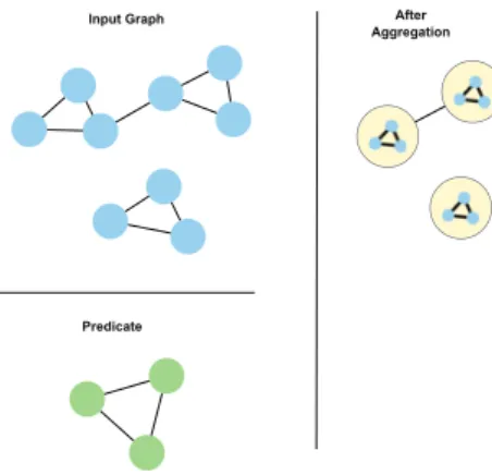
Example II.20. (Element aggregation by structure) In Figure 2.10 there is an input graph containing three triangular structures. An element aggregation by structure given the predicate shown will create three merged nodes. The two merged nodes that are connected to each other result from the connection between two of the triangular structures in the input graph. In the “after aggregation” picture, we can see the merged triangular structures within the new nodes. Figure 2.11 shows how the merged structures within the new nodes are stored. This is done by creating a model witness for the predicate. The new nodes point to the model witness structure.

2.5.3 Labeling function

Just observing a network can lead to many mental notes. But for every observa-tion, it is too cumbersome to open a new branch of analysis. In terms of our algebra,

(40)

Figure 2.10: After an element aggregation by structure, the attributed graph becomes only three nodes.

Figure 2.11: The three aggregated nodes in the merged graph of Figure 2.10 point to a model witness. The purpose of this model witness is the retain the predicate structure, the reason for the aggregation, to understand the analytical process.

(41)

we may prefer not to have to perform a selection and aggregation to create a new graph. Sometimes, simply making a note on the current graph will suﬃce. Then as analysis continues, these notes could be saved and easily tracked. The structure of this “mental note” on a graph leads us to our next operator: Labeling.

Labeling does not create a new graph, but it creates structured attributes based on a process similar to the element selection. The inputs to the labeling function are a set of attributed graphs and a predicate.

As a result of labeling, the attributed graphs that contain a witness are modiﬁed to include edges to a model witness (for the predicate). The model witness, similar to element aggregation, is given a new group id. This group id is used to identify it as an informational structure within the graph (not to be included in selections).

Below is a formal deﬁnition of labeling:

Definition II.21. (Labeling) Given a collection of n graphs and their attributes D, and predicate α = (Vα,Eα,XVα, XEα, XGα), a labeling, σ

label

element,α(D) is: For each

attributed graph Di in D where there exists a witness for the predicateα,

1. Create the model witness structure X withinDi

2. Label X’s nodes and edges with a unique group id (can be user deﬁned) 3. For each witness Wj found inDi use the mapping lists to create directed edges

from the nodes in Wj to the nodes X. For the new edges created in Wj to X

create two attributes: one to denote that it is part of one witness structure and another for the unique group id of this model witness.

Example II.22. In Figure 2.8, we show how to create new graphs based on an input set and predicate after applying the element selection operator. Sometimes an analyst

(42)

Figure 2.12: A labeling function performed on the same input graph and predicate from the element selection example, Figure 2.8

does not want to continually create more networks, rather within an exist network make notes and follow certain nodes of interest.

In Figure 2.12 we show how the labeling operator achieves this goal. Given the same input graph set and predicate from Figure 2.8, the result of the labeling operator is a model witness included into the graph (for the given predicate) and directed edges between the matched components of the input graphs. The model witness is not included in graph matching steps.

2.5.4 Visualization function

Preceding sections dealt with graph data manipulation and management. In Vi-sual Analytics, the viVi-sualization is a central step in relaying the results to the human analyst. Therefore, to complete the Graph Visual Analytic Algebra, a visual operator is needed to connect the data manipulation to the analyst. There are limitless vi-sual encoding and rendering expressions. The challenge is to create a vivi-sual operator without limiting possible visual expressions of information.

In an eﬀort to make this a systematic process, we break down the components of a visual function. A visual function, V, is described by an input predicate, a static visualization output, and a visual rendering/encoding mechanism. In this section, we

(43)

discuss the visual function and show an example of its use.

2.5.4.1 Visual function: Inputs, Visual Mechanism, and Outputs

The inputs to the visual function come from the graph data. Also, they can be represented as predicate form. The output is a static visualization. The “between” step, that we call the Visual Mechanism, processes data to produce the visualization output.

The following are a couple examples of what could be a Visual Mechanism:

• Diﬀerent layout options (force directed, circular, etc...) to display a graph Michailidis (2006)

• Coloring nodes by a rainbow gradient based on their degree value

Anything that results in a change on a display is fair game for the Visual Mech-anism. What exactly happens at this stage is a combination of computation and visual encoding/rendering. The computational part is a set of composition functions and attribute creations on the graph. The visual rendering and encoding depends on software and hardware restrictions.

2.5.4.2 Cytoscape Visual Display

A common visualization to create is coloring nodes on a rainbow gradient to show how an attribute value (in this case degree) varies on the graph. In this example, we show how this visual task occurs within a visual function in Cytoscape.

The input to the visual function is the phone data set from the VAST 2008 Chal-lenge (Grinstein et al.(2008),Shaverdian et al.(2009b)). The visual output we want to produce is a graph with its nodes colored based on their degree values.

The ﬁrst step is to create the degree attribute on each node. We follow the composition function technique from Example II.2 to create the degree attribute.

(44)

In Cytoscape, this visual task corresponds to selecting a continuous color mapping on the degree attribute, Figure 2.13.A. Within the algebra, for each node we create a color attribute with a value that maps to its color gradient (computed through a mapping composition function). The algebra could create an attribute to characterize all the visual encoding and rendering features, but to keep this example brief we only mention the degree and color ones.

Next the visual encoding and rendering will produce the output. Since we cannot bound the software and hardware possibilities for different tools, within the algebra we note this as a T ool Specif ic step. This step can be filled in with formalisms and languages that capture visual rendering specifics. Finally, the output layout is produced, Figure 2.13.B. In summary, this visual task corresponds to the following algebra:

1. Start: Vinput {P honeDataSet1}

A visual function is called on PhoneDataSet1.

2. Dphones = {G = (V, E), X = (XV = Xphone id, Xdegree, Xcolor, XE = (Xdate,

Xduration,Xtower, Xdirection of call),XG = ())}

After the user selects a mapping of color to degree, this color value is stored into Xcolor, a new node attribute.

3. V {T ool Specif ic}

A software process is run to produce the visualization output.

4. Complete: Voutput → Display

The visual function has completed with a display produced.

Setting a visual task into an algebra operator helps maintain the display infor-mation. In isolation, it seems like we took a simple visual task that might take an analyst a couple minutes to perform and turned it into a convoluted set of algebraic

(45)

A

B

Figure 2.13: A continuous color gradient mapping to node degree is set on the phone data set from the VAST 2008 Challenge.

expressions. But actually it becomes even more convoluted if there is no algebra to track visual tasks. If several different visual tasks are completed to reach an analyt-ical decision, it becomes difficult to replicate or verify the decision if the process is not documented. Also without using an algebra, as we discussed in the Introduction, comparing different tools and methods is difficult. Additionally, the visualization be-comes more flexible. By breaking down the visualization task, we can change points of the task, and mix and match with different methods. For example, we can rerun this current example on a new graph by simply modifying the input.

2.6 Implementation Example in Cytoscape

In this section we utilize Cytoscape and various plugins to show how the theoretical concepts presented in the algebra are realized in a practical analytical tool.

2.6.1 Graph Model

Currently we have described the graph model that is composed of the graph, the attributes, and composition functions. Cytoscape already provides a lot of the implementation to display the model. Figure 2.15 shows a Cytoscape display window after some networks have been uploaded. The networks we have uploaded are from

(46)

Figure 2.14: As part of our Visual Analytic Algebra, we deﬁne attributes as either computed or intrinsic. To allow the user to modify the type of an at-tribute we provide the following tab under the Control Panel. The user can view the attribute labels for nodes, edges, and the graph. To change the type from intrinsic to computed, the user can drag the attribute label from one type to another.

the VAST 2008 Challenge Data Set. The left panel shows the Control Panel. The Control Panel has several tabs.

We have installed two plugins, Visual Analytic Algebra and NetMatch. These plugins have added extra tabs to this panel that we will introduce throughout the paper. The Network Tab displays a list of network names. The Modify Attribute Types Panel, shown in Figure 2.14, displays the attribute labels for graph, edges, and nodes. In this panel, the type of the attribute can be switched from intrinsic to computed type.

2.6.2 Predicate Language

Again we use Cytoscape to place a real analytical setting for some of the theoretical ideas presented in the previous subsections.

We illustrate a predicate with the NetMatch Query Editor. Using NetMatch, an analyst can draw a new predicate and place conditional values on its attributes. Figure 2.16 displays the NetMatch Query Editor.

(47)

Figure 2.15: The main Cytoscape window is shown. There are three main components to its design. The network panel displays the network. The data panel displays node and edge specific attribute information. The control panel has several tabs to perform different functions on the network. One of these tabs is the network tab, that shows all the networks opened during a current Cytoscape analysis session. It allows the user to switch between different networks by saving them under different names.

Figure 2.16: The plugin NetMatch allows a user to draw a query. In essence, a query is a predicate. Attribute conditions are possible on nodes.

Query to NetMatch” button. This procedure will produce witnesses, as shown in Figure 2.17. Each witness will be displayed on its own row. The columns indicate the number of matches, the nodes that produced the match (corresponding to the mapping list), and an image of the witness.

(48)

Figure 2.17: Using the NetMatch plugin, we show the result of matching the input graph and the predicate shown in Figure 2.5. The image shown is a witness found in the input graph. The Node column shows the mapping between the witness and the predicate. This ﬁgure is an example imple-mentation of the Predicate, Witness, and Graph Matching features in the Visual Analytic Algebra.

2.6.3 Selection

We implement a direct way to perform set and element selection in Cytoscape through the Visual Analytic Graph Algebra Plugin. Under the Control Panel, the Operators tab has options to select a set of networks, the predicate, and operator to perform. Figure 2.18 this panel.

After a set selection has been applied on a set of the Phone Call Days data set from the VAST 2008 Challenge, the results are shown in Figure 2.19. The networks that satisfy the predicate are maximized and shown in the display panel. The networks that do not satisfy the ﬁgure are minimized in the background of the display panel.

To do an element selection, we use the same Operator tab. Figure 2.20 shows (1) the input graph, (2) the predicate, and (3) the results from element selection. As with a set selection, the analyst needs to ﬁrst specify an input graph and predicate. Element selection then utilizes the graph matching function to produce results. Three witnesses are found that match the predicate. The analyst can then create new networks for the witnesses found by selecting the witness and checking ”Create a new child network.” The match information can be saved for future use.

(49)

Figure 2.18: The Visual Analytic Graph Algebra Plugin also includes an Operators Tab in the Control Panel. Here the analyst can select a set of networks, the predicate list, and the operator to apply to the graphs. In this ﬁgure, the set selection Operator has been selected with the Predicate from Figure 2.1.

Figure 2.19: This ﬁgure shows an example implementation of set selection in Cy-toscape. Once the ”Done” button has been clicked, the result of the set selection is the set of graphs that satisfy the predicate are opened and displayed in the Display Panel. In this ﬁgure, four graphs are displayed.