Središnja medicinska knjižnica
Kalinić H., Lončarić S., Čikeš M., Miličić D., Bijnens B. (2012)
Image
registration and atlas-based segmentation of cardiac outflow velocity
profiles.
Computer Methods and Programs in Biomedicine, 106 (3). pp.
188-200. ISSN 0169-2607
http://www.elsevier.com/locate/issn/01692607
http://www.sciencedirect.com/science/journal/01692607
http://dx.doi.org/10.1016/j.cmpb.2010.11.001
http://medlib.mef.hr/1702
University of Zagreb Medical School Repository
http://medlib.mef.hr/
Image Registration and Atlas-based Segmentation of
Cardiac Outflow Velocity Profiles
Hrvoje Kalini´c1∗, Sven Lonˇcari´c1, Maja ˇCikeˇs2, Davor Miliˇci´c2, and
Bart Bijnens3
1 Faculty of Electrical Engineering and Computing, Department of Electronic Systems and
Information Processing, Universiy of Zagreb, Unska 3, 10000 Zagreb, Croatia (∗e-mail: [email protected])
2 Department for Cardiovascular Diseases, University Hospital Centre Zagreb, 10000
Zagreb, Croatia
3Catalan Institution for Research and Advanced Studies (ICREA) and Universitat
Pompeu Fabra (CISTIB), E08003 Barcelona, Spain
Abstract
Cardiovascular disease is the leading cause of death worldwide and for this reason computer-based diagnosis of cardiac diseases is a very important task. In this article, a method for segmentation of aortic outflow velocity profiles from cardiac Doppler ultrasound images is presented. The proposed method is based on the statistical image atlas derived from ultrasound images of healthy volunteers. The ultrasound image segmentation is done by registration of the input image to the atlas, followed by a propagation of the segmentation result from the atlas onto the input image. In the registration process, the normalized mutual information is used as an image similarity measure, while optimization is preformed using a multiresolution gradient ascent method. The registration method is evaluated using an in-silico phantom, real data from 30 volunteers, and an inverse consistency test. The segmentation method is evaluated using 59 images from healthy volunteers and 89 images from patients, and using cardiac parameters extracted from the segmented image. Experimental validation is conducted using a set of healthy volunteers and patients and has shown excellent results. Cardiac parameter segmentation evaluation showed that the variability of the automated segmentation relative to the manual is comparable to the intra-observer variability. The proposed method is useful for computed aided
diagnosis and extraction of cardiac parameters.
Key words: Doppler ultrasound imaging, cardiac outflow velocity profile, image registration, atlas-based segmentation, segmentation propagation
1. Introduction
At the beginning of the 20th century, cardiovascular disease was responsible for fewer than 10% of all deaths worldwide. Today, that figure is about 30%, with 80% of the burden now occurring in developing countries [1]. In 2001, cardiovascular disease was the leading cause of death worldwide [1]. In United States, coronary heart disease caused 1 of every 5 deaths in 2004 [2]. Therefore, one can conclude that diagnosis of coronary heart disease is a very important medical task.
In everyday clinical practice, a detailed analysis of Doppler echocardiography traces is often limited by a high frequency workflow in the echocardiographic laboratory. Currently, basic measurements of aortic outflow Doppler traces are routinely obtained by manual tracking of Doppler traces, predominantly provid-ing data on valvular flows. Manual trackprovid-ing of the traces is often cumbersome, time-consuming and dependent on the expertise of the cardiologist/sonographer. However, automatic trace delineation should reduce the required time needed for data analysis, while not increasing the measurement error. Previous clinical studies have demonstrated that additional data obtained by automatic trace analysis would provide relevant clinical data on left ventricular function, aiding in diagnostics and further patient management strategies [3, 4]. Continuous wave Doppler outflow traces are mainly used to assess a potential pressure gra-dient across the aortic valve resulting from a narrowing of the valve. It was also shown that severe aortic stenosis shows not only higher but often also prolonged outflow velocities [5]. The detection of changes in myocardial contractility in the setting of coronary artery disease is an important diagnostic task. Besides a decrease in global systolic function, as detected by ejection fraction, and changes in regional deformation [6], it was suggested, from isolated myocytes research,
that chronic ischemia decreases but prolongs contraction [7]. These observations show that the profile of the aortic outflow velocities might provide information on global myocardial function [8].
Ultrasonic imaging is a non-invasive medical imaging modality, which is routinely used in hospitals for the examination of cardiac patients [9]. Doppler ultrasound imaging provides useful information about blood velocities through the cardiac valves [10]. By measuring these velocities, clinical information on left ventricular (LV) inflow (mitral valve) and outflow (aortic valve) can be quanti-fied, which is clinically useful to assess hemodynamic parameters and ventricular function. The interpretation of Doppler echocardiography data requires an in-tegration of various hemodynamic measurements that can be obtained from the shape of the cardiac outflow velocity profile. To extract the information from the cardiac outflow velocity profiles acquired by the Doppler ultrasound, image segmentation and quantification of the segmented profiles is required. Both seg-mentation and quantification are usually done manually by expert cardiologist. However, manual segmentation of the images is usually a time consuming and tedious task. Cardiac Doppler ultrasound images are not exception from that. Since automating the segmentation and parameter quantification procedure has great potential for reducing the time cardiologist needs to spend to analyze each of the images, a new method for registration of aortic outflow velocity profiles is developed and presented in this paper. Within the registration procedure, a geometric transformation function is described which is specially developed for this type of the images. Also, a new atlas-based segmentation method is proposed, for automatic segmentation of cardiac outflow velocity profiles.
The atlas-based segmentation of aortic blood velocity profiles proposed in this paper, is a prerequisite useful for the quantitative analysis of coronary artery disease and aortic stenosis, such as the one described in [8, 3]. However, the motivation of this work is not only to solve the problem of the aortic out-flow velocity profile registration, but also to present a more general approach for registration of other cardiac images such as mitral valve velocity profiles. Furthermore, the proposed method for registration of the cardiac velocity
pro-files sets a framework for atlas construction, which can be used for statistical measurements of the population and for atlas-based image analysis. The seg-mentation of velocity profiles may also be used for signal feature extraction for statistical measurements of variability within population and for classification of velocity profiles into various classes.
2. Background
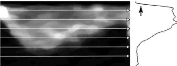
To the best of our knowledge there are no studies on the analysis of blood flow velocity profiles obtained by Doppler ultrasound published in literature, apart from the works of Tschirren et al. [11] and Bermejo et al. [12]. Tschirren et al. presented an automated cardiac cycle and envelope extraction of brachial artery flow profile based on image processing operations such as thresholding and correlation. However, this approach is not suitable for the cardiac outflow profiles mainly because it also segments the valve clicks (see Figure 2), not just the blood outflow. The work of Bermejo et al. analysed outflow profiles that are averaged and manually segmented, with a goal to analyse the valvular dynamics, so this work uses both a different methodological approach and a different hypothesis.
On the other hand, the published research on image registration [13] and seg-mentation [9] techniques is rather extensive. Since various information from im-age data is exploited to drive the imim-age registration algorithms, we can classify registration algorithms according to the information content used in registration into algorithms using designated landmarks [14, 15], contours [16] and surfaces [17] or various pixel properties functions [18]. The method proposed in this paper is based on the normalized mutual information (NMI) image similarity criteria [19, 20, 21] and a specially formulated geometrical transformation.
In [9] segmentation techniques are divided in low-level segmentation tech-niques (described in [22]) and high-level techtech-niques, where as a major difference between them is the level of the a priori information used in the process of segmentation. Although the low-level methods have shown some results on this
topic [23], experts usually rely on their experience to produce even better results. To develop a knowledge-based technique and incorporate a domain knowledge various models are used, such as statistical or artificial models based on an expert knowledge. Using a model, experimental data obtained from different subjects are easier to interpret. Preliminary results of using an image from a normal patient as a model are described by Kalini´c et al. [24]. The models with a common anatomical substrate are in medical applications often known as atlases. Atlas incorporates useful prior information for segmentation and registration tasks, so variation within population can be described with fewer (transformation) parameters. Atlases have broad application in medical image segmentation and registration and are often used in computer aided diagnosis to measure the shape of an object or detect the morphological differences be-tween patient groups. Various techniques for atlas construction are developed for different human organs, like the heart [25, 26, 27] and especially the brain [28, 29, 30, 31, 32, 33, 34, 35, 36, 37]. In this paper we use a statistical model as an atlas and an in-silico phantom model for evaluation. The atlas is the mean image, which is an estimate of the statistical expectation of the random field respresenting healthy volunteers.
3. Design considerations
In the rest of this paper, the registration algorithm and atlas construction are described in order to illustrate the atlas-based segmentation of aortic blood velocity profiles and followed by the experimental results. Since the inherent problem of the segmentation validation is the difficulty of obtaining the reliable reference, several validation techniques are used. The experiments can broadly be divided in two major groups of registration and segmentation validation.
The registration is evaluated using an in-silico phantom image, deformed real images, and inverse consistency criteria. The in-silico phantom was used so to have the known and reliable ground-truth. The arbitrary deformed real image can be used for the registration evaluation if the manually segmented
original (non-deformed) image is used as a ground-truth. Finally last criteria in the registration evaluation process was the inverse consistency as proposed by Christensen et al. [38] and Lorenzen et al. [32].
The segmentation is evaluated on 59 images from healthy volunteers and 89 images from patients, using manual segmentation by an expert cardiologist. In this way the segmentation is tested on the set of images which are anatomi-cally far from the atlas, since only the healthy volunteers were used for atlas construction. To check the usability of the proposed segmentation in clinical practice, several cardiac parameters with diagnostic potential are extracted from atlas-based segmentation and ground-truth segmentation. When compared to intra-observer variability these parameters also show the segmentation accuracy.
4. Method
This section presents the proposed method for atlas-based segmentation. In atlas-based segmentation, the input image is registered to the pre-segmented atlas image. The registration result returns the parameters of geometrical map-ping from the input image onto the atlas image. With the inverse geometrical mapping the segmentation from the atlas is propagated on to the image. In the following text, the input image will be referred to as the source image and the atlas image will be referred to as the reference image.
The images used in this study are the aortic outflow profiles obtained using continuous wave Doppler mode. All the images were acquired by echocardio-graphic scanner (Vivid 7, GE Healthcare) using an apical 5-chamber view. Im-ages were digitally stored in ’raw’ Dicom format, containing the spectral Doppler information in proprietary tags. These ’raw’ Dicom images were converted into Hierarchical Data Format (HDF) using an Echopac workstation (GE Health-care). From the input HDF file, the image containing information about aortic flow, was extracted. An example of this image is given in Figure 1.
In the following sections a new registration algorithm, composed of a geomet-ric transformation, similarity measure and optimization algorithm is described.
Figure 1: An example of the image extracted directly from the HDF file.
Next, the method for creation of a statistical atlas image, that is used as the reference image, is proposed. The reference image is manually segmented by an expert cardiologist and the result is mapped to the input image to provide the segmentation result. At the end of Section the atlas-based segmentation procedure is described.
4.1. Registration
The goal of image registration is to determine parameters of the geometric transformation, that maps a source image into a reference image. The images that need to be registered are denoted as S(x) and R(x), where the sets of pixels of these images are {S(i)} and {R(i)}, respectively. The image S(x) is the source image and S0(x) denotes the transformation of the image S(x) (i.e. S0(x) = S(T(x))) obtained by the successive estimate of the registration transformationT. The imageR(x) will be treated as the reference image. Thex
will be used to denote vector defined by the ordered pair in Cartesian coordinate system (t, v), since Doppler ultrasound images represent the instantaneous blood velocity (v) within the sample volume (pulsed Doppler) or scan line (continuous wave Doppler) as a function of time (t).
The registration method consists of transformation and optimization with respect to the defined similarity measure. Detection of the ejection time interval is performed manually based on two points in time. Detection of low velocity region is done automatically. This information is used for an initial alignment
of the images. Manual selection of the ejection time interval requires about 2 seconds of time, which is negligible compared to the time required for manual profile segmentation which may last up to 60 seconds.
The rest of the registration procedure stretches the image along the velocity axis, in several bands, and is described in more details below. NMI is used as a similarity measure. The similarity measure is maximized using a modifica-tion of the gradient ascent optimizamodifica-tion algorithm. This secmodifica-tion is divided into three subsections dedicated to the major parts of the registration procedure: transformation, similarity measure and optimization algorithm.
Figure 2: The outflow velocity profile from a healthy volunteer. The low velocity region is marked with the black ellipse, and the valve clicks which define the relevant part of the phase cycle are marked with arrows at the bottom of the figure.
4.1.1. Transformation
After the relevant phase of the cardiac cycle is extracted as described in [23] and all images are aligned, the transformation functionT, in general case, can be written as: T(t, v) = [ e(t, v) 0 0 f(t, v) ] · [ t v ] (1) wheree(t, v) andf(t, v) are arbitrarily function of time and the velocity.
After resizing all the images to the same resolution, phases of all outflow velocity profiles are matched. Now, no transformation intdimension is required, therefore we set e(t, v) = 1. All the possible inter-individual changes in the profiles can now be governed only by the variablef(t, v) from the Equation 1,
which we call the scaling function. It is important to notice that the scaling function is a function of time, i.e. f(t, v) = f(t). Now, we have the scaling function that can be used to quantify the instantaneous blood velocity change for different outflow profiles.
For practical reasons, a parametrized scaling function is used. The function is parametrized by selecting N equidistant points, which are sorted in a row vector. The vector is denoted asfand will be addressed as the transformation vector. This can be written as follows:
ti =
(i−1)·P
N−1 ,∀i= 1, .., N fi = f(ti)
f = [f1...fN] (2)
where P stands for phase cycle of outflow velocity profile. Now, the transfor-mation of an image is described and quantified with the transfortransfor-mation vector components. The reconstruction of a scaling function from the transformation vector is done using linear interpolation. If one selects N = 11, as we did in this study, the image transformation and the transformation vector components can be visualized as depicted in the Figure 3, where white circles represents the transformation vector components, and the curve interpolated between them represents the interpolated scaling function (f(t, v)).
Figure 3: The original image (left) and the transformed image with transformation vector components (right).
It is also important to notice that since the transformation function is parametrized and has N degrees of freedom, the optimization space is N-dimensional. The details of the optimization algorithm are described further
in the section 4.1.3. In the next section, we will first discuss the similarity measure.
4.1.2. Similarity measure
If the similarity measure between images S(x) and R(x) is denoted as E(S(T(x)), R(x)) the images are optimally registered (with respect to given-similarity measure and degrees of freedom) when the maximum of the function E is achieved:
Toptimal= arg max
T E(S(T(x)), R(x)) (3)
Clinically obtained aortic outflow velocity images sometimes differ signifi-cantly, resulting in low (local) correlation and different resolutions with differ-ing texture. Additionally, Doppler ultrasound images inherently contain a lot of (speckle) noise. To register this kind of images it is necessary to find a simi-larity measure that does not make any assumptions regarding the nature of the relation between the image intensities (see also [21] and [19]).
As a solution, the mutual information is used in its normalized form [21]: N M I(S, R) =H(S) +H(R)
H(S, R) (4)
since it overcomes many of the shortcomings of joint entropy and is more robust than mutual information (MI) [39, 20]. HereH(S) andH(R) denote the entropy of imagesS andR, andH(S, R) the joint entropy.
It is important to notice that the similarity measure is not calculated for the set of pixels in the overlapping region ofR and S0, i.e. withinC =R∩S0, as assumed in [39]. Instead, it is calculated for all pixels in the reference image except for the low velocity region (see Figure 2). The region over which the NMI is calculated may be written as
D=R\({S0(i)} ∪ {R(i)}),∀i∈L (5)
whereL is the set of pixels from the low velocity region (both in imageS and R). Low velocity region is decided after projection of the image onto the y-axis
Figure 4: Region L is decided after projection of the image onto the y-axis. Black arrow indicates end of low velocity region.
as shown in Figure 4, as set of pixels having the projection lower than 10% of the projection maximum.
The reason not to calculate NMI over the regionCis becauseCis a function ofT, i.e. C=C(T), so to avoid influence of the transformation function on the similarity measure. The problem of non-existent values for the source image is solved as suggested by Roche et al. in [40]. In short, these values are artificially generated during the transformation, using the pixels from the image border.
4.1.3. Optimization Algorithm
The gradient ascent numerical optimization method is used to find the global maximum of the energy function. The pseudocode for this algorithm is given below, whereEstands for the energy function. The energy functionEis calcu-lated as the Normalized mutual information between two imagesS(T(x)) and R(x) (see Equation 4), over the regionD, as defined in Equation 5 and described in section 4.1.2. Same as above,f andN denote the deformation vector and its dimension.
Function gradient ascent(starting point, E) define: µ, γ, δ, tolerance
f=starting point
do
for i= 1 to N
sample E around fi with µ
approximate dE/dfi from sampled points
if dE/dfi> γi·δ
γi= 0.95·γi
end if end for
f=f+ 3·µ·γ·(dE/df)/norm(dE/df)
while norm(dE/df)> tolerance
return f
In this algorithm,δis an estimation of the optimization function gradient at the starting point (according to Fletcher [41]). The gradient has to be smaller for every next step to assure that the algorithm converges. This is done using γ, which modifies the convergence rate, forcing the change of f to be smaller for every next step.
Since Doppler ultrasound images contain a lot of noise, registration of these images is very sensitive to the initial conditions and the convergence step, and may easily end up in a local (instead of global) optimum. To assure the accuracy and robustness of the proposed method, a two-step multiresolution optimization approach is used. This approach is described in the pseudocode below.
Define S(−→x), R(−→x), starting point
Resize S(−→x) and R(−→x) to 100x100px Define f ilt= gaussian filter with σ= 9px Sb= convolution(S(−→x), f ilt)
Rb= convolution(R(−→x), f ilt)
Define E(−→f) =N M I(Sb(T(−→x)), Rb(−→x)) −
→
f1 = gradient ascent(E(−→f), starting point)
Define E(−→f) =N M I(S(T(−→x)), R(−→x))
− →
With this implementation of the multiresolution approach a trade-off be-tween speed and accuracy is made, since the images are not downsampled. The downsampling is avoided since it causes histogram changes, which in turn may cause some of the artefacts similar to the ones mentioned in [42].
4.2. Atlas Construction
The purpose of a statistical atlas is to combine many images into a single image, which represents a statistical average of all images. In this method, we have used the arithmetic image averaging operation to construct the atlas. After all aortic outflow velocity images are aligned and resized, the atlas is constructed as an average intensity atlas using the formula:
A(t, v) = 1 K K ∑ i=1 Si(t, v) (6)
where Si are the images used to construct the atlas. Using this approach the
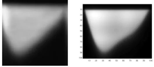
atlas image fromK = 59 images from 30 healthy volunteers is constructed for the purpose of this study. The resulting image is shown in Figure 6 (left).
4.3. Atlas-based Segmentation
The idea of atlas-based segmentation is based on the use of a representative reference (or atlas) image, where the desired structure is manually segmented by an expert cardiologist. In our case, the desired structure is the aortic outflow velocity profile. Expert segmentation is done only once, and is later automati-cally propagated to the other images of this type. When a new patient image is acquired, the segmentation is conducted in four steps:
(a) The new image that needs to be segmented is declared as a source image. (b) The source image is registered to the reference image, resulting in a set of
parameters describing the geometric transformation.
(c) The segmentation of an aortic outflow profile from the reference image (the atlas) is propagated to the source image.
(d) The source image along with the propagated segmentation is backward transformed (using the inverse set of parameters) to its original form.
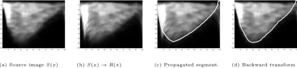
This procedure is depicted in Figure 5 where each step is represented with one image. As the reference image, the manually segmented atlas is used.
(a) Source imageS(x) (b)S(x)→R(x) (c) Propagated segment. (d) Backward transform
Figure 5: The segmentation procedure: Each image represents one step described in Section 4.3. All axis are in pixels.
5. Experiments and Results
This chapter is focused on evaluating the registration algorithm accuracy and the comparison of atlas-based segmentation with the segmentation done by an expert cardiologist. First, the registration validation using an in-silico phan-tom, along with the phantom construction, is presented. Second, the validation on real data is presented, where the exact geometrical transformation between data sets is known. Third, the validation of the registration accuracy on a set of test data based on inverse consistency is presented. Fourth, the atlas-based segmentation is validated on 59 images from healthy volunteers manually seg-mented by an expert cardiologist. Fifth, the same segmentation validation is done on 89 images from patients with a diagnosis of either coronary artery dis-ease or aortic stenosis. Sixth, the segmentation is validated by comparison of the cardiac parameters extracted from the manual and automated segmenta-tion. Finally, intra-observer variation is studied and compared with the error between manual and automated segmentation.
5.1. Phantom study-based registration validation
The outflow velocity is modeled using a linear combination of sinusoidal functions. The attenuation is modeled by an inverse tangent function:
wherec1,c2andc3 are constants used for centering the image on the coordinate
system, andF(x) is constructed as:
F(t) =sin(πt) +sin(2πt)
4 +
sin(3πt)
6 (8)
The attenuation of low blood velocities is modeled similar to eq. 7 using the function:
A(v) = 1
π·arctg((v−a1)·c4) +c5 (9)
The parameter a1 can be used to set the percentage of the outflow velocities
that will be attenuated, in our case it is set to 10%. The resulting image is shown in Figure 6.
Figure 6: The average intensity atlas (left) and the phantom image (right)
To validate the registration accuracy on the phantom image, the source and reference image have to be defined. Part of the registration error is due to the suboptimal performance of the optimization algorithm and the properties of the similarity measure. This error can be quantified if the desired transformation is known. For this reason the following experiments are constructed. An image with different velocity outflow profile shape is constructed from the phantom image using a random transformation. Random transformation is here defined by a transformation vector, whose eleven elements are picked from the uni-form distribution on the interval [0.7,1.4]. Using the random transuni-formation, 50 variations of the phantom image are constructed.
In the first experiment the original phantom is selected as a source image and the deformed phantoms as reference images. Here, the goal of the registration
algorithm is to reconstruct the deformation function. The registration error can now be calculated as difference between deformation and the transformation as found by optimization algorithm. Since the transformation is parametrized by the transformation vector this reduces to:
e1=kf1−f2k2 (10)
wheref1andf2are row vectors which represent respectively random deformation of the phantom image and the deformation approximation as found by the registration algorithm. The average error vector components from 50 different phantom transformations equals to µ(e1) = 1.68% with standard deviation of σ(e1) = 0.92%.
In the second experiment, the original phantom is labeled as reference image and the deformed phantoms as source images. Now the registration algorithm has to find the inverse transformation function. For each pair of images the registration error is calculated using the Equation:
e2=k1−f1·f3
Tk
2 (11)
where f1 and f3 are row vectors, which represent the random deformation of the phantom image and the inverse, as found by the registration algorithm. Same as before, the mean error vector components and their standard deviation are calculated. Mean error is µ(e2) = 2.15% and standard deviationσ(e2) = 1.92%. One may notice that the error and deviation is smaller in the first experiment, which is due to the direction of the registration algorithm. In the first experiment the registration algorithm searches for the transformation parameters in the same direction that is used for the deformation, while in the second experiment the opposite direction is used (i.e. in this experiment the deformation model is not the same as the transformation function).
5.2. Real image-based registration validation
The similar experiment, as the one explained above on the in-silico phantom image, is conducted on real images of cardiac aortic outflow velocities. This
was done since the phantom image used in previous section does not have any (speckle) noise, does not model valve clicks and small deviations of the time frame which are possible to show up in the real images. In this experiment, from a set of 59 images, each was deformed with thirty random transformation vectors and the registration algorithm searched for vectors that will re-transform these images back to their original form. The vector elements used for the deformation are randomly picked from the uniform distribution on the interval [0.7,1.4], and the starting vector for the optimization algorithm is the unity vector. The error vector is calculated using the equivalent formula as in Equation 11 and denoted as e3. In this experiment the average error is µ(e3) = 2.93% with standard deviation ofσ(e3) = 2.03%.
5.3. Inverse consistency-based registration validation
The final registration experiment is based on the inverse consistency test. Although inverse consistency does not guarantee the accuracy of the registra-tion, it is often preferable or even used as measure of quality of the registration [38, 32]. This, along with the desire to quantify the bi-directional transforma-tion error, are the main reasons for the additransforma-tional validatransforma-tion using the inverse consistency test [43, 44]. Each of the images from the set is registered to all the others images from the set. In this way, the registration is done bi-directionally (i.e. the imageI1s registered to imageI2and vice-versa). Using the notation.∗
for Hadamard product (where only the corresponding vector elements are mul-tiplied) andf(I2, I1) for the transformation vector received after registration of
imageI1 to imageI2, the mean error vector is calculated as:
e4= 1 N N ∑ i=1 |1−(f(i)(I2, I1).∗f(i)(I1, I2))| (12)
whereN represents the total number of registration experiments. If the number of images isnthen the total number of registration experiments equals toN =
n2+n
2 , since registration of an image onto itself is also taken into account. The
5.4. Atlas-based segmentation validation: Healthy volunteers
The atlas-based segmentation validation is done on 59 outflow profiles from 30 healthy volunteers. The expert manually segmented the atlas image (con-structed as described in section 4.2), and this atlas is used as a template for the segmentation.
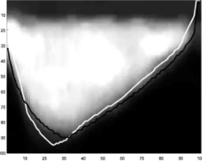
Figure 7: The comparison of manual (black) and propagated (white) segmentation. Both axes are in pixels.
Figure 8: Propagated segmentation with small deviation of automated segmentation (white) from the manual segmentation (black). Both axes are in pixels.
With the procedure as described in section 4.3 the manual segmentation is propagated from the atlas image to the rest of the 59 images. These images are compared with the ones that are segmented manually by the same cardi-ologist. For the brevity of the presentation, only some of the results, that are
Figure 9: Propagated segmentation with larger deviation of automated segmentation (white) from the manual segmentation (black). Both axes are in pixels.
Figure 10: The comparison of manual (black) and propagated (white) segmentation on the outflow profiles with the starting valve click. Both axes are in pixels.
representative of all results, are presented. These images are shown in Figures 7, 8, 9 and 10. In Figure 7, we may see the manual and the automated segmen-tation results that correspond very well. In Figure 8 we want to point out the small bumps that exist in the automated segmentation, while there is no trace of them in the manual segmentation. Although, the automated segmentation corresponds well to the manual segmentation, the bumps may be explained as an inherent intensity change. If we take a look at the Figure 9 we may no-tice that, around the peak, the automated segmentation peaks over the manual segmentation. Nevertheless, this segmentation result explains well the shape of
the signal despite the selection of a different threshold. In the Figure 10 the outflow profiles with the starting valve click is shown. In clinical practice, the cardiologists try to distinguish between the blood flow and the valve click based on their experience, since only the blood flow bears significant information for diagnosis. It can be seen how the manual segmentation performs across dif-ferent intensities, as if there is no valve click. When this is compared to the automated segmentation there is a difference, but automated segmentation also managed to ignore the valve click. This last results (Figure 10) demonstrate also the important improvement compared to the work of Tschirren et al. [11] since these results cannot be reproduced using just envelope detection. When the numerical results of the manual and automated segmentations are compared, this knowledge from the visual inspection should also be taken into account, since it is disputable whether some of these errors are errors indeed. If manual and propagated segmentations are observed as sampled function and denoted as mi[t] and pi[t], respectively, wherei stands for the instance of the Doppler
outflow image, the error may be measured as average difference betweenmi[t]
andpi[t] and written as:
de= 1 K·M K ∑ i=1 M ∑ t=1 |mi[t]−pi[t]| (13)
whereK stands for the number of images, i.e. K= 59, and M for the number of samples in the time (phase) frame, i.e. M = 100. Using this measure we may say that the propagated segmentation deviates in average by 4.6 pixels from the manual. Since all the images have been resized to 100-by-100 pixels, images have 100 samples in the velocity direction and so do the functions mi[t] and
pi[t]. Since the transformation is done along th y-axis this error corresponds to
4.6%.
The sample correlation coefficient between manual and propagated segmen-tation of all outflow profiles is also calculated. This is done using the Equation:
r= 1 M−1 M ∑ t=1 m[t]−µm σm ·p[t]−µp σp (14)
Hererdenotes the sample correlation coefficient for one instance of the outflow profile, and M, m and p are used as defined above. The average sample cor-relation coefficient of the population isr = 0.98 with the population standard deviationσr= 0.024. The minimal and maximal sample correlation coefficient
between manual and propagated segmentation arermin= 0.86 andrmax= 0.99,
respectively, which shows excellent statistical correlation between manual results and the proposed method for atlas-based segmentation.
5.5. Atlas-based segmentation validation: Patients
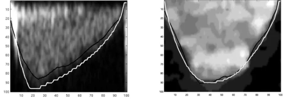
In the previous subsections, the validation is done on the aortic outflow profile that is either artificially created or belongs to the data set that is used to create the atlas. To validate the segmentation procedure on the outflow profiles from different data sets 89 outflow profiles are selected. 36 of these outflow profiles belong to patients with coronary artery disease (CAD) and 53 of them belong to patients with aortic stenosis (AS). Again, the manual segmentation is propagated from the atlas to all the instances of the patients outflow profiles as described in section 4.3. These images are compared with the ones that are segmented manually by the same cardiologist. In Figure 11, representative images of the patients with diagnosed CAD and AS are presented, with both manual and automated segmentation of the outflow profile.
Figure 11: The comparison of manual (white) and propagated (black) segmentation for pa-tients with diagnosed CAD (left) and AS (right)
If the same measurements as for normal patients are used (see Subsection 5.4), we can see that the average automated segmentation error with respect to the manual segmentation isde = 5.08% for the patients with diagnosed aortic
stenosis, andde= 8.70% for the patients with diagnosed coronary artery disease.
At the same time, the correlation coefficient between manual and automated segmentation isr= 0.98 both for the patients with AS and CAD. The maximum sample correlation coefficient isrmax = 0.99 for both set of patients, while the
minimum sample correlation coefficient isrmin= 0.96, for patients with CAD,
andrmin= 0.92, for patients with AS.
5.6. Cardiac parameter-based segmentation validation
In this subsection, we describe a segmentation validation procedure based on the comparison of the cardiac parameters extracted from two aortic out-flow profiles. The first aortic outout-flow profile is obtained by the proposed auto-matic segmentation method, while the second aortic outflow profile is obtained by manual segmentation. Cardiac parameters that are measured are: time to peak, peak value and rise-fall time ratio. These parameters have shown to have potential for use in diagnosis of some of the cardiac disease (see [23] or [8]), however, they are not routinely used in clinical practice since their extraction is often subjective, being both dependent on computer display (brightness and resolution) as well user interpretation, as will be shown in the next section.
Letttpm and ttpa denote time-to-peak values extracted by manual and
au-tomated procedures, respectively. Similarly, let the same notation be used for the maximum value and rise-to-fall-time-ratio parameters (maxm,maxa,trfm,
andtrfa). Since outflow velocity profiles belong to different patients, different
pacing and different velocities are expected. Therefore, to exclude the variation due to different patient characteristics and to observe the segmentation variation only, relative parameter errors are calculated and given as percentages rather than absolute values.
In this experiment, we calculate the relative error between the automated and manual segmentation, which in the case of time-to-peak parameter is
ex-pressed as:
ettp=
ttpa−ttpm
ttpm (15)
For comprehensive analysis of method accuracy we calculated three statisti-cal error measures: mean error, standard deviation of error, and mean absolute error. If a systematic error (bias) is present, it will be evident from the mean error and from the mean absolute error. Standard deviation of error does not detect systematic error. If no systematic error is present, then the mean er-ror will be equal to zero and hence is not useful for erer-ror evaluation. In this case, both standard deviation of error and mean absolute error can be used for accuracy evaluation.
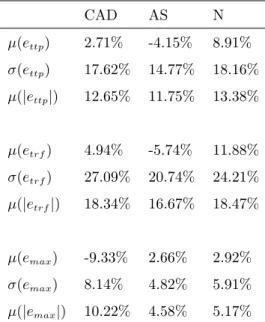
In Table 1 mean error, standard deviation of error, and mean absolute error of the observed cardiac parameters (automated vs. manual) are presented. The results from patients with diagnosed coronary artery disease (CAD), patients with diagnosed aortic stenosis (AS), and volunteers with normal outflow profiles (N) are given in separate columns.
It is evident from Table 1 that certain amount of systematic error exists. Standard deviation of error and mean absolute error are measures that show the amount of error, other than systematic error. The table shows that standard deviation of error and mean absolute error are highly correlated. Therefore, we can conclude that both measures can be used for evaluation of error.
For the interpretation of the results, one should note that the time to peak falls somewhere around the first quarter of the ejection time frame. For the images presented in this paper, that would be around 25 pixels. If e.g. time-to-peak parameter estimate is inaccurate by one pixel only this will result in 4% error. This can be observed on the Figure 11 (left) where the relative errors in terms of the cardiac parameters are: ettp = 16.28%, etrf = 21.71% and
emax = 10.74%; which are the values that are comparable with the standard
deviation of the relative error in Table 1.
In addition to error measures, we have calculated the correlation between cardiac parameters extracted from manual and automated segmentation. For
CAD AS N µ(ettp) 2.71% -4.15% 8.91% σ(ettp) 17.62% 14.77% 18.16% µ(|ettp|) 12.65% 11.75% 13.38% µ(etrf) 4.94% -5.74% 11.88% σ(etrf) 27.09% 20.74% 24.21% µ(|etrf|) 18.34% 16.67% 18.47% µ(emax) -9.33% 2.66% 2.92% σ(emax) 8.14% 4.82% 5.91% µ(|emax|) 10.22% 4.58% 5.17%
Table 1: Mean error, standard deviation of error, and mean absolute error between cardiac parameters obtained from manual and automated segmentation. Rows 1-3 show errors for time-to-peak parameter, rows 4-6 show errors for rise-to-fall-time-ration parameter, rows 7-9 show errors for peak-value parameter.
example, for the time-to-peak parameter the correlation is defined as: c(ttpa, ttpm) = ∑K i=1ttp a·ttpm √∑K i=1(ttp a)2√∑K i=1(ttp m)2 (16)
The results have shown a very high statistical correlation between the cardiac parameters extracted using our method and the cardiac parameters extracted by the expert cardiologist. For example when time-to-peak parameter is measured a correlation ofc(ttpa, ttpm) = 0.988 is achieved, for the rise-fall time ratio the
correlation is c(trfa, trfm) = 0.974, and for time to peak c(maxa, maxm) =
0.997.
5.7. Intra-observer variability
In the previous subsections, the proposed method is compared to an ex-pert manual segmentation. However, it is well known that there can be a con-siderable intra-observer and inter-observer variability of the results of manual
segmentation. The intra-observer error is the error between subsequent results of the segmentation of the same image performed by the same person. The inter-observer error is obtained when several different people segment the same image. Typically, the inter-observer error is larger than the intra-observer error. One must be aware of these errors when a manual segmentation by one or more expert cardiologists is used as a validation reference, as these errors limit the validation accuracy.
To quantify the intra-observer error the following experiment is conducted. An expert cardiologist segmented 21 images that she already segmented one week ago. If the segmentation results are observed as two sets of measurements, this gives a total of 2100 measurements (since images are resized to 100-by-100 pixels) for each set. If the measurementsm1(i) from the first set are interpreted
as realizations of the random variablem1 and the measurementsm2(i) from the
second set are interpreted as realizations of the random variablem2 then the
random variabledm defined as:
dm=m1−m2 (17)
describes the difference between the two measurements. Since we do not know which measurement is the reference one (which represents the correct segmenta-tion) we calculate the standard deviation as an estimate of the varianceσ2(d
m)
of the random variable and the mean absolute error (µ(|dm|)). Similarly, let
da = a−m be the random variable representing the difference between the
automated (a) and manual delineation (m). Since we had 59 images from vol-unteers, and 89 images from patients, this results in a total of 14800 random variables. The realizations of these two random variables are shown in Figure 12, withσ2(d
m) = 28.94 andσ2(da) = 47.51.
The mean absolute error between the automatic and the manual segmenta-tion is equal toµ(|da|) = 5.57px, while the standard deviation of the difference is
σ(da) = 6.89px. The mean absolute error between two different segmentations
of the same image made by the same cardiologist is equal toµ(|dm|) = 3.62px,
0 500 1000 1500 2000 2500 −60 −50 −40 −30 −20 −10 0 10 20 30 40 Error (d m )
Measurement number (i)
Figure 12: The upper graph shows the difference between two manual segmentations (intra-observer variability), while the lower graph shows the difference between manual and auto-mated segmentation.
variability of the difference between the automatic and manual segmentation is comparable to the intra-observer variability (6.89px vs. 5.38px).
The intra-observer variability of the cardiac parameter extraction is also calculated. To compare it with the results from Section 5.6, the standard de-viation of the relative time-to-peak error is calculated as in Table 1 and gives σ(ettp) = 11.91%, while the standard deviation of relative error of rise-fall time
ratio givesσ(etrf) = 16.28%. When we look at the standard deviation of
rela-tive peak value error, we can see that manual segmentation has a variability of σ(emax)) = 5.15%. If these results are compared with the rest of the results in
Table 1, we can see that the parameters from automated segmentation varies from the manual segmentation just slightly more than the manual
segmenta-tion from itself. The same is true if we observe the mean absolute error since µ(|ettp|) = 9.07%,µ(|etrf|) = 12.54%, and µ(|emax|) = 3.43%. While having in
mind these results and the high correlation between manually and automatically extracted parameters we conclude that one may use the proposed atlas-based segmentation for cardiac parameters extraction.
5.8. Statistical analysis of manual and automatic parameter measurement For statistical validation the automated and manual methods for parameter measurement, the t-test is used. Letea
param ande m
param denote the
automatic-to-manual error (error between automatic and manual parameter extraction) and manual error (human intra-observer error). The param in the subscript identifies which parameter is tested (ttp,trf or peak).
The proposed null hypothesis is: The mean values of the errorsea
param and
em
paramare equal i.e. the intra-observer parameter error is equal to the error
be-tween the automated and manual parameter extraction. The t-test allows a com-parison of two datasets with different numbers of samples. In this experiment the first dataset has 21 and the second dataset has 148 elements (Section 5.7). The t-test is performed using Satterthwaite’s approximation to calculate the number of degrees of freedom and without assumption of the same variability of both datasets (Behrens-Fisher problem). The p-values calculated from the t-test are given in Table 2.
ttp trf peak
p−value 0.6843 0.7398 0.3908
Table 2: The p-values for tome-to-peak, rise-fall-time-ratio and peak cardiac parameter.
The p-values for all three cardiac parameter errors (time-to-peak, rise-fall-time-ratio and peak value) are much above the traditionally used significance level (α) of 0.05. One rejects the null hypothesis if the p-value is smaller than or equal to alpha. Sinceα= 5% is much lower than the lowest p-value we may conclude that there is no statistically significant difference (at the 5% level)
between the datasets or that there is no enough evidence to reject the null hypothesis that the intra-observer parameter error is equal to the error between the automated and manual parameter extraction. As we can see, this is true for all the cardiac parameters evaluated in this paper.
6. Discussion and Conclusion
The main contribution to the current state of the art presented in this paper is the proposed atlas-based segmentation method, as the first fully automatic aortic outflow segmentation method presented in literature.
A comprehensive validation of the registration method is conducted using an in-silico phantom (Section 5.1), 59 outflow profile ultrasound images from 30 healthy volunteers (Section 5.2), and the inverse consistency test (Section 5.3). The exhaustive validation of the atlas-based segmentation is done with respect to an expert manual segmentation. First, the 59 outflow profiles form the healthy volunteers are segmented using the atlas described in Section 4.2 and segmentation described in Section 4.3. The validation is described in Section 5.4. Second, 89 outflow profiles from the patients are segmented using the same atlas and the same segmentation procedure and validated in Section 5.5. In both experiments the difference and correlation between manual and propagated segmentation is calculated. Third, the segmentation is evaluated based on the cardiac parameters extracted from the automated segmentation (Section 5.6). Finally, the results are compared to the intra-observer variability of the manual segmentation (Section 5.7 and Section 5.8).
The phantom validation demonstrated that the registration is quite accurate, with an error of the transformation vector around 2% (see Section 5.1), at the same time the validation on real images gives an error of the transformation vector of around 3% (see Section 5.2). A portion of the errors is due to the asymmetry of the forward and backward transformation as explained in Section 5.3.
compared to the manual segmentation by an expert cardiologist, the differ-ence, as an error measure of the automated segmentation, is 4.6%, on average. The correlation between the manual and automatic segmentation is on average r = 0.98. Thus, we may conclude that the proposed method for the image registration may be used for the automatic segmentation of Doppler ultrasound images. Additionally, due to the intrinsic properties of the method, the method handles the valve click correctly and therefore is especially valuable in the au-tomatic segmentation of the aortic outflow profiles.
The segmentation validation on the patients showed that the automatic seg-mentation with respect to the manual segseg-mentation differs by 5.08% for the patients with the diagnosed aortic stenosis, and 8.70% for the patients with the diagnosed coronary artery disease. For both set of patients the correlation of automated and the manual segmentation is around r = 0.98. All of this shows us that the proposed atlas can be used for the patients as well as for the volunteers.
The registration and segmentation results are condensed in Table 3. Validation type Error
Phantom 2.2%
Real images 2.9%
Atlas/volunteers 4.6%
Atlas/AS 5.1%
Atlas/CAD 8.7%
Table 3: Condensed experimental results. First two rows show the registration error (measured on synthesized examples), while the last three rows show the segmentation error (measured on empirical data).
If the standard deviation of the difference between manual and automated segmentation is calculated over the whole set (volunteers and patients) and com-pared to the intra-observer variability we can see that both errors have the same order of magnitude (Section 5.7). The same conclusion holds for the average of
absolute values, which is summarized in Table 4. In addition, Section 5.8 shows that there is no statistically significant difference between automatic-to-manual and manual (intra-observer) error. In this sense, we can conclude that the accu-racy of the method is fundamentally limited by the (in)accuaccu-racy of the manual segmentation. Comp-Human INTRA σ(ettp) 17% 12% µ(|ettp|) 12% 9% σ(etrf) 23% 16% µ(|etrf|) 18% 13% σ(emax) 6% 5% µ(|emax|) 7% 3%
Table 4: Standard deviation and average of absolute values of percentage difference between cardiac parameters from manual and automated segmentation.
As reported, the mean value of the absolute difference between the auto-mated and the manual segmentation is equal to µ(|da|) = 5.57px, while the
standard deviation of the difference isσ(da) = 6.89px. When this is compared
to the mean value of the absolute difference between two different segmentations of the same image made by the same cardiologist (µ(|dm|) = 3.62px) and the
standard deviation of the difference (σ(dm) = 5.38px) it is obvious that these
two segmentations are relatively close to one another. This is even stronger em-phasized when the correlation between cardiac parameter extracted from auto-mated and manual segmentation is observed since correlations for time-to-peak, rise-fall time ratio, and peak parameter are c(ttp) = 0.9875, c(tr/f) = 0.9741,
andc(max) = 0.9966, respectively. Therefore, we conclude that the proposed atlas-based segmentation has comparable accuracy and precision to a human expert.
7. Acknowledgements
This work has been supported by Ministry of science, education and sports of the Republic of Croatia under grant 036-0362214-1989 and by National Foun-dation for Science, Higher Education and Technological Development of the Republic of Croatia under grant ”An integrated, model based, approach for the quantification of cardiac function based on cardiac imaging”.
The authors would like to thank the anonymous reviewers for their valuable comments.
8. Conflict of interest
None declared.
References
[1] T. A. Gaziano, Cardiovascular Disease in the Developing World and Its Cost-Effective Management, Circulation 2005 (2005) 3547–3553.
[2] A. H. Association, Heart Disease and Stroke Statistics - 2008 Update (2008).
[3] M. Cikes, H. Kalinic, A. Baltabaeva, S. Loncaric, C. Parsai, D. Milicic, I. Cikes, G. Sutherland, B. Bijnens, The shape of the aortic outflow velocity profile revisited: is there a relation between its asymmetry and ventricular function in coronary artery disease?, Eur J Echocardiogr 10 (7) (2009) 847–57. doi:10.1093/ejechocard/jep088.
[4] M. Cikes, H. Kalinic, S. Hermann, V. Lange, S. Loncaric, D. Milicic, M. Beer, I. Cikes, F. Weidemann, B. Bijnens, Does the aortic velocity profile in aortic stenosis patients reflect more than stenosis severity? The impact of myocardial fibrosis on aortic flow symmetry., European Heart Journal 30(Suppl 1) (2009) 605–605.
[5] L. Hatle, B. Angelsen (Eds.), Doppler ultrasound in cardiology - Phys-ical principles and clinPhys-ical applications, Second Edition, Lea & Febiger, Philadelphia, 1982.
[6] G. Sutherland, L. Hatle, P. Claus, J. D’hooge, B. Bijnens (Eds.), Doppler Myocardial Imaging - A Textbook, First Edition, Hasselt-Belgium: BSWK, 2006.
[7] V. Bito, F. R. Heinzel, F. Weidemann, C. Dommke, J. van der Velden, E. Verbeken, P. Claus, B. Bijnens, I. De Scheerder, G. J. M. Stienen, G. R. Sutherland, K. R. Sipido, Cellular mechanisms of contractile dysfunction in hibernating myocardium., Circulation Research 94 (6) (2004) 794–801. doi:10.1161/01.RES.0000124934.84048.DF.
[8] M. Cikes, H. Kalinic, A. Baltabaeva, S. Loncaric, C. Parsai, J. S. Hanze-vacki, I. Cikes, G. Sutherland, B. Bijnens, Does symmetry of the aortic outflow velocity profile reflect contractile function in coronary artery dis-ease?: An automated analysis using mathematical modeling, Circulation 177 (19) (2008) 196.
[9] M. Sonka, J. M. Fitzpatrick (Eds.), Handbook of Medical Imaging, Vol. 2. Medical Image Processing and Analysis, SPIE Press, 2000.
[10] J. T. Bushberg, J. A. Seibert, E. M. j. Leidholdt, J. M. Boon, The Essential physics of medical imaging, 2nd Edition, Lippincott Williams and Wilkins, Philadelphia, 2002.
[11] J. Tschirren, R. M. Lauer, M. Sonka, Automated analysis of doppler ultra-sound velocity flow diagrams, IEEE Trans. Med. Imaging 20 (12) (2001) 1422–1425.
[12] J. Bermejo, J. C. Antoranz, M. A. Garc´ıa-Fern´andez, M. M. Moreno, J. L. Delc´an, Flow dynamics of stenotic aortic valves assessed by signal process-ing of doppler spectrograms, Am J Cardiol (2000) 611–617.
[13] B. Zitova, J. Flusser, Image registration methods: a survey, Image and Vision Computing 21 (11) (2003) 977–1000.
[14] S. Lee, G. Fichtinger, G. S. Chirikjian, Novel algorithms for robust reg-istration of fiducials in ct and mri, in: MICCAI ’01: Proceedings of the 4th International Conference on Medical Image Computing and Computer-Assisted Intervention, Springer-Verlag, London, UK, 2001, pp. 717–724. [15] M. Betke, H. Hong, J. P. Ko, Automatic 3d registration of lung surfaces in
computed tomography scans, in: MICCAI ’01: Proceedings of the 4th International Conference on Medical Image Computing and Computer-Assisted Intervention, Springer-Verlag, London, UK, 2001, pp. 725–733. [16] G. Subsol, Brain warping, Academic Press, 1999, Ch. Crest lines for
curved-based warping.
[17] P. Thompson, A. W. Toga, A surface-based technique for warping three-dimensional images of the brain, IEEE Transaction on Medical Imaging 15 (4) (1996) 402–417.
[18] J. Maintz, M. Viergever, A survey of medical image registration, Medical Image Analysis 2 (1) (1998) 1–36.
[19] T. M¨akel¨a, P. Clarysse, O. Sipil¨a, N. Pauna, Q.-C. Pham, T. Katila, I. E. Magnin, A review of cardiac image registration methods., IEEE Trans. Med. Imaging 21 (9) (2002) 1011–1021.
[20] J. V. Hajnal, L. G. Hill, D. J. Hawkes (Eds.), Medical Image Registration, 1st Edition, CRC Press, Cambridge, 2001.
[21] F. Maes, A. Collignon, D. Vandermeulen, G. Marchal, P. Suetens, Multi-modality image registration by maximization of mutual information., IEEE Transaction on Medical Imaging 16 (1997) 187–198.
[22] B. M. Dawant, A. P. Zijdenbos, Handbook of Medical Imaging, Vol. 2. Medical Image Processing and Analysis, SPIE Press, 2000, Ch. Image Reg-istration, pp. 71–128.
[23] H. Kalini´c, S. Lonˇcari´c, M. ˇCikeˇs, A. Baltabaeva, C. Parsai, J. ˇSeparovi´c, I. ˇCikeˇs, G. R. Sutherland, B. Bijenens, Analysis of doppler ultrasound outflow profiles for the detection of changes in cardiac function, in: Pro-ceedings of the Fifth Int’l Symposium on Image and Signal Processing and Analysis, 2007, pp. 326–331.
[24] H. Kalini´c, S. Lonˇcari´c, M. ˇCikeˇs, D. Miliˇci´c, I. ˇCikeˇs, G. Sutherland, B. Bi-jnens, A method for registration and model-based segmentation of doppler ultrasound images, Medical Imaging 2009: Image Processing 7259 (1) (2009) 72590. doi:10.1117/12.811331.
URLhttp://link.aip.org/link/?PSI/7259/72590S/1
[25] A. F. Frangi, D. Rueckert, J. A. Schnabel, W. J. Niessen, Automatic construction of multiple-object three-dimensional statistical shape models: application to cardiac modeling, Medical Imaging, IEEE Transactions on 21 (9) (2002) 1151–1166.
[26] D. Perperidis, R. Mohiaddin, D. Rueckert, Construction of a 4d statistical atlas of the cardiac anatomy and its use in classification., Med Image Com-put ComCom-put Assist Interv Int Conf Med Image ComCom-put ComCom-put Assist Interv 8 (Pt 2) (2005) 402–410.
[27] M. Lorenzo-Vald´es, G. I. Sanchez-Ortiz, R. Mohiaddin, D. Rueckert, Atlas-based segmentation and tracking of 3d cardiac mr images using non-rigid registration, in: MICCAI (1), 2002, pp. 642–650.
[28] P. Fillard, X. Pennec, P. M. Thompson, N. Ayache, Evaluating brain anatomical correlations via canonical correlation analysis of sulcal lines, in: Proc. of MICCAI’07 Workshop on Statistical Registration: Pair-wise and Group-wise Alignment and Atlas Formation, Brisbane, Australia, 2007. [29] S. Joshi, B. Davis, M. Jomier, G. Gerig, Unbiased diffeomorphic at-las construction for computational anatomy., Neuroimage 23 Suppl 1. doi:http://dx.doi.org/10.1016/j.neuroimage.2004.07.068.
[30] K. K. Bhatia, J. V. Hajnal, B. K. Puri, A. D. Edwards, D. Rueckert, Consistent groupwise non-rigid registration for atlas construction, in: Pro-ceedings of the IEEE Symposium on Biomedical Imaging (ISBI, 2004, pp. 908–911.
[31] P. Lorenzen, B. Davis, G. Gerig, E. Bullitt, S. Joshi, Multi-class posterior atlas formation via unbiased kullback-leibler template estimation, in: In LNCS, 2004, pp. 95–102.
[32] P. Lorenzen, M. Prastawa, B. Davis, G. Gerig, E. Bullitt, S. Joshi, Multi-modal image set registration and atlas formation, Medical Image Analisys 10 (3) (2006) 440–451.
[33] M. Bach Cuadra, C. Pollo, A. Bardera, O. Cuisenaire, J. Villemure, J. Thi-ran, Atlas-based segmentation of pathological brain mr images, in: Pro-ceedings of International Conference on Image Processing 2003 , ICIP’03, Barcelona, Spain, Vol. 1, IEEE, Boston/Dordrecht/London, 2003, pp. 14– 17.
[34] D. Rueckert, A. F. Frangi, J. A. Schnabel, Automatic construction of 3-d statistical 3-deformation mo3-dels of the brain using nonrigi3-d registration., IEEE Trans Med Imaging 22 (8) (2003) 1014–1025.
[35] D. C. V. Essen, H. A. Drury, Structural and functional analyses of human cerebral cortex using a surface-based atlas, Journal of Neuroscience 17 (18) (1997) 7079–7102.
[36] C. Studholme, V. Cardenas, A template free approach to volumetric spatial normalization of brain anatomy, Pattern Recognition Letters 25 (10) (2004) 1191–1202.
[37] A. W. Toga, P. M. Thompson, The role of image registration in brain mapping, Image and Vision Computing 19 (1-2) (2001) 3–24.
[38] G. E. Christensen, H. J. Johnson, M. W. Vannier, Synthesizing average 3d anatomical shapes., Neuroimage (2006) 146–158.
[39] J. M. Fitzpatrick, D. L. G. Hill, C. R. J. Maurer, Handbook of Medical Imaging, Vol. 2. Medical Image Processing and Analysis, SPIE Press, 2000, Ch. Image Registration, pp. 447–514.
[40] A. Roche, G. Malandain, N. Ayache, S. Prima, Towards a better com-prehension of similarity measures used in medical image registration, in: MICCAI, 1999, pp. 555–566.
[41] R. Fletcher (Ed.), Practical Methods of Optimization, 2nd Edition, John Wiley and Sons, 2001.
[42] J. P. W. Pluim, J. B. A. Maintz, M. A. Viergever, Interpolation artefacts in mutual information-based image registration, Comput. Vis. Image Underst. 77 (9) (2000) 211–232.
[43] G. Christensen, H. Johnson, Consistent image registration, IEEE Transac-tions on Medical Imaging (2001) 568–582.
[44] H. Johnson, G. Christensen, H. J. Johnson, G. E. Christensen, Consistent landmark and intensity based image registration, IEEE Trans Med Imaging 21 (5) (2002) 450–461.